Dynamics of a domain wall and spin-wave excitations driven by a mesoscopic current

Abstract

The dynamics of a domain wall driven by a spin-polarized current in a mesoscopic system is studied numerically. Spin-mixing in the states of the conduction electrons is fully taken into account. When the Fermi energy of the electrons is larger than the exchange energy ($E_{\rm F}>J_{\rm sd}$), the spin precession induces spin wave excitations in the local spins which contribute towards the displacement of the domain wall. The resulting average velocity is found to be much smaller than the one obtained in the adiabatic limit. For $E_{\rm F}<J_{\rm sd}$, the results are consistent with the adiabatic approximation except for the region below the critical current where a residual domain wall velocity is found.

The interplay between the dynamics of conduction electrons and the local spins in magnetic multi-layers has been pioneered by Berger Berger86 ; Berger96 and Slonczewski Slonczewski . They pointed out that spin flips of conduction electrons induce a spin torque acting on the interfaces between multilayers. This spin torque can excite spin waves propagating in the interface perpendicular to the current direction. In the case of a smooth domain wall, as a result of a current flow, the spin torque can lead to domain wall motion opposite to the current direction. The spin torque can also induce an out-of-plane component of the local spins if damping is present. In addition, the reflection of the conduction electrons can lead to a reaction force acting on a domain wall via a momentum transfer. This can also lead to a displacement Berger86 .

During the past decade, considerable progresses have been made in understanding the current-induced domain wall motion in magnetic nanowires Li04a ; thiaville ; Li04b ; Tatara ; waintal ; Barnes . This was motivated by remarkable experimental successes measuring the motion of a domain wall under the influence of a current pulse. Velocities of about 3 m/s have been found which exhibit large fluctuations around the average value. Yamaguchi ; Yamanouchi ; Saitoh . The velocity of a domain wall induced only by the spin torque has been studied Li04a ; Li04b . This is suitable in the adiabatic limit, which is assumed to be a good approximation for ferromagnetic nanowires. In this limit, the thickness of the domain wall is assumed to be much larger than any of the characteristic length scales of the conduction electrons. The momentum transfer is then very small due to the absence of backscattering. A velocity of 250 m/s has been estimated in lowest order of the interaction between the electrons and the wall.

In the adiabatic limit, a finite final velocity of the domain wall can only be sustained by the presence of an additional external magnetic field Li04a and/or by lowest-order non-adiabatic corrections towards the shape of the magnetization profile thiaville ; Li04b . The effects of these corrections reduce the domain wall velocity at least by one order of magnitude. The current-driven dynamics of a domain wall including contributions from non-adiabaticity, has been investigated microscopically by treating the conduction electrons quantum mechanically and including both, spin and momentum transfers Tatara . Spin wave generation has been neglected. A parameter-dependent critical current has been found below which the domain wall is pinned, and which vanishes for an abrupt wall.

In the present paper, we report results of numerical investigations of the motion of a domain wall driven by an electric current in the complete range of parameters. The conduction electrons are treated quantum mechanically within a lattice model. Quantum interference, spin mixing, and spin wave generation are taken into account. The time evolution of the local magnetization is described using the Landau-Lifshitz-Gilbert equations (LLG) in the presence of the magnetization of the current carrying state. The electric (spin-dependent) current in the presence of the domain wall is determined as a function of time by using the quantum mechanical transfer matrix approach. When the Fermi energy $E_{\rm F}$ of the conduction electrons (measured from the band edge) is larger than the exchange energy $J_{\rm sd}$ between their spins and the local spins of the domain wall, the state of conduction electrons is spin mixed. Then interference effects lead to spin precession in the system of the conduction electrons. This excites spin waves in the system of the local spins which propagate in the direction of the current. The spin waves distort the shape of the domain wall from the saturation configuration of the adiabatic approximation. As a consequence, the domain wall can move beyond the saturation displacement. However, the resulting average velocity is much smaller than the one obtained from the spin torque only. In addition to this, we obtain strong fluctuations of the velocity which, to the best of our knowledge, have not been addressed before. For $E_{\rm F}<J_{\rm sd}$, the minority spin state becomes a damped mode outside the domain wall region. The spin precession of the conduction electrons does not occur, and the spin mixed state merely mimics an external magnetic field. This induces a small residual domain wall velocity below the critical depinning current predicted by taking into account only the spin torque mechanism. Our results strongly indicate that the influence of spin waves cannot be neglected when interpreting experimental data. In particular, we suggest that the small velocity of the domain wall observed in experiments for currents well below the critical current results from the non-adiabatic contribution of the conduction electron spin distribution. This could be viewed as the microscopic mechanism behind the non-adiabatic effective field that has been suggested previously thiaville ; Li04b .

We consider a one dimensional ferromagnetic spin chain in the $x$-direction (spins ${\bf S}_{i}$ at the sites $i$) and a fully polarized electron propagating in the $+x$-direction coupled via s-d exchange. For the magnetization ${\bf M}_{i}\propto{\bf S}_{i}$

$$\frac{d{\bf M}_{i}}{dt}=-{\bf M}_{i}\times{\bf H}_{{\rm eff}i}+\frac{\alpha}{M_{s}}{\bf M}_{i}\times\frac{d{\bf M}_{i}}{dt},$$ (1)

where $\alpha$ the Gilbert damping parameter and $M_{\rm s}$ the saturation magnetization. The effective magnetic field

$${\bf H}_{{\rm eff}i} = H_{\rm ex}\left({\bf M}_{i-1}+{\bf M}_{i+1}\right)+H_{K}\frac{M_{zi}}{M_{s}}{\bf e}_{z}$$ (2)

$$\qquad-M_{yi}{\bf e}_{y}-H_{\rm sd}\left\langle{{\bf s}}\right\rangle_{i},$$

acts on the local spin at site $i$, with $H_{\rm ex}$ and $H_{\rm sd}$ the exchange constant between the nearest neighbor spins and the s-d exchange constant, respectively, and $H_{K}$ and $M_{yi}$ the anisotropy constant and the demagnetization field, respectively. The expectation value $\left\langle{{\bf s}}\right\rangle_{i}$ is the s-d exchange field due to the polarized conduction electrons.

In the adiabatic approximation, the conduction electrons are assumed to propagate without reflection and their spin directions follow the local spins. The corresponding effective magnetic field is $\propto{\bf M}\times({\bf\nabla}\cdot{\bf j}_{e}){\bf M}$ where ${\bf j}_{e}$ is the unit vector in the direction of the current Li04a . This is suitable for describing a ferromagnetic metal where the Fermi wavelength is much smaller than the system size and the width of the domain wall.

However, for the mesoscopic quantum system considered here, one must take into account interference and spin mixing of the states of the conduction electrons. For magnetic semiconductors, for example, the Fermi energy is of the order of a few meV and the phase coherent length can exceed several $\mu$m. In order to treat conduction electrons in such mesoscopic systems we have to use numerical techniques. Without interaction, the most simple lattice Hamiltonian (lattice parameter $a=1$) is

$$H=-\sum_{<i,j>}c^{+}_{i}c_{j}-J_{\rm sd}\sum_{i}c_{i}^{+}\bm{\sigma}c_{i}\cdot{\bf S}_{i},$$ (3)

with $J_{\rm sd}>0$ and $c^{+}_{i}(c_{i})$ denoting the creation (annihilation) operator of electron at the $i$-th site. The hopping energy in the first term is assumed to be the energy unit, and hopping is restricted to nearest neighbors. The $\bm{\sigma}$ are the Pauli spin matrices. By using the transfer matrix method Pendry ; Ohe03 one can calculate not only the transmission and the reflection amplitudes of the domain wall but also the spin resolved current carrying states $\psi_{\rm ccs}$. The expectation value of the s-d exchange field is

$$\left\langle{{\bf s}}\right\rangle=\left\langle{\psi_{\rm ccs}}\right|\frac{\hbar}{2}\bm{\sigma}\left|{\psi_{\rm ccs}}\right\rangle.$$ (4)

We determine the time evolution of the magnetization according to the LLG by taking into account this field. Both, the spin reaction torque and the momentum transfer are included. However, for the parameters used here, it turns out, that the momentum transfer is very small because the reflection probability of the system is less than $10^{-2}$. Since the current carrying state is influenced by the variation of the local spins, we have calculated the current carrying state in each time step. The calculation proceeds as follows. (1) An ad hoc initial ($t=0$) spin configuration of the local spins ${\bf S}_{i}$ of the domain wall is assumed. (2) The s-d exchange field $\left\langle{{\bf s}}\right\rangle_{i}$ is calculated for a given magnetization by the transfer matrix method. (3) The time evolution of the local spins is calculated taking into account $\left\langle{{\bf s}}\right\rangle_{i}$. (4) After a period $t=\delta t$ one obtains a new configuration of local spins ${\bf S}_{i}$ from LLG. (5) Return to step (2) and calculate $\left\langle{{\bf s}}\right\rangle_{i}$ by using the new configuration. Here, we do not discuss the origin of the initial domain wall. In principle it can be determined by a classical Monte-Carlo simulation for the given geometry of the system. The current, and thus the time dependent electric conductance contains important experimentally accessible information on the dynamics of the domain wall which will be reported elsewhere Ohetbp . The initial spin configuration is assumed to be a smooth function of the position, ${\bf S}=(S[\cosh(X_{\rm DW}-x)/W]^{-1},0,S\tanh(X_{\rm DW}-x)/W)$, where $W$ and $X_{\rm DW}$ are the width and the center of the domain wall, respectively. We have assumed $W=5$, $X_{\rm DW}=30$ and $S=1$. The resulting s-d exchange field is shown in Fig. 1.

Figure 1: Top: The initial s-d exchange field of the conduction electrons, $\left\langle{{\bf s}}\right\rangle$, calculated by the transfer matrix method. Bottom: The local spin configuration for $t=0$ (dashed dotted lines) and after time evolution ($t=100$). Parameters: $H_{\rm ex}=0.3$, s-d exchange $H_{\rm sd}=0.1$, anisotropy field $H_{\rm K}=0.1$; adiabatic region $E_{\rm F}=0.11$, $J_{\rm sd}=0.2$ (dotted lines); mesoscopic region $E_{\rm F}=0.21$, $J_{\rm sd}=0.2$, $\alpha=0.03$ (full lines)

We consider two energy regions: the adiabatic, $E_{\rm F}<J_{\rm sd}$, and the mesoscopic region, $E_{\rm F}>J_{\rm sd}$. In the former, the wave number of the minority electron spins is purely imaginary outside the domain wall and the spin is almost parallel to the local domain wall spin. Therefore, the out-of-plane component ($y$-component) of the s-d exchange field exists only in the vicinity of the domain wall where the conduction spin rotates in the $(x$-$z)$-plane. In the mesoscopic case, the spin-mixed state is allowed in entire system. Quantum interference of the spin states causes spin precession of the conduction electrons (Fig. 1). This leads to generation of spin waves in the system of the local spins.

The time evolution of the domain wall is obtained by using a 4-th order Runge-Kutta method. The structure of the magnetization is shown for $t=100$ in Fig. 1. The parameters are $H_{\rm ex}=3.0$, $H_{\rm sd}=0.1$, $H_{\rm K}=0.1$, $M_{s}=1.0$ and $\alpha=0.03$. Fixed boundary conditions are assumed at the edges of the system of the local spins. One notes the displacement of the domain wall and that the out-of-plane component of the domain wall is developed in both regions. In the adiabatic case, saturation of the out-of-plane component is obtained, in agreement with previous works Li04a . In the mesoscopic case, one observes spin waves that have been excited via the s-d exchange field. These cause a distortion of the domain wall because they propagate along the current direction.

Figure 2 shows the center of the domain wall as a function of the time. We define the center of the domain wall as the position where $M_{z}=0$. In the adiabatic region, the displacement becomes saturated after a relatively short period of time. The saturation of the domain wall motion is due to dissipation via damping. In the mesoscopic case, the displacement shows fluctuating behavior that corresponds to regularly accelerating and slowing down of the domain wall during the time evolution. This is due to the excitation of the spin waves. They induce distortions of the wall from the saturation configuration that is expected in the adiabatic limit. As a consequence, after the onset of saturation due to the damping, the wall again starts accelerating due to the distortion process before it gets slowed down again as a result of the damping, and so on and so forth. The high-frequency oscillations in the motion reflect standing wave patterns of spin waves induced by the boundary conditions.

Figure 2: The position of the center of the domain wall ($X_{\rm DW}$) as a function of time for the adiabatic (dotted line) and the mesoscopic case (full line). Parameters: sd-exchange $H_{\rm sd}=0.04$, anisotropy field $H_{\rm K}=0.1$, $\alpha=0.03$.

Now we focus on the velocity of the domain wall. Figure 3 shows the time average as a function of the s-d coupling constant $H_{\rm sd}$. The latter is proportional to the current. In the adiabatic case, we have plotted the initial velocity because the motion saturates during time. It has been predicted that the velocity is proportional to $\sqrt{H_{sd}^{2}-H_{\rm cr}^{2}}$, where $H_{\rm cr}$ is the critical s-d exchange constant which is proportional to the depinning current Tatara . Our results are consistent with this for $H_{\rm sd}>H_{\rm cr}$. However, for $H_{\rm sd}<H_{\rm cr}$ we obtain a small but finite residual velocity as shown in Fig. 3. In this region, the motion of the domain wall saturates also, but after a much longer time than above the critical current. The residual velocity is due to the non-adiabaticity induced by the non-adiabatic spin mixing in the state of the conduction electrons Li04b . The s-d exchange field and the local spin are separated by a small angle inside the domain wall region. Thus, the domain wall feels an effective magnetic field that corresponds to the out-of-plane component of the s-d exchange field. The effective magnetic field induces a displacement of the wall even below $H_{\rm cr}$ where the spin torque is canceled out by the anisotropy field.

For the mesoscopic case, we have plotted the average velocity and the square root of its variance because the propagation of the wall includes fluctuations, as shown in Fig .2. For $H_{\rm sd}>H_{\rm cr}$, the velocity is small compared with the initial velocity obtained in the adiabatic case. This discrepancy can be explained by considering the interplay between the spin torque and the spin waves as mentioned before. In the adiabatic limit the spin torque is the only mechanism that contributes.

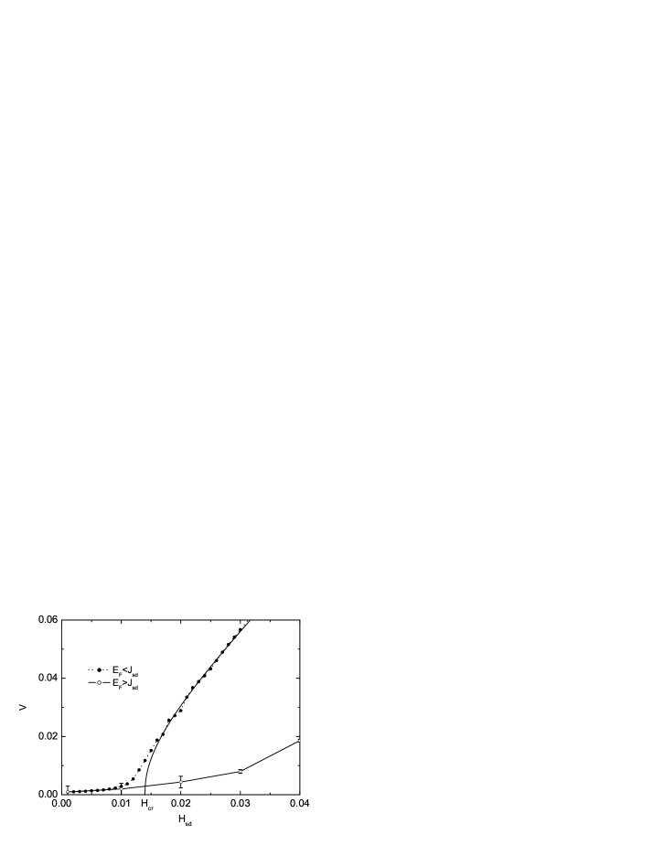
Figure 3: The domain wall velocity ($V$) as a function of the s-d exchange constant ($H_{\rm sd}$) that is related to the amplitude of the current. The initial velocity is plotted for the adiabatic case ($E_{\rm F}<J_{\rm sd}$, $E_{\rm F}=0.11$, $J_{\rm sd}=0.2$, bullets and dotted line) while the average velocity is shown for the mesoscopic case ($E_{\rm F}>J_{\rm sd}$, $E_{\rm F}=0.21$, $J_{\rm sd}=0.2$, circles). Error bars: square root of the variance of the velocity. Solid line: the analytical result $\propto\sqrt{H_{sd}^{2}-H_{\rm cr}^{2}}$, where $H_{\rm cr}$ is the critical s-d exchange constant that is estimated as $H_{\rm cr}\sim 0.014$.

In conclusion, we have numerically studied the dynamics of the domain wall driven by a mesoscopic current. We have treated the conduction electrons quantum mechanically. Spin-mixed states are taken into account. In the adiabatic case, $E_{\rm F}<J_{\rm sd}$, the contribution of the spin mixed state is equivalent to an additional external magnetic field which induces a residual velocity of the domain wall. In the mesoscopic region, $E_{\rm F}>J_{\rm sd}$, the spin precession of the conduction electrons induces spin wave excitations in the system of the local spins. We have pointed out that the presence of these spin waves enhances the displacement. The resulting average velocity of the domain wall is small compared with the one obtained from the adiabatic spin torque mechanism only. In the limit of small driving current the velocities of the adiabatic and the mesoscopic cases coincide within the error bars. Our results suggest that non-adiabatic effects, that can always be expected to be present in experiment, give rise to distortions of the local spin configuration and lead to a finite velocity of the wall even for currents below the critical value. We suggest that this is the microscopic mechanism that accounts for the non-adiabatic contribution towards the shape of the domain wall discussed earlier thiaville ; Li04b . This could explain very well the results of the recent experiments where rather small domain wall velocities have been found for currents that are an order of magnitude below the critical current Yamaguchi ; Tatara .

An alternative explanation of the experimentally observed velocities could be the presence of spin waves which could be due to temperature effects even for an adiabatic system. This would lead to much smaller velocities than predicted adiabatically (cf. Fig. 3). Furthermore, from our results, the spin-wave induced velocity is predicted to show large fluctuations that are consistent with the experimental observations Yamaguchi .

Finally, we want to point out that our calculations have been done for a general abstract model. By suitably adjusting the parameters, and by generalizing the model Hamiltonian, for instance by including more than one conduction channel, our method may be able to contribute to better understanding a variety of different experimental situations ranging from ferromagnetic nanowires to magnetic semiconductor nanostructures. In addition, since we treat the conduction electrons fully quantum mechanically, mesoscopic interference effects in the current as a function of time can in principle be expected — especially for magnetic semiconductor nanowires ohno ; ruester — that could be signaled in the dynamics of the domain wall. Whether or not this will be the case is an open question and the subject of future research.

- (1) L. Berger, Phys. Rev. B 33, 1572 (1986).
- (2) L. Berger, Phys. Rev. B 54, 9353 (1996).
- (3) J. C. Slonczewski, J. Magn. Magn. Mater. 159, L1 (1996).
- (4) Z. Li and S. Zhang, Phys. Rev. Lett. 92, 207203 (2004); Phys. Rev. B 70, 24417 (2004).
- (5) A. Thiaville, Y. Nakatami, J. Miltrat, Y. Suzuki, cond-mat/0407628 (2004).
- (6) S. Zhang and Z. Li, Phys. Rev. Lett. 93, 127204 (2004).
- (7) G. Tatara and H. Kohno, Phys. Rev. Lett. 92, 86601 (2004).
- (8) X. Waintal and M. Viret, Europhys. Lett. 65, 427 (2004).
- (9) S. E. Barnes and S. Maekawa, cond-mat/0410021 (2004).
- (10) A. Yamaguchi, T. Ono, S. Nasu, K. Miyake ,K. Mibu and T. Shinjo, Phys. Rev. Lett. 92, 77205 (2004).
- (11) M. Yamanouchi, D. Chiba, F. Matsukura and H. Ohno, Nature 428, 539 (2004).
- (12) E. Saitoh, H. Miyajima, T. Yamaoka and G. Tatara, Nature 432, 203 (2004).
- (13) J. B. Pendry, A. MacKinnon and P. J. Roberts, Proc. R. Soc. A 437, 67 (1992).
- (14) J. I. Ohe, M. Yamamoto and T. Ohtsuki, Phys. Rev. B 68, 165344 (2003).
- (15) J. I. Ohe and B. Kramer (to be published).
- (16) H. Ohno et al., Science 281, 951 (1998).
- (17) C. Ruester et al., Phys. Rev. Lett. 91, 216602 (2003).