Virtual-move Parallel Tempering

Abstract

We report a novel Monte Carlo scheme that greatly enhances the power of parallel-tempering simulations. In this method, we boost the accumulation of statistical averages by including information about all potential parallel tempering trial moves, rather than just those trial moves that are accepted. As a test, we compute the free-energy landscape for conformational changes in simple model proteins. With the new technique, the sampled region of the configurational space in which the free-energy landscape could be reliably estimated, increases by a factor 20.

The exponential increase in the speed of computers during the past decades has made it possible to perform simulations that were utterly unfeasible one generation ago. But in many cases, the development of more efficient algorithms has been at least as important.

One of the most widely used schemes to simulate many-body systems is the Markov-chain Monte Carlo method (MCMC) that was introduced in 1953 by Metropolis et al. Metropolis . In this algorithm the average properties of a system are estimated by performing a random walk in the configurational space, where each state is sampled with a frequency proportional to its Boltzmann weight. In the Metropolis algorithm, this is achieved by attempting random moves from the current state of the system to a new state. Depending on the ratio of the Boltzmann weights of the new and the old states, these trial moves may be either accepted or rejected. Metropolis et al. showed that the acceptance probability of trial moves can be chosen such that Boltzmann sampling is achieved.

One important application of the MC method is the estimation of the Landau free energy $F$ of the system as function of some order parameter

$$F\left(Q\right)=-kT\left[\ln P\left(Q\right)\right].$$

There are many situations where the MCMC method does not yield an accurate estimate of $F$, because it fails to explore configuration space efficiently. This is, for instance, the case in “glassy” systems that tend to get trapped for long times in small pockets of configuration space. In the early 1990’s the so-called parallel-tempering (PT) technique was introduced to speed up the sampling in such systems Parallel Tempering ; Parallel Tempering 2 ; Parallel Tempering 3 .

In a parallel-tempering Monte Carlo simulation, $n$ simulations of a particular model system are carried out in parallel at different temperatures (or other at different values of some other thermodynamic field, such as the chemical potential or a biasing potential). Each of these copies of the system is called replica. In addition to the regular MC trial moves, one occasionally attempts to swap the temperatures of a pair of these systems (say $i$ and $j$). The swapping move between temperature $i$ and $j$, is accepted or rejected according to a criterion that guarantees detailed balance, e.g.:

$$P_{acc}(ij)=\frac{e^{\Delta\beta_{ij}\Delta E_{ij}}}{1+e^{\Delta\beta_{ij}\Delta E_{ij}}}$$ (1)

where $\Delta\beta_{ij}$ is the difference of the inverse of swapping temperatures, and $\Delta E_{ij}$ is the energy difference of the two configurations. Although there are other valid acceptance rules, we used the one in Eq.1 because it was easy to implement.

To facilitate the sampling of high free-energy states,”difficult” regions, we use the Adaptive Umbrella Sampling umbrella ; umbrella 2 . In this (iterative) scheme, a biasing potential is constructed using the histogram of the states, sampled during an iteration as follows

$$W_{I}\left(Q,T\right)=W_{I-1}\left(Q,T\right)-a\ln\left(P_{I}\left(Q\right)\right),$$ (2)

where $W$ is the biasing potential function of an order parameter $Q$, $I$ is the iteration number, $a$ is a constant that controls the rate of convergence of $W$ (a typical value for $a$ is $0.05$), and $T$ is the temperature. After iteration, $W$ converges to the Landau free energy. As a consequence, $P(Q)\sim\exp(-\beta F(q))\exp(W(Q))$ becomes essentially flat and the biased sampling explores a larger fraction of the configuration space. During the MC sampling, we include the bias, and only at the end of the simulation we compute the free energy $F\left(Q\right)$ from

$$F\left(Q\right)=-kT\left[\ln P\left(Q\right)+W\left(Q,T\right)\right],$$

where $P\left(Q\right)$ is the probability of observing a state characterized by the order parameter $Q$, and $W\left(Q,T\right)$ is the biasing potential of the last iteration computed at temperature $T$. Combined with Parallel Tempering, the acceptance rule for the temperature swapping move is then

$$acc_{ij} = \frac{e^{\Delta\beta_{ij}\Delta E_{ij}+\Delta W_{ij}}}{1+e^{\Delta\beta_{ij}\Delta E_{ij}+\Delta W_{ij}}}$$ (3)

$$\Delta W_{ij} = W_{I}(Q_{i},T_{j})-W_{I}(Q_{j},T_{j})+$$ (4)

$$W_{I}(Q_{j},T_{i})-W_{I}(Q_{i},T_{i})$$

where $i$ and $j$ are replica indices, and $I$ is the iteration number. We refer to this scheme as APT (Adaptive Parallel Tempering) The Paper ; Multicanonical Parallel Tempering .

In the conventional MCMC method all information about rejected trial moves is discarded. Recently one of us has proposed a scheme that makes it possible to include the contributions of rejected configurations in the sampling of averages WasteR . In the present paper, we show how this approach can be used to increase the power of the parallel-tempering scheme.

In this scheme, we only retain information about PT moves that have been accepted. However, in the spirit of refs. WasteR , we can include the contribution of all PT trial moves, irrespective of whether they are accepted. The weight of the contribution of such a virtual move is directly related to its acceptance probability. For instance, if we use the symmetric acceptance rule for MC trial moves, then the weights of the original and new (trial) state in the sampling of virtual moves are given by

$$P_{N} = \frac{e^{\Delta\beta\Delta E_{O\rightarrow N}+\Delta W_{O\rightarrow N}}}{1+e^{\Delta\beta\Delta E_{O\rightarrow N}+\Delta W_{O\rightarrow N}}}$$

$$P_{O} = \frac{1}{1+e^{\Delta\beta\Delta E_{O\rightarrow N}+\Delta W_{O\rightarrow N}}}\,,$$

where $\Delta W_{O\rightarrow N}$ is defined in Eq.4. We are not limited to a single trial swap of state $i$ with a given state $j$. Rather, we can include all possible trial swaps between the temperature state $i$ and all $N-1$ remaining temperatures. Our estimate for the contribution to the probability distribution $P_{i}$ corresponding to temperature $i$ is then given by the following sum

$$P_{i}\left(Q\right) = \sum_{j=1}^{N-1}\left(\frac{1}{1+e^{\Delta\beta_{ij}\Delta E_{ij}+\Delta W_{ij}}}\right)\delta\left(Q_{i}-Q\right)+$$

$$\sum_{j=1}^{N-1}\left(\frac{e^{\Delta\beta_{ij}\Delta E_{ij}+\Delta W_{ij}}}{1+e^{\Delta\beta_{ij}\Delta E_{ij}+\Delta W_{ij}}}\right)\delta\left(Q_{j}-Q\right),$$

where the delta functions select the configurations with order parameter $Q$. As we now combine the Parallel tempering algorithm with a set of parallel virtual moves, we refer to the present scheme as Virtual-move Parallel Tempering (VMPT).

To measure the efficiency of VMPT, we computed the free energy landscape of a simple lattice-protein model. In this model, interaction with a substrate can induce a conformational change in the proteins. For the same system we had already explored the use of the conventional adaptive PT scheme The Paper .

Specifically, the model protein that we consider represents a heteropolymer containing 80 amino acids, while the substrate has a fixed space arrangement and contains 40 residues, see Fig.1. The configurational energy of the system is defined as

$$E_{C}=E_{\textrm{intra}}+E_{\textrm{inter}}=\sum_{i}^{N_{C}}\left[\sum_{j\neq i}^{N_{C}}C_{ij}S_{ij}+\sum_{j^{\prime}\neq i}^{N_{S}}C_{ij^{\prime}}S_{ij^{\prime}}\right],$$ (5)

where the indices $i$ and $j$ run over the residues of the protein, while $j^{\prime}$ runs only over the elements of the substrate, $C$ is the contact defined as

$$C_{ij}=\left\{\begin{array}[]{cc}1&\textrm{if i neighbor of j}\\ 0&\textrm{otherwise}\,.\end{array}\right.$$ (6)

and $S_{ij}$ is the interaction matrix. For $S$ we use the 20 by 20 matrix fitted by Miyazawa and Jernigan S.Miyazawa on the basis of the frequency of contacts between each pair of amino acids in nature.

We change the identity of the amino acids along the chain by “point mutations” which, in this context, means: changes of a single amino acid. In doing so we explore the sequence space of the protein and the substrate, and we minimize at the same time the configurational energy of the system in two distinct configurations, one bound (Fig.1.a) and one unbound (Fig.1.b). The design scheme is the same as used in Ref.The Paper . In this scheme, trial mutations are accepted if the Monte Carlo acceptance criterion is satisfied for both configurations.

The result of the design process is a model protein that has the ability to change its conformation when bound to the substrate. The sampling of the configurations is performed with three basic moves: corner-flip, crankshaft, branch rotation. The corner-flip involves a rotation of 180 degrees of a given particle around the line joining its neighbors along the chain. The crankshaft move is a rotation by 90 degrees of two consecutive particles. A branch rotation is a turn, around a randomly chosen pivot particle, of the whole section starting from the pivot particle and going to the end of the chain. For all these moves we use a symmetric acceptance rule with the addition of the biasing potential calculated with the umbrella sampling scheme (Eq.2)

$$acc_{O\rightarrow N}=\frac{e^{\beta\Delta E_{O\rightarrow N}+\Delta W_{O\rightarrow N}}}{1+e^{\beta\Delta E_{O\rightarrow N}+\Delta W_{O\rightarrow N}}},$$ (7)

where $\Delta E_{O\rightarrow N}$ is the energy difference between the new and the old state (Eq.5), and $\Delta W_{O\rightarrow N}$ is the difference in the bias potential from the same states (Eq.2). We sample the free energy, as a function of two order parameters, of which the first is the conformational energy defined in Eq.5, and the second is the difference of the number of contacts belonging to two reference structures (e.g. 1 and 2) i.e.

$$Q(C)=\sum_{i<j}^{N}\left[C_{ij}^{\left(1\right)}C_{ij}-C_{ij}^{\left(2\right)}C_{ij}\right]\,,$$ (8)

where $C_{ij}^{\left(1\right)}$ and $C_{ij}^{\left(2\right)}$ are the contact maps of the reference structures, and $C_{ij}$ is the contact map of the instantaneous configuration. The order parameter that measures the change in the number of native contacts is defined as follows: as we consider two distinct native states, we take these as the reference structures. Every contact that occurs to state 1 has a value and every contact that belongs to structure 2 has a value $-1$. Contacts that appear in both $1$ and $2$, or do not appear in neither of the two, do not contribute to the order parameter.

The reason why we assign negative values to native contacts of structure 2, is that we compute the free energy difference between the protein in configuration 1 and 2. If we would have assigned 0 to the contacts of structure 2 then we would not have been able to distinguish it from unfolded configurations that do no have any native contacts at all. For our specific case, $C_{ij}^{\left(1\right)}$ represents the structure in Fig.1.a, while $C_{ij}^{\left(2\right)}$corresponds to the one shown in Fig.1.b, and $Q$ has values between -15 and 30. Because the number of native contacts includes the contacts with the substrate of the reference state, it can be used to compute the free energy difference between the unbound state and the specifically bound one.

We performed 15 simulations, 5 of them with VMPT (using the parameters in Tab.1.I) and the other 10 with APT ( 5 using the parameters in Tab.1.I, and 5 with the parameters in Tab.1.II). In Fig.2 we compare the average free energies at $T=0.1$ (with error bars). In this figure, we only show those free energies that were sampled in all the 5 simulations of each group. From the figure it is clear that the VMPT approach leads to a much better sampling of the free-energy landscape. The advantage of the VMPT approach becomes even more obvious if we plot the free energy “landscape” as function of two order parameters (viz. the conformational energy (Eq.5) and the number of native contacts). In this case the APT method is almost useless as only small fragments of the free-energy landscape can be reconstructed. The total number of points sampled with VMPT is 20 times larger than with APT, and the energy range that is probed, is one order of magnitude larger (see Fig.3).

To check the accuracy of the VMPT method, we compared the average free energy obtained by APT and VMPT at high temperatures where the APT scheme works reasonably well. As can be seen in Fig.4 the two methods agree well in this regime (be it that a much longer APT simulation was needed). Even though the APT runs required 20 times more MC cycles, it still probes about 30% less of the free-energy landscape than the VMPT scheme.

As the implementation described above is not based on a particular feature of the system under study, the results obtained in this study suggest that the VMPT method may be useful for the study of any system that is normally simulated using Parallel Tempering. Examples of the application of Parallel Tempering in fully atomistic simulations of protein folding can be found in refs. Applica1 ; Applica2 .

Simulation	Temperatures	Number of Iterations	Sampling Steps	APT exec time (sec)	VMPT exec Time (sec)
I	0.1 0.125 0.143 0.167 0.2 0.222 0.23 0.25 0.270000 0.29 0.31 0.33 0.350000 0.37 0.4 0.444 0.5	400	$4\,10^{8}$	2600	3200
II	0.1 0.125 0.143 0.167 0.2 0.222 0.23 0.25 0.270000 0.29 0.31 0.33 0.350000 0.37 0.4 0.444 0.5	1000	$2\,10^{10}$	150000

Table 1: Simulation parameters used for comparing the VMPT algorithm with the old scheme. In Simul. I we used the same parameters for both algorithms. The results in Fig.2 show that VMPT was much more efficient in sampling the free energy . In Simul .II, we increased by two orders of magnitude the number of steps of the simulation with APT to obtain a sampling of $F\left(Q\right)$comparable to the one computed using the new VMPT scheme (Fig.4). Execution times computed on a SGI Altix 3700 with Intel Itanium II, 1,3 GHz

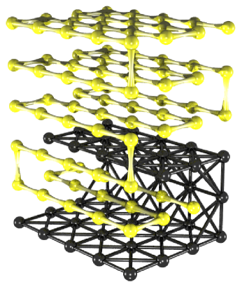
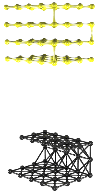
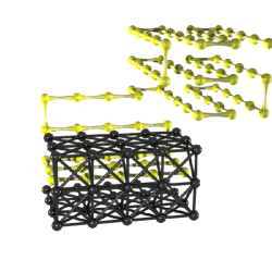
Figure 1: (Color online) Spatial arrangement of the chain in the structures used to test the model (a , b) , and intermediate structure ($Q=25$).

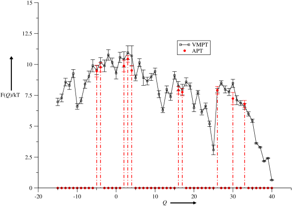
Figure 2: (Color online) Average free energy computed with 5 run (10^8 MC steps Tab.1.I) of the old scheme, compared with the result of 5 VMPT simulation ( 10^8 MC steps Tab.1.I), at $T=0.1$. The points with $F=0$ correspond to values of $Q$ that have not been sampled.

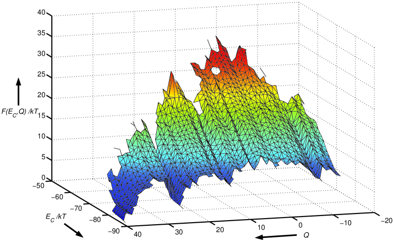
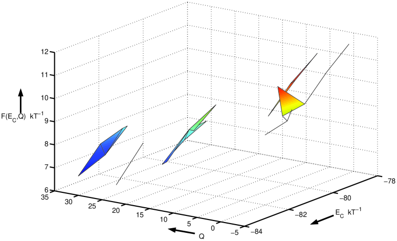
Figure 3: (Color online) Plot of the free energy landscapes computed with the algorithm VMPT (a) and the standard scheme APT (b). The free energies $F(E_{C},Q)$ are function of the conformational energy $E_{C}$ (Eq.5) and of the number of native contacts $Q$ (Eq.8). It is important to notice the big difference in the sampling, in fact the number of points sampled with VMPT is 30 times bigger than the one obtained with APT.

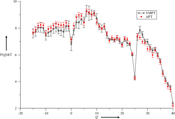
Figure 4: (Color online) Average free energy computed with 5 long run (10^10 MC steps Tab.1.II) of the old scheme, compared with the result of 5 shorter VMPT simulation ( 10^8 MC steps Tab.1.I), at $T=0.5$

References

- (1) N. Metropolis, A. W. Rosenbluth, M. N. Rosenbluth, A. N. Teller, and E. Teller, J. Chem. Phys. 21, 1087 (1953)
- (2) D. Frenkel, PNAS. 101, 17571 (2004).
- (3) D. Frenkel and B. Smit, Understanding Molecular Simulations, 389 (Accademic Press 2002)
- (4) A.P. Lyubartsev, A.A. Martsinovski, S.V. Shevkunov, and P.N. Vorontsov-Vel’yaminov, J. Chem. Phys. 96, 1776 (1992)
- (5) E. Marinari and G. Parisi, Europhys. Lett. 19, 451 (1992)
- (6) C.J. Geyer and E.A. Thompson, J. Am. Stat. Soc. 90, 909 (1995)
- (7) S. Miyazawa and R.Jernigan, Macromolecules 18, 534 (1985), table VI
- (8) G.M. Torrie and J.P. Valleau, J. Comp. Phys., 23, 187(1977)
- (9) B.A. Berg and T. Neuhaus, Phys. Rev. Lett. 68, 9 (1992)
- (10) I. Coluzza,H.G. Muller, and D. Frenkel, Phys Rev E, 68 (046703), (2003)
- (11) R. Faller, Q. Yan, and J.J. de Pablo, J. Chem. Phys. 13, 5419 (2002)
- (12) Lin C.Y., Hu C.K,. and Hansmann U.H.E., Proteins-Str. Fun. and Gen. 52, 436 (2003)
- (13) Schug A., Wenzel W., Europhys. Lett. 67, 307 (2004)