Reaction-diffusion processes on correlated and uncorrelated scale-free networks

Abstract

We compare reaction-diffusion processes of the $A+A\to 0$ type on scale-free networks created with either the configuration model or the uncorrelated configuration model. We show via simulations that except for the difference in the behavior of the two models, different results are observed within the same model when the minimum number of connections for a node varies from $k_{\rm min}=1$ to $k_{\rm min}=2$. This difference is attributed to the varying local properties of the two systems. In all cases we are able to identify a power law behavior of the density decay with time with an exponent $f>1$, considerably larger than its lattice counterpart.

Recently, a growing interest for dynamic processes taking place on scale-free networks has arisen AB ; DM . A scale-free network is one where the node connectivity $k$ (number of links on a node) follows a power-law distribution of the form

$$P(k)\sim k^{-\gamma}\,,$$ (1)

where $\gamma$ is a positive number, typically in the range $2<\gamma<4$. In this frame, we recently presented GA simulation results for reaction-diffusion processes both of the type $A+A\to 0$ and $A+B\to 0$, where the substrate for diffusion is a scale-free network. Following this, Catanzaro et al. CBPSa developed an elegant theory for the $A+A\to 0$ process, which applies on networks created with the uncorrelated configuration model (UCM) CBPSb . Their analytic results were found to be in good agreement to their simulations, but were deviating from the results in Ref. GA , where the networks were created with the configuration model (CM). The authors attributed the difference of the results on the different method of preparing the networks. In this Brief Report we directly compare results for both the UCM and CM models.

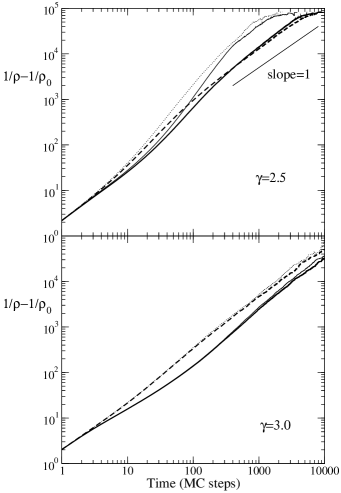
Figure 1: Plot of the reaction progress $1/\rho-1/\rho_{0}$, as a function of time for the A+A$\to$0 reaction on scale-free networks of (a) $\gamma=2.5$, and (b) $\gamma=3.0$. Results correspond to CM (thin lines) and UCM (thick lines) models, with $k_{\rm min}=1$ (solid lines) and $k_{\rm min}=2$ (dashed lines). The initial density was $\rho_{0}=0.5$. All results correspond to networks of $N=10^{6}$ nodes.

The Configuration Model (CM) has become more or less the standard for simulating networks of a given $\gamma$ value in the literature. For each one of the $N$ system nodes a random $k$ value is assigned, drawn from the probability distribution function of Eq. (1). Pairs of links are then randomly chosen between the nodes, taking care that no double links between two nodes or self-links in the same node are established. When the maximum value of $k$ is not pre-defined, then the natural upper cutoff scales with the system size as $k_{\rm max}\sim N^{1/(\gamma-1)}$. This model is known to create correlations in the connectivity distribution between the system nodes for $\gamma<3$, in the sense that the average connectivity of a node’s neighbors depends on its rank $k$. In other words, nodes that are highly connected prefer to attach to nodes with lower $k$-values, rather than to equally well-connected nodes. The Uncorrelated Configuration Model (UCM) uses the same construction algorithm, with the difference that the upper cutoff is fixed in advance to $k_{\rm max}=N^{1/2}$. Then, it has been shown CBPSb that connectivity correlations dissapear and the average connectivity for the neighbors of any node is constant.

In Ref. GA we had found that the reaction rate was evolving surprisingly faster than on regular lattices. The variation of the particle concentration $\rho(t)$ was still following a power law with time $t$ of the form

$$\frac{1}{\rho(t)}-\frac{1}{\rho_{0}}\sim t^{f}\,,$$ (2)

but with a value $f>1$ for $\gamma<3.5$. This result was valid asymptotically within the simulation accuracy, and before finite-size effects settled in. The networks that we had used had been created with the CM model with a minimum value for the connectivity of a node (lower cutoff) $k_{\rm min}=1$. Since this process may create isolated clusters, we only had used the largest cluster which, depending on the value of $\gamma$, would span from 35% to 100% of the system nodes.

In Ref. CBPSa the $A+A\to 0$ process was studied, and it was analytically found that for an infinite size network the exponent $f$ of Eq. (2) is given by $f=1/(\gamma-2)$ when $2<\gamma<3$, i.e. again $f>1$. For $\gamma=3.0$ the behavior was predicted analytically to be $1/\rho\sim t\ln{t}$. However, for finite size networks and long times the behavior of $1/\rho$ is masked for all $\gamma$ by the mean-field exponent $f=1$, which seems to also be valid asymptotically from the simulation results. Both the analytic solution and the simulations in that paper were based on networks created under the UCM model, with a lower cutoff value of $k_{\rm min}=2$. The authors of Ref. CBPSa reported that in their simulations it was not possible to find a noticeable regime with $f>1$, and they attribute the discrepancy between the two studies solely in the different network creation method. We here argue that a power law regime with $f>1$ is indeed present and clearly identified in all cases. Additionally, a very important factor is the lower cutoff value, $k_{\rm min}$.

In the present Report we present and compare simulation results for both the CM and UCM models with $k_{\rm min}=1$ and $k_{\rm min}=2$. Results for the time evolution of the particle density in all four possible cases are shown in Fig. 1. All four curves in the case of $\gamma=2.5$ (Fig. 1a) behave differently from each other. The CM and UCM models clearly yield different results, but even within UCM or CM the curves for $k_{\rm min}=1$ and $k_{\rm min}=2$ deviate from each other. The main difference is that the crossover to the power law behavior for $k_{\rm min}=1$ appears later in time, and the asymptotic mean-field behavior ($f=1$) also exhibits itself roughly one decade later.

The case of $\gamma=3.0$ (Fig. 1b) is simpler. For this $\gamma$ value the two models (CM and UCM) are expected to coincide, since in general the natural upper cutoff in the CM model scales as $k_{c}\sim N^{1/\gamma-1}$, and for $\gamma=3.0$ the value $k_{c}=N^{1/2}$ is exactly the same as in the UCM model. This coincidence is shown to be valid in the figure. However, the results for $k_{\rm min}=1$ are still different than the results for $k_{\rm min}=2$. The crossover to the power-law behavior is not as prominent as in the case of $k_{\rm min}=1$.

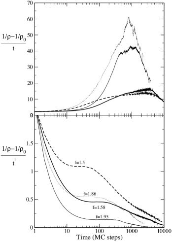
Figure 2: Results for networks with $\gamma=2.5$. Plots of inverse particles density ($1/\rho-1/\rho_{0}$) divided by (a) $t$ and (b) $t^{f}$, as a function of time. Thick lines correspond to the UCM and thin lines to the CM model while in solid curves $k_{\rm min}=1$ and in dashed lines $k_{\rm min}=2$. In (b) the $f$ values are shown on the plot.

We then assess whether there exists an observable power-law behavior in these curves and whether asymptotically a linear regime masks this power-law. The results for $\gamma=2.5$ are presented in Fig. 2. In the first plot we divide the curves of Fig. 1a by the linear function $t$. If asymptotically the expected behavior is linear ($f=1$ in Eq. 2) then we expect that this division will yield a constant value, i.e. a horizontal line parallel to the x-axis. The only case which is close to this behavior is that of the UCM model and $k_{\rm min}=2$ (thick dashed line in the plot). Even then, the result is not entirely satisfactory, and the curve seems to have a slope greater than 0. Notice also that although from Fig. 1a one can visually get the impression that a slope of 1 is describing quite accurately this curve, the more detailed analysis in Fig. 2a reveals that this is not true. In all other cases, there are only weak hints for a parallel line, but it cannot be argued that this linear relation is in general valid, and this is why it was not observed in Ref. GA . The abruptly falling curves at longer times are due to very low particle densities, where less than 10 particles remain in the system.

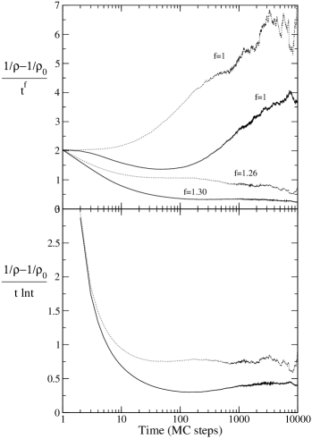
Figure 3: Results for networks with $\gamma=3.0$. Plots of inverse particle density ($1/\rho-1/\rho_{0}$) divided by (a) $t^{f}$ and (b) $t\ln{t}$, as a function of time. The CM and UCM models yield the same curves, so we only present results for CM with $k_{\rm min}=1$ (solid lines) and $k_{\rm min}=2$ (dashed lines).

In Fig. 2b, we also test the hypothesis for power-law behavior by dividing the raw data of Fig. 1a by $t^{f}$. Since curves corresponding to different models exhibit varying exponents $f$ we choose the value of $f$ that maximizes the extent of the horizontal part in each line.

The presence of a power law regime is clear in all occasions, but it is also noteworthy that the validity of the power law lies in a narrower time range for $k_{\rm min}=2$, and especially from the UCM model, rendering this estimation more difficult. Most probably, this is the reason that the authors of Ref. CBPSa did not characterize this regime. The case where in a simulation a particular power law shows only in a very limited time domain is not unusual, see e.g. the Zeldovich behavior of the $A+B$ reaction on a 3-dimensional lattice, where the density exponent has a nominal value of $f=0.75$, which shows only in one time decade Argyrakis . The slopes of the curves for $k_{\rm min}=1$ are consistently larger compared to the slopes of the $k_{\rm min}=2$ curves. We also note that the analytical prediction of Ref. CBPSa predicts a slope of $f=2.0$, which is very close to the slope of the CM model for $k_{\rm min}=1$, but deviates remarkably from the slope of the UCM model, although this prediction was based on the uncorrelated network hypothesis.

We have already seen that when $\gamma=3.0$ the CM and UCM models are identical. For clarity in Fig. 3 we analyze only the results of CM. Again, the hypothesis that asymptotically there is a linear increase is not directly supported from our simulation results. On the contrary, if we consider a power law fit for the intermediate time regime, we observe an extended horizontal part that spans a few decades. The slope for both $k_{\rm min}=1$ and 2 are similar and close to $1.3$. An increase in the network size $N$ has been shown to further extend the region of validity for the power-law behavior in the $f>1$ regime (see e.g. Fig. 1 of GA and Fig. 6 of CBPSa ).

The analytic considerations in Ref. CBPSa for $\gamma=3.0$ predict a logarithmic correction ($1/\rho\sim t\ln{t}$). In general, it is not easy to distinguish between this form and a power law curve. However, when we divide our raw simulation data with the $t\ln{t}$ function in Fig. 3b, we observe that for $k_{\rm min}=2$ there is an excellent agreement, but this function fails to reliably describe the results for $k_{\rm min}=1$.

The most probable explanation for the difference in the results for the varying $k_{\rm min}$ values is that the local environment in the case of $k_{\rm min}=1$ is remarkably different than when $k_{\rm min}=2$. Although $k_{\rm min}=2$ is known to yield one giant connected cluster Cohen , its structural characteristics seem to be modified, basically because of the tree-like features (many nodes are connected to just one neighbor). Bottlenecks and revisitations are, thus, more frequent than in the case where a larger lower cutoff is used.

In short, the value of the exponent characterizing a reaction-diffusion process on scale-free networks depends not only on the network construction model, but is also sensitive to the lower cutoff value for the connectivity $k_{\rm min}$, although such a dependence has not been predicted analytically. More importantly, we have verified the existence of a power law regime that is large enough to be observable in all cases, while a careful analysis also revealed that an asymptotic linear behavior is not in general valid.

References

- (1) R. Albert and A.-L. Barabasi, Rev. Mod. Phys. 74, 47 (2002).
- (2) S.N. Dorogovtsev and J.F.F. Mendes, Adv. Phys. 51, 1079 (2002).
- (3) L.K. Gallos and P. Argyrakis, Phys. Rev. Lett. 92, 138301 (2004).
- (4) M. Catanzaro, M. Boguñá and R. Pastor-Satorras, e-print cond-mat/0407447 (2004).
- (5) M. Catanzaro, M. Boguñá and R. Pastor-Satorras, e-print cond-mat/0408110 (2004).
- (6) P. Argyrakis and R. Kopelman, Phys. Rev. A 45, 5814 (1992).
- (7) R. Cohen, K. Erez, D. ben Avraham, and S. Havlin, Phys. Rev. Lett. 85, 4626 (2000).