Tunable Fano effect in parallel-coupled double quantum dot system

Abstract

With the help of the Green function technique and the equation of motion approach, the electronic transport through a parallel-coupled double quantum dot(DQD) is theoretically studied. Owing to the inter-dot coupling, the bonding and antibonding states of the artificial quantum-dot-molecule may constitute an appropriate basis set. Based on this picture, the Fano interference in the conductance spectra of the DQD system is readily explained. The possibility of manipulating the Fano lineshape in the tunneling spectra of the DQD system is explored by tuning the dot-lead coupling, the inter-dot coupling, the magnetic flux threading the ring connecting dots and leads, and the flux difference between two sub-rings. It has been found that by making use of various tuning, the direction of the asymmetric tail of Fano lineshape may be flipped by external fields, and the continuous conductance spectra may be magnetically manipulated with lineshape retained. More importantly, by adjusting the magnetic flux, the function of two molecular states can be exchanged, giving rise to a swap effect, which might play a role as a qubit in the quantum computation.

I Introduction

When the phase coherence of electrons passing through a mesoscopic system is retained, a number of quantum interference phenomena will occur. Recent advances in nano-technologies have attracted much attention to the quantum coherence phenomena in the resonant tunneling processes of the quantum dot(QD) systems,nato in which the typical length scale can be shorter than or comparable to the mean free path of electrons and the wave nature of electrons plays a decisive role. In the past decade, the widely adopted method of studying the phase coherence of a traversing electron through a QD is to measure the magnetic-flux-dependent current through an Aharonov-Bohm(AB) interferometer by inserting the QD into one of its arms.ab The observed magnetic-oscillation of the current will be the indication of the coherent transport through the QD, provided that at least partial coherence of electrons is kept. Holleitner2001 ; Holleitner2002 ; Holleitner2003 ; Blick2003 ; yacoby ; schuster ; buks ; wiel ; yji ; Kobayashi2002 ; Kobayashi2003

Fano resonances is another good probe for the phase coherence in the QD system.Kobayashi2002 ; Kobayashi2003 ; gores ; zacharia ; johnson It is known that the Fano resonance stems from quantum interference between resonant and nonresonant processes,fano and manifests itself in spectra as asymmetric lineshape in a large variety of experiments. Unlike the conventional Fano resonance,conventional1 ; conventional2 ; conventional3 ; conventional4 the Fano effect in QD system has its advantage in that its key parameters can be readily tuned. Suppose that a discrete level inside the QD acts as a Breit-Wigner-type scatter and is broadened by a factor of $\Gamma$ due to couplings with the continua in leads. The key to realize the Fano effect in the conductance spectra is that, within $\Gamma$ the phase of the electron should smoothly change by $\pi$ on the resonance.schuster The first observation of the Fano lineshape in the QD system was reported by Göres et al.gores ; zacharia in the single-electron-transistor experiments. Recently, K. Kobayashi et al. carried out research on magnetically and electrostatically tunable Fano effect in a QD embedded in an AB ring,Kobayashi2002 ; Kobayashi2003 and A.C. Johnson et al. investigated a tunable Fano interferometer consisting of a QD coupled to a one-dimensional channel via tunneling and observed the Coulomb-modified Fano resonances.johnson

The double quantum dot(DQD) system, including the series-coupled DQDWaugh1995 ; Blick1998 ; Oosterkamp1998 ; Qin2001 and parallel-coupled DQD,Holleitner2001 ; Holleitner2002 ; Holleitner2003 ; Blick2003 ; jcchen makes the quantum transport phenomena rich and varied. The parallel-coupled DQD system is of particular interest, in which two QD’s are respectively embedded into opposite arms of the AB ring, coupled each other via barrier tunneling, and coupled to two leads roughly equally. As a controllable two-level system, it is appealing for the parallel-coupled DQD system to become one of promising candidates for the quantum bit in quantum computation based on solid state devices.loss ; hu The entangled quantum states required for performing the quantum computation demand a high degree of phase coherence in the system.highcoherence Being a probe of phase coherence,clerk if the Fano effect in the parallel-coupled DQD system is tunable and exhibits the swap effect, it is certainly of practical importance.

Inspired by recent experimental advances in the parallel DQD,Holleitner2001 ; Holleitner2002 ; Holleitner2003 ; Blick2003 ; jcchen several groups have attempted to address this multi-path system theoretically, and predicted the Fano resonance in the parallel-coupled DQD system.mahan ; kang ; guevara ; baizhiming ; bingdong ; guevara2 However, it seems that a physically transparent picture for the Fano effect in the DQD system is still lacking. For example, it is unclear what the resonant and nonresonant channels are in this Fano system. Moreover, a systematic study is required for exploring various possibilities of tuning Fano effect with external fields. In this paper, we intend to provide with a natural yet simple explanation for the Fano effect in the parallel-coupled DQD, and propose several ways to control the Fano resonance in the conductance spectra by the electrostatic and magnetic approaches.

The paper is organized as follows. In Sec.II, a widely used two-level Fano-Anderson model is introduced with an inter-dot coupling term added. Since the coupled quantum dots may be considered as an artificial QD-molecules,livermore an effective Hamiltonian in terms of the bonding and antibonding states of the QD-molecule may form an appropriate working basis. Thus with the help of the Green function technique and the equation of motion method,haug the density of states is calculated in three asymmetric configurations classified according to the spatial symmetry of the dot-lead coupling.konig In Sec. III, the conductance formula is derived for this system,datta ; meir whereby the Fano lineshape in conductance spectra is calculated in the absence of the magnetic flux. In Sec.IV, a simple mechanism explaining the Fano lineshape in the DQD conductance spectrum is presented. Then, the possibilities of tuning the conductance lineshape by various electrostatic and magnetic methods are described in details, and several novel effects are predicted. Most importantly, by tuning the the total magnetic flux, or the flux difference between the left and right parts of the AB ring, the swap effect between two resonance peaks in the conductance spectra is predicted, which might be of potential application as a type of C-Not gate in the quantum computation. Finally, a brief summary is drawn and presented.

II Physical Model

We start with the Fano-Anderson model for the parallel-coupled DQD where the discrete states in two quantum dots are coupled each other via tunneling. (Fig.1a) Then the Hamiltonian reads

$$H=H_{leads}+H_{DD}+H_{T}.$$ (1)

The $H_{leads}$ in Eq.(1) represents the noninteracting electron gas in the left(L) and right(R) leads,

$$H_{leads}=\sum_{k,\alpha=L,R}\varepsilon_{k\alpha}c_{k\alpha}^{\dagger}c_{k\alpha},$$ (2)

where, $c_{k\alpha}^{\dagger},c_{k\alpha}$ are the creation and annihilation operators for a continuum in the lead $\alpha$ with energy $\varepsilon_{k\alpha}$. The $H_{DD}$ in Eq.(1) describes the QD electrons and their mutual coupling in the DQD, i.e.

$$H_{DD}=\sum_{i=1,2}\varepsilon_{i}d_{i}^{\dagger}d_{i}-t_{c}e^{i\theta}d_{1}^{\dagger}d_{2}-t_{c}e^{-i\theta}d_{2}^{\dagger}d_{1}.$$ (3)

The first term in Eq.(3), $d_{i}^{\dagger}$ $(d_{i})$, represents the create (annihilate) operator of the electron with the energy $\varepsilon_{i}$ in the dot $i$. The second and third terms in Eq.(3) denote the inter-dot coupling, in which $t_{c}$ is the coupling strength taken as a real parameter, and $\theta$ denotes a phase shift related to the flux difference between the left and right sub-rings. The $H_{T}$ in Eq.(1) represents the tunneling coupling between the QD and lead electrons,

$$H_{T}= \sum_{k,{\alpha}=L,R}\sum_{i=1,2}V_{\alpha i}d_{i}^{\dagger}c_{k{\alpha}}+h.c.,$$ (4)

where the tunneling matrix element $V_{L1}=|V_{L1}|e^{i\frac{\phi}{4}},V_{L2}^{*}=|V_{L2}|e^{i\frac{\phi}{4}},V_{R1}^{*}=|V_{R1}|e^{i\frac{\phi}{4}}$, and $V_{R2}=|V_{R2}|e^{i\frac{\phi}{4}}$. Here for the sake of simplicity, $V_{\alpha i}$ is assumed to be independent of $k$, and the phase shift due to the total magnetic flux threading into the AB ring, $\phi$, is assumed to distribute evenly among 4 sections of the DQD-AB ring. Namely, $\phi=2\pi(\Phi_{R}+\Phi_{L})/\Phi_{0}$, where the flux quantum $\Phi_{0}=hc/e$. Thus, $\theta=\pi(\Phi_{R}-\Phi_{L})/\Phi_{0}$. In the following calculation, we define the line-width matrix as $\Gamma^{\alpha}_{ij}=\sum_{k}V_{\alpha i}V^{*}_{\alpha j}2\pi\delta(\varepsilon-\varepsilon_{k{\alpha}})$ (${\alpha}=L,R)$ and $\mathbf{\Gamma}=\mathbf{\Gamma}^{L}+\mathbf{\Gamma}^{R}$. According to Fig.1(a), the line-width matrices in the QD representation read

$$\mathbf{\Gamma}^{L}=\left(\begin{array}[]{cc}\Gamma^{L}_{1}&\sqrt{\Gamma^{L}_{1}\Gamma^{L}_{2}}e^{i\frac{\phi}{2}}\\ \sqrt{\Gamma^{L}_{1}\Gamma^{L}_{2}}e^{-i\frac{\phi}{2}}&\Gamma^{L}_{2}\end{array}\right),$$

and

$$\mathbf{\Gamma}^{R}=\left(\begin{array}[]{cc}\Gamma^{R}_{1}&\sqrt{\Gamma^{R}_{1}\Gamma^{R}_{2}}e^{-i\frac{\phi}{2}}\\ \sqrt{\Gamma^{R}_{1}\Gamma^{R}_{2}}e^{i\frac{\phi}{2}}&\Gamma^{R}_{2}\end{array}\right),$$ (5)

where $\Gamma^{\alpha}_{i}$ is short for $\Gamma^{\alpha}_{ii}$ .

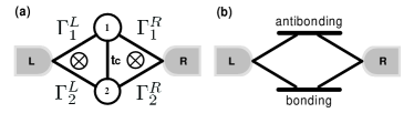
Figure 1: (a) Schematic diagram for a tunneling-coupled parallel DQD system. (b) Schematic diagram of the parallel-coupled DQD system in the molecular orbital representation.

To make the physical picture clearer and formalism simpler, it is attractive to introduce a QD-molecule representation by transforming two tunneling-coupled QD levels into the bonding and antibonding states of the QD-molecule. The operator for a molecule state can be expressed as a linear superposition of the QD operators as

$$\left(\begin{array}[]{c}f_{+}\\ f_{-}\end{array}\right)=\left(\begin{array}[]{cc}\cos\beta e^{-i\theta}&-\sin\beta\\ \sin\beta&\cos\beta e^{i\theta}\end{array}\right)\left(\begin{array}[]{c}d_{1}\\ d_{2}\end{array}\right),$$ (6)

where, $f_{-}$ and $f_{+}$ are referred to as the annihilation operators for the bonding and antibonding states of the artificial QD-molecule. And the parameter $\beta$ is defined as ${\beta}=1/2\tan^{-1}[2t_{c}/(\varepsilon_{1}-\varepsilon_{2})].$ For mathematical simplicity, in the following only the symmetric case is studied, i.e. $\varepsilon_{1}=\varepsilon_{2}=\varepsilon_{0}$, and thus $\beta=\pi/4$. Then the Hamiltonian for coupled dots is decoupled as

$$\widetilde{H}_{DD}=(\varepsilon_{0}+t_{c})f_{+}^{\dagger}f_{+}+(\varepsilon_{0}-t_{c})f_{-}^{\dagger}f_{-},$$ (7)

In the molecular-state representation, the tunneling Hamiltonian between the leads and DQD is rewritten into

$$\widetilde{H}_{T}=\sum_{k,{\alpha}=L,R}\sum_{i=+,-}\widetilde{V}_{\alpha i}f^{\dagger}_{i}c_{k{\alpha}}+h.c.,$$ (8)

where the effective tunneling matrix elements are

$$\left(\begin{array}[]{c}\widetilde{V}_{\alpha+}\\ \widetilde{V}_{\alpha-}\end{array}\right)=\frac{1}{\sqrt{2}}\left(\begin{array}[]{cc}e^{-i\theta}&-1\\ 1&e^{i\theta}\end{array}\right)\left(\begin{array}[]{c}V_{\alpha 1}\\ V_{\alpha 2}\end{array}\right).$$ (9)

Now, the DQD system has been mapped into a system of two independent molecular states, which are connected to leads, respectively(cf. Fig.1b). In the molecular-state representation, the linewidth matrices read

$$\widetilde{{\mathbf{\Gamma}}}_{ij}^{\alpha}=\sum_{k}\widetilde{V}_{\alpha i}\widetilde{V}^{*}_{\alpha j}2\pi{\delta}({\varepsilon}-\varepsilon_{k{\alpha}}),$$ (10)

i.e.

$$\widetilde{\mathbf{\Gamma}}^{L}=\frac{1}{2}\left(\begin{array}[]{cc}\Gamma^{L}_{1}+\Gamma^{L}_{2}-2\sqrt{\Gamma^{L}_{1}\Gamma^{L}_{2}}\cos(\frac{\phi}{2}-\theta)&(\Gamma^{L}_{1}-\Gamma^{L}_{2})e^{-i\theta}+\sqrt{\Gamma^{L}_{1}\Gamma^{L}_{2}}e^{i(\frac{\phi}{2}-2\theta)}-\sqrt{\Gamma^{L}_{1}\Gamma^{L}_{2}}e^{-i\frac{\phi}{2}}\\ (\Gamma^{L}_{1}-\Gamma^{L}_{2})e^{i\theta}+\sqrt{\Gamma^{L}_{1}\Gamma^{L}_{2}}e^{-i(\frac{\phi}{2}-2\theta)}-\sqrt{\Gamma^{L}_{1}\Gamma^{L}_{2}}e^{i\frac{\phi}{2}}&\Gamma^{L}_{1}+\Gamma^{L}_{2}+2\sqrt{\Gamma^{L}_{1}\Gamma^{L}_{2}}\cos(\frac{\phi}{2}-\theta)\end{array}\right),$$ (11)

and

$$\widetilde{\mathbf{\Gamma}}^{R}=\frac{1}{2}\left(\begin{array}[]{cc}\Gamma^{R}_{1}+\Gamma^{R}_{2}-2\sqrt{\Gamma^{R}_{1}\Gamma^{R}_{2}}\cos(\frac{\phi}{2}+\theta)&(\Gamma^{R}_{1}-\Gamma^{R}_{2})e^{-i\theta}+\sqrt{\Gamma^{R}_{1}\Gamma^{R}_{2}}e^{-i(\frac{\phi}{2}+2\theta)}-\sqrt{\Gamma^{R}_{1}\Gamma^{R}_{2}}e^{i\frac{\phi}{2}}\\ (\Gamma^{R}_{1}-\Gamma^{R}_{2})e^{i\theta}+\sqrt{\Gamma^{R}_{1}\Gamma^{R}_{2}}e^{i(\frac{\phi}{2}+2\theta)}-\sqrt{\Gamma^{R}_{1}\Gamma^{R}_{2}}e^{-i\frac{\phi}{2}}&\Gamma^{R}_{1}+\Gamma^{R}_{2}+2\sqrt{\Gamma^{R}_{1}\Gamma^{R}_{2}}\cos(\frac{\phi}{2}+\theta)\end{array}\right).$$ (12)

To estimate the broadening of the molecular level due to its couplings to leads, let us first calculate the density of states(DOS) for each state. The retarded Green function for the molecular state is defined as $G^{r}_{\pm}=-i\theta(t)\langle\{f_{\pm}(t),f^{\dagger}_{\pm}\}\rangle$. With the equation of motion approachhaug , we have

$$G^{r}_{\pm}(\varepsilon)=\frac{1}{\varepsilon-(\varepsilon_{0}\pm t_{c})+i(\Gamma_{\pm})},$$ (13)

where the imaginary part of the self-energy is equal to

$$\Gamma_{\pm}=\frac{1}{2}(\widetilde{\Gamma}^{L}_{\pm\pm}+\widetilde{\Gamma}^{R}_{\pm\pm})$$ (14)

The local density of states is defined as the imaginary part of the retarded Green function as

$$\rho_{\pm}(\varepsilon)=-(1/\pi)\mathrm{Im}G^{r}_{\pm}(\varepsilon)=\frac{1}{\pi}\frac{\Gamma_{\pm}}{[\varepsilon-(\varepsilon_{0}\pm t_{c})]^{2}+(\Gamma_{\pm})^{2}},$$ (15)

which is the Lorentzian peaked at the molecular level.

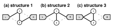
Figure 2: Three structures investigated, in which the solid and dash lines stand for the stronger and weaker tunnel coupling, respectively.

Three configurations for the DQD system according to the asymmetric couplings between two dots and leadskonig that we focus on are shown in Fig.2: (a)structure 1, in which $\Gamma^{L}_{1}=\Gamma^{R}_{2}=2\Gamma^{L}_{2}=2\Gamma^{R}_{1}=\gamma$; (b) structure 2, in which $\Gamma^{L}_{1}=\Gamma^{R}_{1}=2\Gamma^{L}_{2}=2\Gamma^{R}_{2}=\gamma$; and (c) structure 3, where $\Gamma^{L}_{1}=\Gamma^{L}_{2}=2\Gamma^{R}_{1}=2\Gamma^{R}_{2}=\gamma$. Here the $\gamma$ is taken as an energy unit. These typical structures for the DQD system are basic, yet convenient to analyze theoretically.

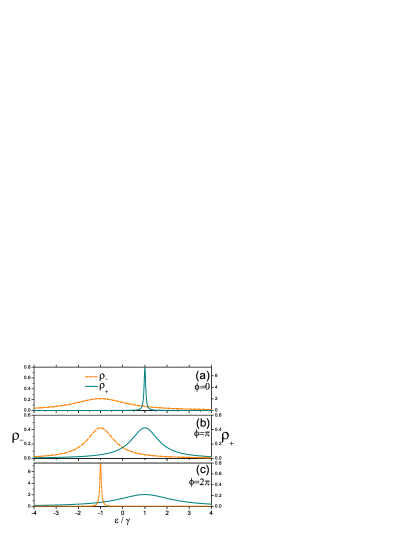
Figure 3: (Color online)The density of states for two molecular states in structure 1 and structure 2 as shown in Fig.2, where $t_{c}=\gamma$ which is taken as an energy scale.

Fig.3 shows how the calculated DOS of two molecular states changes with the total magnetic flux $\phi$ in the structure 1 and 2. It is noticed that the structure 1 and 2 share the identical DOS. Two points are worth to pointing out. Firstly, since the full width at half maximum $2\Gamma_{\pm}$ for each molecular state depends on the parameters $\Gamma^{\alpha}_{i}$, $\phi$, and $\theta$, the broadenings of molecular states could be tuned not only by the dot-lead coupling strength and total magnetic flux, but also by the flux difference. Secondly, the broadening of one molecular state is always accompanied by the shrinking of the other molecular state because the trace of the matrix of $(\widetilde{\mathbf{\Gamma}}^{L}+\widetilde{\mathbf{\Gamma}}^{R})$ is an invariant, as explicitly shown by Eqs. (11) and (12). Thirdly, in the absence of the magnetic flux ($\phi=0$), $\Gamma_{+}\rightarrow 0^{+}$ in the structure 3, i.e. the antibonding state is totally decoupled from the leads and possesses an infinite lifetime. The finite $\phi$ introduced by the magnetic flux in this structure results in the finite coupling between the antibonding state and leads, and thus a finite width for the antibonding state.

III Conductance

To study the transport through the DQD system, the conductance at zero temperature is derived, which, on the basis of the non-interacting molecular levels, can be reduced to the Landauer-Büttiker formula datta

$$\mathcal{G}(\varepsilon)=\frac{2e^{2}}{h}T(\varepsilon),$$ (16)

where, $\varepsilon$ is the Fermi energy at both leads at equilibrium. In the absence of Coulomb interaction between the electrons on the dots, the transmission $T(\varepsilon)$ is expressed asmeir

$$T(\varepsilon)=\mathrm{Tr}[\mathbf{G}^{a}(\varepsilon)\mathbf{\Gamma}^{R}\mathbf{G}^{r}(\varepsilon)\mathbf{\Gamma}^{L}],$$ (17)

where the retarded and advanced Green functions, $\mathbf{G}^{r}$ and $\mathbf{G}^{a}$, and the linewidth matrices $\mathbf{\Gamma}^{L(R)}$ can be expressed in molecular states representation or in dot levels representation, respectively.

The retarded Green function in the dot level representation is defined as $G^{r}_{ij}=-i\theta(t)\langle\{d_{i}(t),d^{\dagger}_{j}\}\rangle$, and its Fourier transformation $G^{r}_{ij}(\varepsilon)\equiv\langle\langle d_{i}|d^{\dagger}_{j}\rangle\rangle$ satisfies

$$\langle\langle d_{i}|d^{\dagger}_{j}\rangle\rangle=\delta_{ij}+\langle\langle[d_{i},H]|d^{\dagger}_{j}\rangle\rangle,$$ (18)

which generates a closed set of linear equations for $G^{r}_{ij}(\varepsilon)$. The solution of $\mathbf{G}^{r}$ is given by

$$\mathbf{G}^{r}(\varepsilon)=$$

$$\left(\begin{array}[]{cc}\varepsilon-\varepsilon_{1}+\frac{i}{2}(\Gamma^{L}_{11}+\Gamma^{R}_{11})&t_{c}+\frac{i}{2}(\Gamma^{L}_{12}+\Gamma^{R}_{12})\\ t_{c}^{*}+\frac{i}{2}(\Gamma^{L}_{21}+\Gamma^{R}_{21})&\varepsilon-\varepsilon_{2}+\frac{i}{2}(\Gamma^{L}_{22}+\Gamma^{R}_{22})\\ \end{array}\right)^{-1}.$$ (21)

The advanced Green function is the Hermite conjugate of the retarded Green function. Put Eq.(III) into Eq.(17) and after some algebra, the transmission probability through the DQD system is found to be

$$T(\varepsilon)=\frac{a(\varepsilon-\varepsilon_{0})^{2}+b(\varepsilon-\varepsilon_{0})+c}{\{[\varepsilon-(\varepsilon_{0}+t_{c})]^{2}+\Gamma^{2}_{+}\}\{[\varepsilon-(\varepsilon_{0}-t_{c})]^{2}+\Gamma^{2}_{-}\}},$$

where

$$a = \Gamma^{L}_{1}\Gamma^{R}_{1}+\Gamma^{L}_{2}\Gamma^{R}_{2}+2\cos\phi\sqrt{\Gamma^{L}_{1}\Gamma^{R}_{1}\Gamma^{L}_{2}\Gamma^{R}_{2}},$$

$$b = -2t_{c}(\Gamma^{L}_{1}+\Gamma^{L}_{2})\sqrt{\Gamma^{R}_{1}\Gamma^{R}_{2}}\cos(\theta+\frac{\phi}{2})$$

$$-2t_{c}(\Gamma^{R}_{1}+\Gamma^{R}_{2})\sqrt{\Gamma^{L}_{1}\Gamma^{L}_{2}}\cos(\theta-\frac{\phi}{2}),$$

$$c = t_{c}^{2}(\Gamma^{L}_{1}\Gamma^{R}_{2}+\Gamma^{L}_{2}\Gamma^{R}_{1}+2\cos 2\theta\sqrt{\Gamma^{L}_{1}\Gamma^{L}_{2}\Gamma^{R}_{1}\Gamma^{R}_{2}}\ ).$$

The conductance through the DQD system as expressed in Eq.(III) depends in general on the energy levels of two dots, dot-lead coupling, inter-dot coupling, and phase shift induced by the magnetic flux. Without the magnetic flux, i.e. $\phi=0$, and $\theta=0$, Eq.(III) recovers to the result by Guevara et al.guevara ; while in the limit of vanishing inter-dot coupling ($t_{c}=0$), the result of Kubala et al.kubala is repeated.

In the molecular state representation, the total conductance can also be divided into

$$\mathcal{G}_{\mathrm{total}}(\varepsilon)=\frac{2e^{2}}{h}\{T_{+}+T_{-}+T_{\mathrm{inter}}\},$$ (25)

where the transmission via each molecular state is

$$T_{\pm}(\varepsilon)=\frac{\widetilde{\Gamma}^{L}_{\pm\pm}\widetilde{\Gamma}^{R}_{\pm\pm}}{[\varepsilon-(\varepsilon_{0}\pm t_{c})]^{2}+\Gamma_{\pm}^{2}},$$ (26)

and the interference term is given by

$$T_{\mathrm{inter}}=2\mathrm{Re}\{\frac{\widetilde{\Gamma}^{R}_{+-}\widetilde{\Gamma}^{L}_{-+}}{[\varepsilon-(\varepsilon_{0}+t_{c})-i\Gamma_{+}][\varepsilon-(\varepsilon_{0}-t_{c})+i\Gamma_{-}]}\}.$$

IV Tunable Fano effect

As shown in Fig.4, the total conductance through the parallel-couple DQD system consists of a Breit-Wigner peak and a Fano peak, which is quite different from the DOS where two Lorentzians are superposed. Based on the molecular level representation formulated above, let us first explain how the Fano interference is produced in somewhat details, then show how to tune it. Although similar observations have been reported in Refs.kang, ; guevara, ; guevara2, ; baizhiming, , it seems that till now no simple and transparent explanation is available on the formation of the Fano lineshape in this structure.

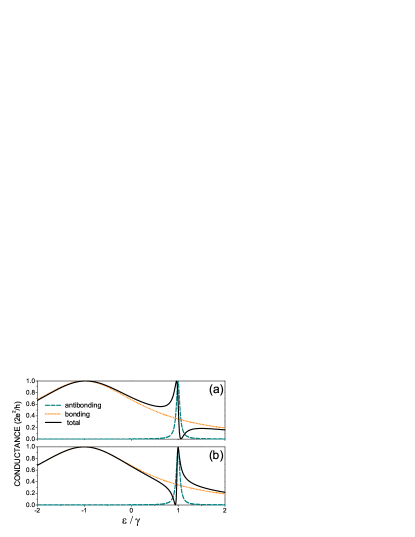
Figure 4: (Color online)Conductance spectra in structure 1(a) and structure 2(b). The parameters for calculations are $\theta=0,\phi=0,\varepsilon_{0}=0$, and $t_{c}=\gamma$. Notice that the conductance spectra in two structures have quite different interference pattern though the identical DOS as in Fig.3.

When a discrete level is buried into a continuum, the coupling between the discrete and continuous states gives rise to the renormalization of the states of whole system. The phase of the renormalized wave function varies by $\sim\pi$ swiftly as the energy transverses an interval $\sim\Gamma$ around the discrete level, where $\Gamma$ is the broadening of the discrete level due to coupling with the continua.fano ; mahan Then, if there is a reference channel whose phase changes little in the interval of $\Gamma$ around the discrete level, the quantum interference above and below the resonance level will be responsible for the Fano lineshape in the conductance spectra, for example, the experimentally observed Fano lineshape in the hybrid system of a QD and a reference arm.Kobayashi2002 ; Kobayashi2003 ; johnson

In the present DQD multi-path system, it is not simple to identify the resonant and the reference channel. But, on the basis of the molecular level representation, it is straightforward to interpret the Fano resonance in the DQD system in terms of the interference between two channels.

Usually, two molecular levels are coupled to the leads unequally. In the absence of magnetic flux, Eq.(14) simply reduces to

$$\Gamma_{\pm}=\frac{1}{4}(\Gamma^{L}_{1}+\Gamma^{L}_{2}+\Gamma^{R}_{1}+\Gamma^{R}_{2})\mp\frac{1}{2}(\sqrt{\Gamma^{L}_{1}\Gamma^{L}_{2}}+\sqrt{\Gamma^{R}_{1}\Gamma^{R}_{2}}),$$ (28)

i.e., the broadening of one level is always accompanied by the shrinking of the other. The molecular level associated with a wider band can be referred to as the strongly-coupled one, while that with narrow band is referred to as the weakly-coupled level. Suppose that the broadening of the strongly-coupled level entirely covers the band width with the weakly-coupled level, and the phase shift for the strongly-coupled channel is negligibly small around the weakly-coupled level, then a phase shift of $\pi$ across the weakly-coupled level can be detected with characteristic of the Fano lineshape. Namely, the waves through two channels interfere constructively for electron with energy on one side of the weakly-coupled level; while interfere destructively on the other side. As a result, the Fano lineshape shows up around the weakly-coupled state. It is worth pointing out that the $\pi$ phase shift also happens around the strongly-coupled level, but on a energy scale much larger than that around the weakly-coupled level (Fig.3). That is why usually there is only one Fano peak around the weakly-coupled level, and the other peak around the strongly-coupled level only exhibits little asymmetry.

Compared with the Fano effect in the hybrid system,Kobayashi2002 ; Kobayashi2003 ; johnson where the nonresonant channel served by a quantum point contact detects the $\pi$ phase shift around the resonant tunneling channel through the QD, in the DQD system, the reference channel is the ”less resonant” tunneling channel on one side of the strongly-coupled level, and the other ”more resonant” channel through the weakly-coupled level is accompanied with a swift $\pi$ phase shift within a small energy region.

The Fano lineshape in the present system can be tuned by the applied electrostatic and magnetic fields. Compared with the one dot and one arm case, where the magnetic field affects only the phase of the electron, but not the interaction strength,Kobayashi2002 ; Kobayashi2003 in the parallel-coupled DQD, not only the phase but also the magnitude of the effective coupling between the molecular states and leads can be tuned by the magnetic flux. Of course, one should keep in mind that the inter-dot coupling is the prerequisite to the tunable Fano effect.

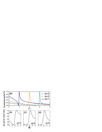
Figure 5: (Color online)(a)Calculated conductance in the structure 2 for three different values of inter-dot coupling $t_{c}$, where the Fermi energy is roughly at the antibonding level. (b),(c),and (d) Simulation of the normalized Fano lineshape with different asymmetric factors $q$ as compared to the results obtained by Green functions in (a).

IV.1 Electrostatic tuning

The inter-dot coupling $t_{c}$ can be tuned by adjusting the height and thickness of the tunneling barrier between two dots through gate voltages. So can be done the dot-lead coupling $\Gamma^{L(R)}_{i}$.

The interference between the resonance and the reference channels can be described as

$$|t_{R}\frac{\Gamma}{\omega-\epsilon_{0}+i\Gamma}+t_{N}e^{i\phi}|^{2}=t^{2}_{N}\frac{|\widetilde{\epsilon}+q|^{2}}{\widetilde{\epsilon}^{2}+1},$$ (29)

where $t_{R}$ and $t_{N}$ denote respectively the transmission amplitude via the resonance and the reference channels, the detuning $\widetilde{\epsilon}=(\omega-\epsilon_{0})/\Gamma$, and the asymmetric factor $q=i+t_{R}e^{-i\phi}/t_{N}$. It is well known that when the asymmetric factor $q$ is small, Eq.(29) gives rise to the asymmetric Fano lineshape; while for large $q$, it tends to the symmetric Lorentzian. Fig. 5(a) depicts the conductance spectra for three different inter-dot coupling strengths in Structure 2. As for comparison, the normalized Fano lineshape (multiplied by a normalized factor $1/(1+q^{2})$) is also plotted in Fig.5(b),(c), and (d), demonstrating how the Fano lineshape evolves with increasing $q$. It is obvious that as the inter-dot coupling increases, the bonding and antibonding splitting increases. As a result, the amplitude through the channel associated with the strongly-coupled level but at the energy range of antibonding peak, $t_{N}$, decreases, and since $q$ is inversely proportional to $t_{N}$, the asymmetric factor $q$ increases. This further confirms our explanation above about the origin of Fano effect in this parallel-coupled DQD system.

When tuning the dot-lead coupling strength $\Gamma^{L(R)}_{i}$ by tuning the gate voltage, the structure studied is changed, and the Fano lineshape is changed accordingly. For example, when the strong and weak coupling in the linewidth matrix is adjusted such that the structure 1 is transformed into the structure 2, (see Fig.4b), noticeably, the tail direction of the Fano peak is flipped. This delicate change can be understood in terms of the product of the effective tunneling matrix elements

$$\widetilde{V}_{L+}\widetilde{V}^{*}_{R+}\widetilde{V}_{R-}\widetilde{V}^{*}_{L-}$$

$$= \frac{1}{4}(V_{L1}-V_{L2})(V_{R1}-V_{R2})(V_{L1}+V_{L2})(V_{R1}+V_{R2}).$$

In the wide band limit, a linewidth matrix element is proportional to the product of two dot-lead tunneling matrix elements. According to Fig.2, the expression above for the structure 1 differs from that for structure 2 by a minus sign, which implies that, compared to structure 2, an extra flux of $\pi$ threads the loop in the structure 1(Fig.6). Thus, the Fano lineshape in structure 1 is just opposite to that in structure 2, i.e., if two channels interfere with each other constructively in structure 1, then destructively in structure 2; and vice versa.

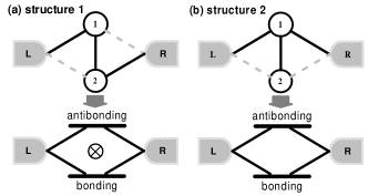
Figure 6: (a) Structure 1 and (b)structure 2 can be cast into two different models of molecular states. The flux through the loop of structure 1 differs from that of structure 2 by a phase of $\pi$.

IV.2 Magnetic flux tuning and swap operation

Coupled quantum dot systems have been proposed to materialize quantum bit for quantum computationloss . The swap operation is an important element to the controlled-NOT gate, which is the key to implementing the quantum computation. divincenzo Recently, a new mechanism has been proposed to realize the swap operation in the parallel-coupled DQD system by using the time-dependent inter-dot spin superexchange J(t), which flips the singlet and triplet states formed by two localize electrons.zhang In the following we will discuss a new type of swap operation in the DQD system, which flips two quantum states by tuning the magnetic flux, including tuning the total flux $\phi$ or the flux difference $2\theta$ between the left and right sub-rings. For the purpose of comparison, only tuning one parameter, and letting the other alone.

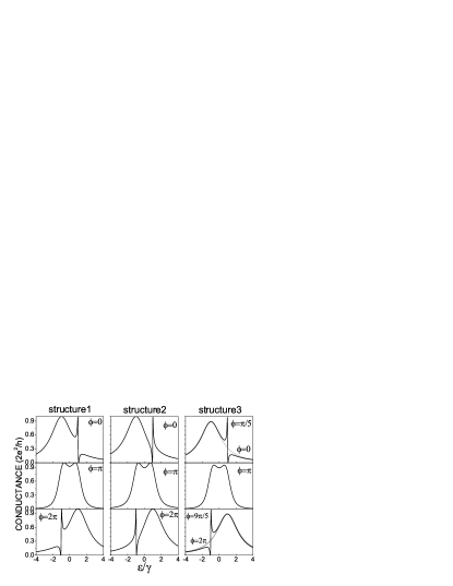
Figure 7: The evolution of transmission spectrum with total magnetic flux $\phi$ tuned for three asymmetric configurations.

First, we tune the total flux $\phi$ and let $\theta=0$. When $\phi=(2n+1)2\pi$ (n is an integer), Eq.(14) turns out to be $\Gamma_{\pm}=\frac{1}{4}(\Gamma^{L}_{1}+\Gamma^{L}_{2}+\Gamma^{R}_{1}+\Gamma^{R}_{2})\pm\frac{1}{2}(\sqrt{\Gamma^{L}_{1}\Gamma^{L}_{2}}+\sqrt{\Gamma^{R}_{1}\Gamma^{R}_{2}}).$ Compared with the case of null flux, or $\phi=4n\pi$[ Eq.(28)], the widths of the bonding and antibonding states are interchanged. Fig.7 demonstrates the evolution of conductances with changing the total magnetic flux in three asymmetric configurations for zero $\theta$. In this circumstance the Fano and Breit-Wigner peaks in the conductance spectra of the structures 1 and 2 have been exchanged each other, when changing $\phi$ from $(2n+1)2\pi$ to $\phi=4n\pi$. On the other hand, when $\phi=(2n+1)\pi$, two identical peaks appear in conductance spectra symmetrically, which is quite similar to the DOS spectra. In structure 3, no Fano peak exists without the magnetic flux according to Eq.(15) and Fig.7, because the antibonding state is totally decoupled from the leads. However, if $\phi$ deviates a little from zero, or more generally, from a multiple of $2\pi$, the channel connecting the decoupled state and the leads is open, and the Fano interference comes back again. Our model calculation indicates that, this flux-dependent Fano effect takes place whenever $\Gamma^{L}_{1}=\Gamma^{L}_{2}$ and $\Gamma^{R}_{1}=\Gamma^{R}_{2}$, regardless whether four dot-lead couplings are the identical.guevara

Tuning $\theta$, the half of the flux difference between the left and right sub-rings, can also lead to two resonance peak swap and the flux-dependent Fano effect as shown in Fig.8. It is noticed when $\theta=\pi$, the results coincide with what obtained when $\phi=2\pi$.

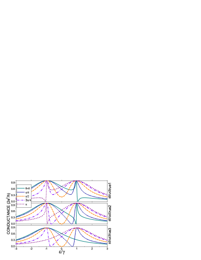
Figure 8: (Color online)The evolution of transmission spectrum with phase difference $\theta$ in three asymmetric configurations.

It is interesting to note that the conductance oscillation is a periodic function of $\phi$ with a period of $4\pi$, and a periodic function of $\theta$ with the period of $2\pi$. The difference in the period can be readily explained as the multi-pathway nature in this parallel-coupled DQD system. If an electron transits from the left to the right, it gathers a phase factor $e^{i(\frac{\phi}{4}+\frac{\phi}{4})}=e^{i\frac{\phi}{2}}$ via the upper arms and $e^{-i\frac{\phi}{2}}$ via the lower arms(Fig.9a). The interference of the two paths gives $\cos\frac{\phi}{2}$, which is associated with a period of $4\pi$. On the other hand, if two routes of an electron are illustrated as the arrows in Fig.9b, the interference yields $\cos{\theta}$ and the $2\pi$ periodicity, because the first path from the left lead $\rightarrow$ dot 1 $\rightarrow$ dot 2 $\rightarrow$ right lead accumulates a phase $e^{i(\frac{\phi}{4}+\theta-\frac{\phi}{4})}=e^{i\theta}$, and the second symmetric route through dot2 $\rightarrow$ dot1 gives a phase $e^{-i\theta}$.

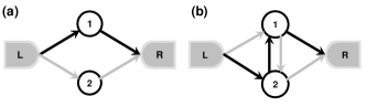
Figure 9: Illustration for two different periods of conductance. Multi-pathway interference as functions of (a) the total flux $\phi$, and (b) the flux difference $\theta$.

The quantum interference tuned by the magnetic flux in the DQD system makes the conductance to vary in some fancy way. Let us look at a peculiar instance, the continuous manipulation of the conductance with the lineshape retained. In Fig.10, two cases of the flux tuning are: (1) $\phi=(2n+1)\pi$, $\theta\in[0,\frac{\pi}{2}]$; and (2) $\theta=(2n+1)\frac{\pi}{2}$, $\phi\in[0,\pi]$. According to Eq.(11) and Eq.(12), once $\theta=(2n+1)\frac{\pi}{2}$ or $\phi=(2n+1)\pi$, the lineshape of the DOS for two molecular levels is fixed. In our calculations, $\Gamma^{L}_{1}=\Gamma^{L}_{2}=\Gamma^{R}_{1}=\Gamma^{R}_{2}=t_{c}=\gamma,\ \varepsilon_{0}=0$, only a single peak appears in Fig.10(a)(when increasing $t_{c}$, the conductance will recover the double-peak feature). In contrast, in Fig.10(b) due to the destructive interference, the conductance at $\varepsilon_{0}$ is always zero. Besides, a fully symmetric configuration with four identical dot-lead couplings is considered in this calculation, so that the maximum and minimum values of the conductance are precisely at $2e^{2}/h$ and 0, respectively.

Figure 10: Continuously modulated conductance by the magnetic flux. (a) The conductance is tuned by $\theta$, when $\phi$ is fixed at $(2n+1)\pi$; (b) The conductance is tuned by $\phi$, when $\theta=(2n+1)\frac{\pi}{2}$.

V Conclusions

In summary, the transport through the parallel-coupled DQD system has been studied, in which a particular attention is paid to the mechanism of the Fano lineshape in conductance spectra as well as its tunability. Due to the inter-dot coupling, a QD-molecule is formed and can be the proper representation for the present investigations. Due to the coupling between the molecular levels and leads, two levels are broadened into two bands: one is wider which is associated with the strongly-coupled level, and the other is narrower band related to the weakly-coupled level. When the wider band covers the narrower band, and the phase shift of the wavefunction of the wider band is negligible around the weakly-coupled level, the $\pi$ phase shift at resonance of the wavefunction of the narrower band may be detected via the quantum interference, and shows up as the Fano lineshape. Thus, both the reference and the resonance channels for Fano interference are readily identified. Since the density of states and the effective couplings between the molecular levels and leads are tunable by making use of the magnetic flux and gate-voltages, several ways to control Fano lineshape are proposed, including the total flux $\phi$, the flux difference between two sub-rings $\theta$, the inter-dot coupling strength $t_{c}$, and the dot-lead coupling. In these ways, we may realize the swap effect, the flipped tail direction of the Fano lineshape, and the continuous lineshape-keeping magnetic switch in this DQD system, which might be of practical applications.

- (1) L.P. Kouwenhoven, C.M. Markus, P.L. McEuen, S. Tarucha, R.M. Westervelt, and N.S. Wingreen, in Mesoscopic Electon Transport, edited by L.L. Sohn, L.P. Kouwenhoven, and G. Schn, NATO Advanced Study Institutes, Ser. E, Vol. 345 (Kluwer, Dordrecht, 1997).
- (2) Y. Aharonov and D. Bohm, Phys. Rev. 115, 485 (1959).
- (3) A.W. Holleitner, C.R. Decker, H. Qin, K. Eberl, and R.H. Blick, Phys. Rev. lett. 87, 256802 (2001).
- (4) A.W. Holleitner, R.H. Blick, A.K. Hüttel, K. Eberl, and J.P. Kotthaus, Science 297, 70 (2002).
- (5) A.W. Holleitner, R.H. Blick, and K. Eberl, Appl. Phys. Lett. 82, 1887 (2003).
- (6) R.H. Blick, A.K. Hüttel, A.W. Holleitner, E.M. Höhberger, H. Qin, J. Kirschbaum, J. Weber, W. Wegscheider, M. Bichler, K. Eberl, and J.P. Kotthaus, Physica E 16, 76 (2003).
- (7) A. Yacoby, M. Heiblum, D. Mahalu, and H. Shtrikman, Phys. Rev. Lett. 74, 4047 (1995).
- (8) R. Schuster, E. Buks, M. Heiblum, D. Mahalu, V. Umansky, and H. Shtrikman, Nature(London) 385, 417 (1997).
- (9) E. Buks, R. Schuster, M. Heiblum, D. Mahalu ,and V. Umansky, Nature(London) 391, 871 (1998).
- (10) W.G. van der Wiel, S. De Franceschi, T. Fujisawa, J.M. Elzerman, S. Tarucha, and L.P. Kouwenhoven, Science 289, 2105 (2000).
- (11) Y. Ji, M. Heiblum, D. Sprinzak, D. Mahalu, H. Shtrikman, Science 290, 779 (2000).
- (12) K. Kobayashi, H. Aikawa, S. Katsumoto, and Y. Iye, Phys. Rev. Lett. 88, 256806 (2002).
- (13) K. Kobayashi, H. Aikawa, S. Katsumoto, and Y. Iye, Phys. Rev. B 68, 235304 (2003).
- (14) J. Göres, D. Goldhaber-Gordon, S. Heemeyer, M.A. Kastner, H. Shtrikman, D. Mahalu, and U. Meirav, Phys. Rev. B 62, 2188 (2000).
- (15) I.G. Zacharia, D. Goldhaber-Gordon, G. Granger, M.A. Kastner, Y.B. Khavin, H. Shtrikman, D. Mahalu, and U. Meirav, Phys. Rev. B 64, 155311 (2001).
- (16) A.C. Johnson, C.M. Marcus, M.P. Hanson, and A.C. Gossard, Phys. Rev. Lett. 93, 106803 (2004)
- (17) U. Fano, Phys. Rev. 124, 1866 (1961).
- (18) R.K. Adair, C.K. Bockelman, and R.E. Peterson, Phys. Rev. 76, 308 (1949).
- (19) U. Fano and J.W. Cooper, Phys. Rev. 137, A1364 (1965).
- (20) F. Cerdeira, T.A. Fjeldly, and M. Cardona, Phys. Rev. B 8, 4734 (1973).
- (21) J. Faist, F. Capasso, C. Sirtori, K.W. West, and L.N. Pfeiffer, Nature (London) 390, 589 (1997).
- (22) F.R. Waugh, M.J. Berry, D.J. Mar, R.M. Westervelt, K.L. Campman, and A.C. Gossard, Phys. Rev. Lett. 75, 705 (1995).
- (23) R.H. Blick, D. Pfannkuche, R.J. Haug, K.v. Klitzing, and K. Eberl, Phys. Rev. Lett. 80, 4032 (1998).
- (24) T.H. Oosterkamp, T. Fujisawa, W.G. van der Wiel, K. Ishibashi, R.V. Hijman, S. Tarucha, and L.P. Kouwenhoven, Nature (London) 395, 873 (1998).
- (25) H. Qin, A.W. Holleitner, K. Eberl, and R.H. Blick, Phys. Rev. B 64, 241302(R) (2001).
- (26) J.C. Chen, A.M. Chang, and M.R. Melloch, Phys. Rev. Lett. 92, 176801 (2004).
- (27) D. Loss and D.P. DiVincenzo, Phys. Rev. A 57, 120 (1998).
- (28) X. Hu and S. Das Sarma, Phys. Rev. A 61, 062301 (2000).
- (29) D.P. DiVincenzo, cond-mat/9612126; in Mesoscopic Electron Transport, edited by L.L. Sohn, L.P. Kouwenhoven, and G. Schön, NATO Advanced Study Institutes, Ser. E, Vol. 345 (Kluwer, Dordrecht, 1997).
- (30) A.A. Clerk, X. Waintal, and P.W. Brouwer, Phys. Rev. Lett. 86, 4636 (2001).
- (31) G.D. Mahan, in Many-Particle Physics (Sencond Edition, Plenum Press, New York, 1990).
- (32) K. Kang and S.Y. Cho, J. Phys.: Condens. Matter 16, 117 (2004).
- (33) M.L. Ladrón de Guevara, F. Claro, and Pedro A. Orellana, Phys. Rev. B 67, 195335 (2003).
- (34) Z.-M. Bai, M.-F. Yang, and Y.-C. Chen, J. Phys.:Condens.Matter 16, 2053 (2004).
- (35) B. Dong, I. Djuric, H.L. Cui, and X.L. Lei, cond-mat/0403741 (2004).
- (36) P.A. Orelana, M.L. Ladrón de Guevara, and F. Claro, cond-mat/0404293 (2004).
- (37) C. Livermore, C.H. Crouch, R.M. Westervelt, K.L. Campman, and A.C. Gossard, Science 274, 1332 (1996).
- (38) H. Haug and A.-P. Jauho, Quantum Kinetics in Transport and Optics of Semiconductors (Springer-Verlag, 1996).
- (39) J. König and Y. Gefen, Phys. Rev. B 65, 045316 (2002)
- (40) S. Datta, Electronic transport in mesoscopic systems (Cambridge Univ. Press, 1997).
- (41) Y. Meir and N.S. Wingreen, Phys. Rev. Lett. 68, 2512 (1992).
- (42) B. Kubala and J. König, Phys. Rev. B 65, 245301 (2002).
- (43) D.P. DiVincenzo, Phys. Rev. A 51, 1015 (1995).
- (44) G.-M. Zhang, R. Lü, Z.R. Liu, and L. Yu, cond-mat/0403629.