Evolution in complex systems:
record dynamics in models of spin glasses, superconductors and evolutionary ecology.

Abstract

Recent research on the non-stationary nature of the dynamics of complex systems is reviewed through three specific models. The long time dynamics consists of a slow, decelerating but spasmodic release of generalized intrinsic strain. These events are denoted quakes. Between the quakes weak fluctuations occur but no essential change in properties are induced. The accumulated effect of the quakes, however, is to induce a direct change in the probability density functions characterising the system. We discuss how the log-Poisson statistics of record dynamics may be an effective description of the long time evolution and describe how an analysis of the times at which the quakes occur enables one to check the applicability of record dynamics.

Out of equilibrium systems are often treated as being in a stationary state characterised by time independent statistical measures. Although this is probably the case in some situations there are many instances where this is not so and where one may miss essential aspects of the behaviour if attempts are made to treat the phenomena as stationary or nearly stationary.

Complex systems often display evolving macroscopic properties. The most important task of a theoretical treatment is then to understand the link between the microscopic fluctuations, which will often exhibit an approximate time reversal symmetry and the macroscopic directed evolution. The description should as well explain the nature of the emergent macroscopic dynamics.

Here we review how the concept of record dynamics, developed by Sibani and Littlewood[1], has successfully served as a paradigm for the description of the evolution of three very different models: the relaxation of a spin glass following an initial temperature quench, the penetration of an external magnetic field into a disordered type II superconductor and a model of evolutionary ecology. In all three cases macroscopic variables, which exhibit a degree of intermittent dynamics, can be identified. Furthermore, the sequence of transitions between metastable configurations can be analysed in terms of the record statistics.

The work reviewed here is a result of collaboration with Paolo Sibani, Paul Anderson and Luis P Oliveria. Some details of the specifics have been published in [2, 3, 4, 5]. The concept of record dynamics have been developed by Sibani and his collaborators over a long period, see e.g. [1, 6, 7, 8, 9].

Below we first introduce the models in sufficient self-contained detail. Next we describe how the long time dynamics in each case are manifestations of record dynamics and discuss its consequences.

I Three models

Here follows a brief description of the definition of the microscopic dynamics of the three models considered.

I.1 Spin glass

We consider a three dimensional Edwards-Anderson spin glass

$$H=-\frac{1}{2}\sum_{\langle ij\rangle}J_{ij}S_{i}S_{j}.$$ (1)

with nearest neighbour Gaussian couplings[10] and Ising spin $S_{i}=\pm 1$. At time zero the temperature is instantaneously dropped from infinity to a very low value. The subsequent dynamics is realised by use of Monte Carlo dynamics, see [3, 4, 8].

I.2 Magnetic relaxation

We use Monte Carlo (MC) simulations of a generalized three dimensional layered version of the Restricted Occupancy Model (ROM) model to capture the long time relaxation of interacting vortex matter [11, 12, 13, 14, 15, 16, 5].

The length scales of vortex interactions can be very large compared with the average separation between vortices. At high magnetic induction each vortex interacts with many others suggesting that a simplified coarse grained description in terms of vortex densities may be applicable. For layered superconductors it is natural to introduce two separate length scales: the first is the range of the interaction parallel to the planes, this is the London penetration depth $\lambda$. The second length scale is the vortex correlation length, $\xi_{||}$, parallel to the applied field (which we imagine to be perpendicular to the copper oxide planes for high temperature superconductors). The exact identification of this length scale is difficult and is likely to depend on the anisotropy of the material, the nature of the pinning, the strength of the magnetic induction and on the temperature. This length scale may be related to vortex line cutting[17, 18, 19, 20, 21, 22, 23, 24]. These length scales respectively give the horizontal, $l_{0}$, and vertical, $l_{1}$, coarse-graining length and therefore the lattice spacing of our model. Horizontally we have $l_{0}=\lambda$ and perpendicularly $l_{1}\sim\xi_{||}$. Smaller length scales are ignored. For our purposes this approximation is acceptable because the length scales smaller than $\lambda$ seem to have little influence on the long time glassy properties of vortex matter.

The behaviour of vortex matter is determined by the competition of four energy scales [25]: intra and interlayer vortex-vortex interaction, vortex-pinning interaction and thermal fluctuations, all of which are schematically included in the ROM model.

The Hamiltonian of the ROM model is thus the following:

$$H=\sum_{ij}A_{ij}n_{i}n_{j}-\sum_{i}A_{ii}n_{i}+\sum_{i}A_{i}^{p}n_{i}+\sum_{\left\langle ij\right\rangle_{z}}A_{2}\left(n_{i}-n_{j}\right)^{2},$$ (2)

where $n_{i}$ is the number of vortices on site $i$ of the lattice. In a superconducting sample the number of vortex lines per unit area is restricted by the upper critical field ($B_{c2}$) [26], so in the model the number of vortices per cell can only assume values smaller than $N_{c2}=B_{c2}l_{0}^{2}/\phi_{0}$ [27, 14]. Hence the name Restricted Occupancy Model. Moreover, as we are interested in a simulation setup that does not require magnetic field inversion and the vortex-antivortex creation is strongly suppressed, we simply consider $n_{i}\geq 0$.

The first two terms in Eq. (2) represent the repulsion energy due to vortex-vortex interaction in the same layer, and the vortex self energy respectively. Since the potential that mediates this interaction decays exponentially at distances longer than our coarse-graining length $\lambda$, interactions beyond nearest neighbours are neglected. We set $A_{ii}:=A_{0}=1$, $A_{ij}:=A_{1}$ if $i$ and $j$ are nearest neighbours on the same layer, and $A_{ij}:=0$ otherwise.

The third term represents the interaction of the vortex pancakes with the pinning centres. $A_{i}^{p}$ is a random potential and for simplicity we consider that $A_{i}^{p}$ has the following distribution $P\left(A_{i}^{p}\right)=\left(1-p\right)\delta\left(A_{i}^{p}\right)-p\delta\left(A_{i}^{p}-A_{0}^{p}\right)$. The pinning strength $\left|A_{0}^{p}\right|$ represents the total action of the pinning centres located on a site. In the present work we use $\left|A_{0}^{p}\right|=0.3$.

Finally the last term describes the interactions between the vortex sections in different layers. This term is a nearest neighbour quadratic interaction along the $z$ axis, so that the number of vortices in neighbouring cells along the $z$ direction tends to be the same.

The parameters of the model are defined in units of $A_{0}$. The time is measured in units of full MC sweeps. The relationship between the model parameters and material parameters is discussed in [27, 14]. The model has been demonstrated to reproduce a very broad range of experimental observations including dynamical aspects of magnetic creep and memory and rejuvenation of voltage-current characteristics[28, 11, 12, 13, 14, 15, 16].

Each individual MC update involves the movement to a neighbour site of a single randomly selected vortex. The movement of the vortex is automatically accepted if the energy of the system decreases; if the energy of the system increases, the movement is accepted with probability $\exp(-\Delta E/T)$ [29].

The external magnetic field is modelled by the edge sites on each of the planes. The density at the edge is kept at a controlled value. During a MC sweep vortices may move between the bulk sites and the edge sites. After each MC sweep the density on the edge sites is brought to the desired value. Initially the external field is increased to a desired value ($N_{ext}=10$ vortices per edge site) by a very rapid increase in the density on the edge sites.

After this fast initial ramping the external field is kept constant, while we study how the vortices move into the sample. The age of the system, $t_{w}$, is taken to be the time since the initial ramping.

I.3 Tangled Nature

I.4 Definition of the model

The Tangled Nature model is an individual based model of evolutionary ecology. We give a brief outline of the model here. Details can be found in [30, 31, 2]. An individual is represented by a vector ${\bf S}^{\alpha}=(S_{1}^{\alpha},S_{2}^{\alpha},...,S_{L}^{\alpha})$ in the genotype space $\cal{S}$, where the “genes” $S^{\alpha}_{i}$ may take the values $\pm 1$, i.e. ${\bf S}^{\alpha}$ denotes a corner of the $L$-dimensional hypercube. In the present paper we take $L=20$ as this gives space of a reasonable size to explore (over a million genotypes) whilst not being computationally prohibitive. We think of the genotype space $\cal{S}$ as containing all possible ways of combining the genes into genome sequences. Many sequences may not correspond to viable organisms. The viability of a genotype is determined by the evolutionary dynamics. All possible sequences are made available for evolution to select from. The number of occupied sites is referred to as the diversity, here analogous to the number of species or species richness [32]. As explained later, genotype, species, site and node are synonymous throughout.

For simplicity, an individual is removed from the system with a constant probability $p_{kill}$ per time step. A time step consists of one annihilation attempt followed by one reproduction attempt. One generation consists of $N(t)/p_{kill}$ time steps, which is the average time taken to kill all currently living individuals. All references to time will be in units of generational time.

The ability of an individual to reproduce is controlled by a weight function $H({\bf S}^{\alpha},t)$:

$$H({\bf S}^{\alpha},t)={1\over cN(t)}\left(\sum_{{\bf S}\in{\cal S}}J({\bf S}^{\alpha},{\bf S})n({\bf S},t)\right)-\mu N(t),$$ (3)

where $c$ is a control parameter, $N(t)$ is the total number of individuals at time $t$, the sum is over the $2^{L}$ locations in ${\cal S}$ and $n({\bf S},t)$ is the number of individuals (or occupancy) at position ${\bf S}$. Two positions ${\bf S}^{a}$ and ${\bf S}^{b}$ in genome space are coupled with the fixed random strength $J^{ab}=J({\bf S}^{a},{\bf S}^{b})$ which can be either positive, negative or zero. This link is non-zero with probability $\theta$, i.e. $\theta$ is simply the probability that any two sites are interacting. To study the effects of interactions between species, we exclude self-interaction so that $J^{aa}=0$.

The conditions of the physical environment are simplistically described by the term $\mu N(t)$ in equation (3), where $\mu$ determines the average sustainable total population size, i.e. the carrying capacity of the environment. An increase in $\mu$ corresponds to harsher physical conditions. Notice that genotypes only adapt to each other and the physical environment represented by $\mu$. We use asexual reproduction consisting of one individual being replaced by two copies mimicking the process of binary fission seen in bacteria. Successful reproduction occurs with a probability per unit time given by

$$p_{off}({\bf S}^{\alpha},t)={\exp[H({\bf S}^{\alpha},t)]\over 1+\exp[H({\bf S}^{\alpha},t)]}\in[0,1].$$ (4)

This function is chosen for convenience. We simply need a smoothly varying function that maps $H({\bf S}^{\alpha},t)$ to the interval $[0,1]$ and it is otherwise arbitrary. We allow for mutations in the following way: with probability $p_{mut}$ per gene we perform a change of sign $S_{i}^{\alpha}\rightarrow-S_{i}^{\alpha}$ during reproduction.

Initially, we place $N(0)=500$ individuals at randomly chosen positions. Their initial location in genotype space does not affect the nature of the dynamics. A two-phase switching dynamic is seen consisting of long periods of relatively stable configurations (quasi-Evolutionary Stable Strategies or q-ESSs) interrupted by brief spells of reorganisation of occupancy which are terminated when a new q-ESS is found, as discussed in [30].

II Record dynamics and its manifestation

In this section we review the macroscopic intermittent dynamics of the three models and show that in all cases record dynamics is an efficient description of the statistical aspects of the temporal evolution. Before that we need to sketch the notion of record statistics.

Let $\chi(t)$ denote an uncorrelated stochastic signal distributed according to the probability density function(pdf) $p(\chi)$. By the record of the signal we mean $R(t)={\rm max}\{\chi(t^{\prime})|t^{\prime}\leq t\}$. Obviously $R(t)$ is a piecewise constant function which jumps discontinuously as a fluctuation manages to take $\chi(t)$ to a new record value. The times $t_{k}$ at which this happens are called the record times. It was pointed out be Sibani and Littlewood[33] that the probability that exactly $q$ records occure during a time interval $[t_{w},t_{w}+t]$ is to a good approximation given by

$$p(q)=\frac{\langle q\rangle^{q}}{q!}\exp\{-\langle q\rangle\},$$ (5)

where $\langle q\rangle=\alpha\log(1+t/t_{w})$. This is a Poisson distribution in the logarithm of time. For a mathematical process the logarithmic rate $\alpha=1$. Here we include the possibility $\alpha\neq 1$, which may happen for a physical process as an effect of over or undercounting of the true number of records. For example $\alpha>1$ can occur if the recorded record times are produced by more than a single independent record process. In contrast $\alpha<1$ can e.g. be an effect of not being able resolve all the record events of record process. The average number of records per time unit decreases inversely proportional with time, namely

$$\frac{d\langle q\rangle}{dt}=\frac{\alpha}{t_{w}+t}.$$ (6)

It is important to note that Eqs. (5) and (6) are independent of $p(\chi)$. Thus the statistical properties of a record signal $R(t)$ are very general and do not depend on the properties of the underlying fluctuating signal $\chi(t)$.

II.1 Spin-glass

After an initial quench from very high temperature it is natural that the dynamics of the spin glass leads to a relaxation towards ever lower energy. The specifics of how this happens was analysed in great detail by Sibani and collaborators[9, 8] for the Edwards-Anderson spin glass. They followed the temporal evolution of the total energy $E(t)$ given in Eq. (1. They identified the sequence of local minima $E_{min}(k)$ and local maxima $E_{max}(k)$ from which they defined the $k$-th barrier as $\Delta E_{k}=E_{m}ax(k)-E_{m}in(k)$. The set of barriers turn out to be monotonously increasing $\Delta E_{k}<\Delta E_{k+1}$, but only marginally so in the sense that $\Delta E_{k}\simeq\Delta E_{k+1}$. Thus to exit the $k$-th metastable state visited by the spin glass, a barrier slightly larger than any encountered previously has to be overcome. The set of time instances at which the spin glass manage to move from one metastable configuration, i.e. the quake times $t_{k}$, was found to follow the log-Poisson distributed characteristic of record statistics, see E.q. (5).

II.2 Magnetic relaxation

The magnetic pressure exerted by the external magnetic field in the ROM model introduced above will force the number of vortices in the bulk, $N_{v}(t)$, of the sample to increase with time. We have found that $N_{v}(t)$ is essentially a record signal[2, 5], see Fig. 1.

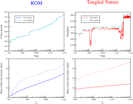
Figure 1: Time dependence of the ROM and the Tangled Nature model

The sequence of record times follow to good approximation the statistics derivable from Eq. (5) expected for an uncorrelated record signal[2].

II.3 Evolutionary Ecology

That directedness of the temporal evolution of the quenched spin glass and also of the superconductor in an external field is to be expected. It is less obvious why the Tangled Nature model of biological evolution exhibit a gradual adaptation towards more stable configurations. The diffusive nature of the dynamics in genotype space may suggest the breaking of time reversal symmetry. But this in itself doesn’t point to a reason why the total number of individuals in the model is increasing, on average, with time. Nor does diffusion imply that the configurations tend to be come more stable with time.

The following analysis suggests an explanation. First assume that no mutations can occur. The population dynamics is controlled by the fixed probability $p_{kill}$ and the offspring probability $p_{off}$. Fluctuations in the population size $N(t)$ will lead to fluctuations in $p_{off}$ according to Eq. (3). The overall stability of the population is ensured since the fixpoint condition $p_{off}=p_{kill}$ is stable. This follows because an increase in $N(t)$ will lead to a decrease in $H$ (see Eq. (3) and therefore in $p_{off}$. Similarly a decrease in $N(t)$ leads to a increase in $H$. Now consider the effect of mutations. The evolutionary dynamics is driven by the mutations which move individuals between positions in genotype space. These mutations are random and lead to symmetric fluctuations in the weight function $H$ as an effect of changing the coupling term $H$, see Eq. (3). Let us schematically write $H$ as $H={\cal J}-\mu N$. Mutations induce fluctuations of the form ${\cal J}\mapsto{\cal J}+\delta{\cal J}$. Assume $\delta{\cal J}>0$ and that the same fluctuation with opposite sign $-\delta{\cal J}$ occurs with equal probability. The mutation leading to $\delta{\cal J}$ is, however, more likely to become established since

$$p_{off}(h+\delta{\cal J})>p_{off}(H-\delta{\cal J}),$$ (7)

for values of $H$ where $p_{off}$ is convex; which is the case for $p_{off}<1/2$ according to Eq. (4). This is a mathematical way of paraphrasing Darwin’s description of how favourable variations become entrenched[34].

It was found from simulations of the Tangled Nature model that $N(t)$ gradually increases. Furthermore, the configurations occupied in genotype space becomes, on average, more stable with time[31, 2]. In Fig. 1 we compare the record signal derive from $N(t)$ with $N(t)$. It is clear that there are much larger deviations between the record and the signal itself, than was the case in the ROM model. Nevertheless, we do believe that the statistics of the record times obtained from the record signal derive from $N(t)$ essentially corresponds to the transition times between the q-ESS epochs.

III Consequences

We briefly review some of the most prominent consequences, which may be derived from the record dynamics.

III.1 Spin glasses

A detailed description of how certain aspect of intermittency, aging and memory in spin glasses can be considered a consequence of record dynamics was given in [3, 4]. That the fluctuations clearly separates into ‘quake’ fluctuations and Gaussian equilibrium like fluctuations show up directly in a study of the heat exchange between the spin glass and its thermal bath. The pdf for the heat exchange consists of a Gaussian part and an exponential tail. The exponential tail is produced by the large releases of energy that occur when a quake takes the spin glass from one metastable state to the next. The exponential tail is only visible when the heat exchange is collected during a time interval, $\delta t$ that is short compare to the time $t_{w}$ passed since the initial quench from high temperature. Recall that the quake activity decreases roughly inversely proportional with time. If $\delta t\gg t_{w}$ there is not enough quake activity during the sampling time $\delta$ to make the exponential tail of the pdf visible though peak of the much more frequent Gaussian fluctuations. In this way the one point distribution of the heat exchange is able to probe the aging of the spin glass[4].

Aspects of memory and rejuvenation in a temperature shift experiment can also be related to the record dynamics[3]. Let $b(t_{w},T)$ denote the largest energy barrier overcome by the quakes during the time $t_{w}$ since the initial quench. This barrier will, according to the Arrhenius law, determine the rate of quake activity, $r_{q}$ at times about $t_{w}$. On the other hand, from the view point of record dynamics, we also have $r_{q}(T)\propto 1/t_{w}$. A drop in the temperature $T\mapsto T^{\prime}$ at $t_{w}$ will not change the barrier $b(t_{w},T)$ established by the record dynamics prior to $t_{w}$. The Arrhenius activation of the quakes will however drop when the temperature is lowered producing an effective age of the system $t_{w}^{eff}\propto 1/r_{q}(T^{\prime})>t_{w}$. It is interesting to note that the effect of the temperature drop has two opposite effects concerning the apparent age of the system: (a) the drop in $T$ make the energy barriers look bigger. So in this respect the spin glass appears to be older. (b) The amount of energy delivered to the heat bath during a quake is higher and in this respect the spin glass appears younger. A detailed discussion is given in Ref. [3].

III.2 Magnetic relaxation

We now explain how record dynamics might explain the observation that the rate of thermally activated creep is found to be essentially temperature independent for broad ranges of the temperature[5]. We described in section I.2 and II.2 that, in the ROM model, the temporal evolution of the total number of vortices in the bulk of the sample is a record signal. A prominent feature of the record time of an uncorrelated stochastic process is that the statistics of the records, and in particular the rate with which the records occur, is independent of the properties of the underlying stochastic process. For the specific case of thermally induced fluctuations this implies that the rate of the record will be temperature independent. In Fig. 2 we show that the temperature dependence of the ROM model compare well with experimental creep rates. Both exhibit a broad range of weak temperature dependence. Details can be found in [5]

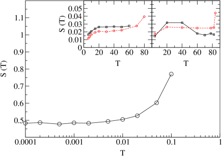
Figure 2: Main panel: Numerical results for the creep rate versus temperature. Details in [5]. Insets: experimental results for the creep rate versus T. The right inset shows data from Keller et al. for melt processed YBCO crystals with the magnetic field applied along the $c$ axis (squares) and $ab$ plane (circles). The left inset shows data from [35] for unirradiated (squares) and 3 MeV proton-irradiated (circles) YBCO flux grown [36] crystals with a 1 T magnetic Field applied parallel to the $c$ axis.

III.3 Biological evolution

In figure 1 we showed that the total population size of the Tangled Nature model, despite of large fluctuations, may also be related to record dynamics. The nature of the metastable states between the quakes is in this case difficult to determine. But we believe they are closely related to the quasi-Evolutionary Stable Strategies which have been identified in the model[30]. We have found that the number of extinctions and creation events per time decreases in the Tangled Nature model[31]. Similar behaviour is observed in macro-evolution[37]. The dynamics of the Tangled Nature model is intermittent as is to some extend clear from Fig. 1. The intermittency is, however, much more evident from analysis of the time dependence of the configurations in genotype, see space[30, 31]. The fossil record has also been interpreted as exhibiting intermittency, see e.g. [38]. Accordingly by comparing the Tangled Nature model and the dynamics of the fossil record we are able to suggest that the decreasing extinction rate and the intermittency, or punctuated equilibrium, is a result a hitherto unrevealed record dynamic that somehow controls the macro-dynamics of biological evolution.

IV Summary and Conclusions

The relevance of record dynamics to the long time evolution of complex systems was indicated by reviewing three very different model studies. The most prominent characteristics of record dynamics are log-Poisson distribution of the number of records, or quakes, occurring during a time interval and a rate of events, which decreases inversely proportional with time. It will be very interesting to analyse the dynamics of other complex systems from the view point of record statistics. The analysis requires access to the time instances at which quakes occur. If that is not available analysis of the probability density function of a single fluctuating quantity such as the heat exchange of a spin glass may suffice to reveal the existence of an underlying record dynamics.

References

- [1] P. Sibani and P.B. Littlewood. Phys. Rev. Lett., 71,1482 (1993).
- [2] P.E. Anderson, H.J. Jensen, L.P. Oliveria, and P. Sibani. Complexity, 10, 49 (2004).
- [3] P. Sibani and H.J. Jensen. JSTAT, P10013 (2004).
- [4] P. Sibani and H.J. Jensen. Europhys. Lett., 69, 563 (2005).
- [5] L.P. Oliveria, H.J. Jensen, and P. Sibani. Phys. Rev. B, in press.
- [6] P. Sibani and A. Pedersen. Europhys. Lett., 48, 346 (1999).
- [7] J. Dall and P. Sibani. Comp. Phys. Comm., 141, 260 (2001).
- [8] J. Dall and P. Sibani. Eur. Phys. J B, 34, 233, (2003).
- [9] P. Sibani and J. Dall. Europhys. Lett., 64,8 (2003).
- [10] S. F. Edwards and P. W. Anderson. J. Phys. F, 5, 965 (1975).
- [11] M. Nicodemi and H.J. Jensen. Physica C, 341-348, 1065 (2000).
- [12] M. Nicodemi and H.J. Jensen. J. Phys. A, 34, L11 (2001).
- [13] M. Nicodemi and H.J. Jensen. Phys. Rev. Lett., 86, 4378 (2001).
- [14] H.J Jensen and M. Nicodemi. Europhys. Lett., 54, 566 (2001).
- [15] M. Nicodemi. Phys. Rev. E, 67, 041103 (2003).
- [16] M. Nicodemi. J. Phys.: Cond Matt., 14, 2403 (2002).
- [17] T. Puig and X. Obradors. Phys. Rev. Lett., 84, 1571 (2000).
- [18] M.F. Goffman et al. Phys. Rev. B, 57, 3663 (1998).
- [19] H. Safar, E. Rodriguez, F. de la Cruz, P. L. Gammel, L. F. Schneemeyer, and D. J. Bishop. Phys. Rev. B, 46, 14238 (1992).
- [20] D. Lopez, G. Nieva, F. de la Cruz, H.J.Jensen, and D. O’Kane. Phys. Rev. B, 50 9684 (1994).
- [21] D. Lopez, E. A. Jagla, E. F. Righi, E. Osquiguil, G. Nieva, E. Morre, F. de la Cruz, and C. A. Balseiro. Physica C, 260, 211 (1996).
- [22] M. B. Gaifullin, Yuji Matsuda, N. Chikumoto, J. Shimoyama, and K. Kishio. Phys. Rev. Lett., 84, 2945 (2000).
- [23] R. Busch, G. Ries, H. Werthner, G. Kreiselmeyer, and G. Saemann-Ischenko. Phys. Rev. Lett., 69, 522 (1992).
- [24] D. T. Fuchs, R. A. Doyle, E. Zeldov, D. Majer, W. S. Seow, R. J. Drost, T. Tamegai, S. Ooi, M. Konczykowski, and P. H. Kes. Phys. Rev. B, 55, R6156 (1997).
- [25] G. Blatter et al. Rev. Mod. Phys., 66, 1199 (1994).
- [26] M. Tinkham. Introduction to Superconductivity. McGraw-Hill, New York, 1996.
- [27] M. Nicodemi and H. J. Jensen. Phys. Rev. B, 65, 144517 (2002).
- [28] D.K. Jacksopn, M. Nicodemi, G.K. Perkins, N.A. Lindop and H.J. Jensen. Europhys. Lett., 52 210 (2000).
- [29] K. Binder. Rep. Prog. Phys., 60, 487 (1997).
- [30] K. Christensen, M. Hall, A. di Collobiano, and H. J. Jensen. J. Theor. Biol., 216, 73 (2002).
- [31] M. Hall, K. Christensen, S.A. di Collabiano, and H.J. Jensen. Phys. Rev. E, 66, 011904 (2002).
- [32] Charles J. Krebs. Ecological Methodology. Benjamin/Cummings, 2nd edition, 1999.
- [33] P. Sibani, C. Schön, P. Salamon, and J.-O. Andersson. Europhys. Lett., 22, 479 (1993).
- [34] C. Darwin. The Origin of Species by Means of Natural Selection. John Murray, more recent edition by Penguing Books 1968, London, 1859.
- [35] L. Civale, A. D. Marwick, M. W. McElfresh, T. K. Worthington, A. P. Malozemoff, F. Holtzberg, J. R. Thompson, and M. A. Kirk. Phys. Rev. Lett., 65, 1164 (1990).
- [36] D.L. Kaiser, F. Holtzberg, M. F. Chisholm, and T. K. Worthington. J. Cryst. Growth, 85, 593 (1987).
- [37] M. E. J. Newman and P. Sibani. Proc. R. Soc. Lond B, 266, 1 (1999).
- [38] N. Eldredge and S. Gould. Nature, 332, 211 (1988).