Current and noise expressions for radio-frequency single-electron transistors

Abstract

We derive self-consistent expressions of current and noise for single-electron transistors driven by time-dependent perturbations. We take into account effects of the electrical environment, higher-order co-tunneling, and time-dependent perturbations under the two-charged state approximation using the Schwinger-Kedysh approach combined with the generating functional technique. For a given generating functional, we derive exact expressions for tunneling currents and noises and present the forms in terms of transport coefficients. It is also shown that in the adiabatic limit our results encompass previous formulas. In order to reveal effects missing in static cases, we apply the derived results to simulate realized radio-frequency single-electron transistor. It is found that photon-assisted tunneling affects largely the performance of the single-electron transistor by enhancing both responses to gate charges and current noises. On various tunneling resistances and frequencies of microwaves, the dependence of the charge sensitivity is also discussed.

I Introduction

For a metallic island small enough to give large charging energy exceeding the temperature, quantum transport through it shows remarkable features due to strongly correlated electrons. A single-electron transistor (SET) is popular geometry of studying transport through the metallic island, in which the island is coupled to two large reservoirs (source and drain) via tunneling junctions and to another reservoir capacitively (gate).houton ; averin ; ingold ; kouwen ; schon The most important principle of operating SET is the Coulomb-blockade effects in the island. In an usual situation particles cannot tunnel into the island due to the Coulomb energy. However, when the Coulomb energy is reduced by a gate bias, transport through the island is possible even with a small bias between the source and drain. Consequently, tunneling currents show a series of peaks, called the Coulomb-blockade peaks, as a function of gate voltage.

From fundamental and applied point of views, the shape of Coulomb-blockade peaks has been attracted much attention and widely studied in static bias conditions.been The appearance of the Coulomb-blockade peaks depends on two conditions. The first is much larger charging energy than the temperature to blockade thermal excitation. The second is thick tunneling barriers guaranteeing a large dwelling time for electrons to resolve the charging energy in the island. Then, from the energy uncertainty principle, the latter is approximately fulfilled under the condition that parallel resistance $R_{T}$ of the barriers is much larger than the resistance quantum $R_{K}=h/e^{2}$, i.e., $\alpha_{0}=R_{K}/(4\pi^{2}R_{T})\ll 1$. It is now well known that for large tunneling resistance $R_{T}$, transport in a SET is achieved by the sequences of uncorrelated tunneling processes and the smearing of peaks is dominated by the temperature. However, for relatively small tunneling resistance ($\alpha_{0}\leq 1$) or very low temperature, additional quantum processes such as higher-order co-tunneling contribute the peaks and renormalizes even its positions as well as associated quantum fluctuation is responsible for the broadening of the peaks.schon ; schoeller It is also found that these higher-order co-tunneling effects are manifested to noises of the system.averin1 ; sukhor ; utsumi On the other hand, in concerning about applications of SETs to an electrometer, a slope of a Coulomb-blockade peak with respect to gate voltages is an important factor. Since the distance between peaks is equal to the change of an elementary charge on the gate, a large slope of the peaks means high sensitivity to a fraction of the charges. So, it is widely believed that a SET is a prime candidate for reading out the final state of a qubit in a solid-state quantum computer.makhlin ; kane ; aassime ; johan

New theoretical interests in transport properties through the strongly correlated systems are emerging together with the experimental success in driving them by microwaves (radio-frequency waves), which are called radio-frequency single-electron transistors (rf SETs).schoel In such a system, microwaves are delivered via a $LC$-resonant circuit to excite particles to overcome the Coulomb energy. As a consequence, SETs can operate in a high-frequency domain and practically provides advantage of a large bandwidth as an electrometer, which allows to measure the rapid variation of gate charges.schoel ; aassime ; fujisawa ; cheong ; buehler Theoretically, the interplay of electronic transport and excitations by microwaves is a particular interest because high-frequency perturbations are expected to yield a new non-equilibrium situation resulted from additional phase variation in energy states.tien Such a time-dependent situation is usually divided into classical and quantum regimes. In the classical regime (or adiabatic regime) energies excited by time-dependent perturbation appear to be continuous while in the quantum regime (we will also refer to this as non-adiabatic regime) discrete photon energies become observable and particles can emit or absorb photons when they tunnel from an initial state on one side of the barrier to a final state on the opposite side, called as photon-assisted tunneling.kouwen1 ; bruder ; staff ; oh

So, in order to understand transport properties of rf SETs, one may need generic theoretical considerations including higher-order co-tunneling processes as well as sequential tunneling, even in the quantum regime of time-dependent perturbations. Actually, according to the recent experiments of rf SETs,aassime ; schoel ; fujisawa ; cheong ; buehler tunneling resistances range from $\alpha_{0}=10^{-5}$ to $3\times 10^{-2}$, implying feasible co-tunneling processes for large values of $\alpha_{0}$. Frequencies of microwaves were used from 0.3 to 1.7 GHz, which correspond to several $\mu eV$ of photon energies, comparable or larger than thermal energy in the experiments. For these values of frequencies, it has been not known for the system to be driven in the classical or quantum regimes of time-dependent perturbations. So, in general it is necessary to solve problems in the quantum regime for more rigorous understanding of transport in rf SETs.

Additionally, tunneling in a rf SET may be dissipative due to a $LC$ resonant circuit. Since a microwave is delivered via a coaxial cable with $50\Omega$ impedance much smaller than the resistance quantum, effects of the electrical environment is usually ignored. This is the case for a $LC$ resonant circuit with a low quality factor, however, with a high-quality factor, energy states of the electrical environment become long-lived because it becomes similar to a simple-harmonic oscillator.devoret ; grabert ; ingold ; schon ; oh1 Then, during tunneling, particles may emit or absorb energy quanta equal to resonant energy of the harmonic oscillator to the environment.

In this work, we develop the formalism that is capable of treating all above theoretical considerations; the effects of higher-order co-tunneling, non-adiabatic time-dependent perturbations, and the electrical environments on operations of rf SETs. Our work is a generalization of several earlier works which address the effects partially, neglecting time-dependent perturbation,utsumi higher-order co-tunneling,bruder ; oh and electron-electron interaction.jauho ; camalet However, since we use a two-charged-state model in a metallic island assuming large charging energy, along this aspect, our work is more restricted than Ref. bruder ; schoeller ; oh . In solving the problem, we use the Schwinger-Keldysh approach combined with a generating functionalutsumi ; negele ; chou ; babi where pseudo-spins of two-charged states are treated with the drone-fermion mapping. Since this approach includes any higher order moment of diagrams systematically, it is one of the well-suited methods for transport through strongly correlated system as indicated in Ref. utsumi . From a generating functional summed diagrammatically, observables of the system are obtained by functional derivatives with respect to external perturbations. This is another advantageous point of this approach because higher-order moments such as noise are easily calculated and expressions for observables are consistent with each other in a sense that they are derived from the same order of diagrams. We express the electrical environment in terms of infinite number of driven harmonic oscillator following Caldeira and Leggetcaldeira where external alternating voltages are treated with classical fields. Based on the unitary transformation which leaves the electrical environment in a stationary situation, we incorporate equilibrium fluctuation of the environment into the generating functional and derive environment- and time-dependent self-energies by counting dominated diagrams. Results for currents and noises are expressed in terms of transport coefficients. In cases of time-dependent perturbations, due to the displacement component currents are found to depend on an additional transport coefficient, leading to a generalization of the Landauer formulalandauer and noises also has its contributions.

The paper is organized as follows. We first describe the model of calculations in Section II. By expressing the dissipative environment in terms of driven harmonic oscillators, we give the Hamiltonian depending on tunneling currents. In Section III, we calculate an approximated generating functional based on the Schwinger-Keldysh approach and discuss several approximations in deriving it. For a given generating functional we show exact expressions for currents and noises in Section IV and rewrite them in terms of transport coefficients. In Section V, we use our formalism to simulate a rf SET numerically and emphasize different points from static calculations. Finally, we summarize our results in Section VI.

II Model of calculations

II.1 Hamiltonian

To formulate the problem of a rf SET, we begin with general circuital geometry of Fig. 1 where time-dependent external sources, $V_{D}(t)$ and $V_{G}(t)$, are supplied via dissipative elements of impedances $Z_{D}(\omega)$ and $Z_{G}(\omega)$.

Figure 1: A typical drawing of the single-electron transistor is shown where time-dependent voltages are applied to a quantum dot via possible dissipative elements connected to drain and gate electrodes, respectively.

In this section we do not specify detailed forms for $Z_{D}(\omega)$ and $Z_{G}(\omega)$ bearing in mind the application of our formalism to other systems concerning effects of dissipative environments.rimberg ; mason ; penttila As a typical model of a SET, a small island is coupled via tunneling barriers to two leads, source and drain, and also capacitively to source, drain, and gates with capacitances of $C_{S}$, $C_{D}$, and $C_{G}$, respectively. We assume that the small island is a metallic one, i.e., there are many energy levels with negligibly small level spacing and also many particles occupied to them. In such a metallic island, one can treat a excess charge of $Q$ confined in it as a independent variable from those of quasiparticles in a good approximation, and usually expresses its Hamiltonian as,bruder ; schoel ; oh ; shnirman

$${\cal H}_{I}=\sum_{nk}\epsilon_{kI}a_{nkI}^{\dagger}a_{nkI}+\frac{Q^{2}}{2C_{\Sigma}}$$ (1)

where $a_{nkI}$($a_{nkI}^{\dagger}$) are the annihilation (creation) operators for quasiparticles with energy $\epsilon_{kI}$ in the island and the index $n$ describes the transverse channels including spin. The second term is a Coulomb-blockade model of the electron-electron interaction with $C_{\Sigma}=C_{D}+C_{S}+C_{G}$. Further simplification of the Coulomb interaction term can be made if one uses a two-state model for excess charges. Assuming the small island enough for charging energy $Q^{2}/2C_{\Sigma}$ to be the largest energy scale in the problem, it is sufficient to consider two number of charged states, say, $\mid 0\rangle$ and $\mid 1\rangle$. Then, the charge operator $Q$ becomes $Q=e\mid\!1\rangle\langle 1\!\mid$ and satisfies $Q^{2}=Q$ (throughout the work $e$ is the proton charge). If we adopt spinor notation, then the Hamiltonian is further written as,

$${\cal H}_{I}=\sum_{nk}\epsilon_{kI}a_{nkI}^{\dagger}a_{nkI}+\Delta_{0}\frac{\sigma_{z}+1}{2}$$ (2)

where $\sigma_{z}$ is the effective spin-1/2 operator and $\Delta_{0}=E_{C}(1-2q_{0}/e)$ is the energy difference between the two charge states together with the charging energy $E_{C}=e^{2}/2C_{\Sigma}$. Here, we anticipate $\Delta_{0}$ which depends on a static component of a gate voltage $V_{G}^{0}$ through a charge of $q_{0}=C_{G}V_{G}^{0}$.

As for the remaining parts of the system, the Hamiltonian can be found by separating it into terms depending on macroscopic and microscopic variables in a similar manner to Ref. oh . Then, the total Hamiltonian may be written as the sum of the unperturbed part and the tunneling part ${\cal H}^{\prime}_{T}$;

$${\cal H}={\cal H}_{I}+{\cal H}_{lead}+{\cal H}_{RLC}(V_{D},V_{G})+{\cal H}^{\prime}_{T}.$$ (3)

Here, ${\cal H}_{I}$, ${\cal H}_{lead}$, and ${\cal H}_{RLC}(V_{D},V_{G})$ represent the unperturbed part of our system, which are shown in Fig. 2. The Hamiltonian ${\cal H}_{lead}=\sum_{nk,\ell=S,D}\epsilon_{k\ell}a_{nk\ell}^{\dagger}a_{nk\ell}$ describes non-interacting electrons in the source and drain with their annihilation ($a_{nk\ell}$) and creation ($a^{\dagger}_{nk\ell})$ operators while the Hamiltonian ${\cal H}_{RLC}(V_{D},V_{G})$ governs the electrical environment which corresponds to a lumped circuit of Fig. 2. Actually, the lumped circuit is designed to exhibit the same dynamical behavior as that of Fig. 1 if it were not for tunneling and thus tunneling barriers work as just capacitances. For this, dynamical variables in the two circuit are related to each other as,

$$\left(\begin{array}[]{c}Q_{1}\\ Q_{2}\\ Q\\ \end{array}\right) = \left(\begin{array}[]{ccc}\frac{C_{1}}{C_{D}}&-\frac{C_{1}}{C_{S}}&0\\ -\frac{C_{2}}{C_{D}}&-\frac{C_{2}}{C_{D}}&\frac{C_{D}}{C_{\Sigma}}\\ -1&-1&-1\\ \end{array}\right)\left(\begin{array}[]{c}Q_{D}\\ Q_{S}\\ Q_{G}\\ \end{array}\right),$$ (13)

$$\left(\begin{array}[]{c}\phi_{D}\\ \phi_{S}\\ \end{array}\right) = {\bf m}\left(\begin{array}[]{c}\phi_{1}\\ \phi_{2}\\ \end{array}\right)=\left(\begin{array}[]{ccc}\frac{C_{1}}{C_{D}}&-\frac{C_{2}}{C_{D}}\\ -\frac{C_{1}}{C_{S}}&-\frac{C_{2}}{C_{D}}\\ \end{array}\right)\left(\begin{array}[]{c}\phi_{1}\\ \phi_{2}\\ \end{array}\right)$$ (22)

where $Q_{\ell}~{}(\ell=D,S,G)$ are excess charges on the capacitors in Fig. 1 and $\phi_{\ell}$ corresponding phases which are related to the potential difference $v_{\ell}(t)$ via the relation of ${\dot{\phi}}_{\ell}(t)=ev_{\ell}(t)/\hbar$. Here, the capacitance $C_{1}$ and $C_{2}$ are defined by $C_{1}=C_{D}C_{S}/(C_{D}+C_{S})$ and $C_{2}=C_{D}^{2}C_{G}/C_{\Sigma}(C_{D}+C_{S})$. Following Caldeira and Leggettcaldeira , one can express the circuit of Fig. 2 in terms of many coupled harmonic oscillators each of which is quantized under the commutation relation of $[\phi_{j},Q_{j}]=ie$. So, considering classical fields of voltage sources applied to the lumped circuit, the electrical environment is described by a set of driven and coupled harmonic oscillators.

Figure 2: Microscopic and macroscopic parts of the single-electron transistor in Fig. 1 are shown. Here, we define $Z_{G}^{\prime}(\omega)=Z_{G}(\omega)(C_{D}+C_{S})^{2}/C_{D}^{2}$ and $V_{G}^{\prime}(t)=V_{G}(t)(C_{D}+C_{S})/C_{D}$.

The tunneling part of the Hamiltonian may be given as,schoeller

$${\cal H}^{\prime}_{T}(t)\! = \!\sum_{\ell=S,D}\sum_{nk,k^{\prime}}\Big{[}T_{kk^{\prime}}^{n\ell}a_{nkI}a_{nk^{\prime}\ell}^{\dagger}\sigma_{+}e^{-i\phi_{\ell}}\!+\!{\rm H.c.}\Big{]}$$ (23)

where $T_{kk^{\prime}}^{n\ell}$ denotes an element of tunneling matrix between a state $\mid\!nk\rangle$ in the lead $\ell$ and a single particle state $\mid\!nk^{\prime}\rangle$ in the island, and usually approximated as $T_{kk^{\prime}}^{n\ell}\simeq T^{\ell}$ independently of energy levels. Here, the operators of $\sigma_{+}$ and $e^{i\phi_{\ell}}$ are inserted for the increase of excess charges in the island and the lead $\ell$, respectively. From the commutation relation the operator $e^{i\phi_{\ell}}$ can be shown to increase excess charges by the elementary charge $e$ in the lead $\ell$ for every tunneling event.

II.2 Current and self-consistent calculations

The current $I_{\ell}(t)$ flowing in each lead of Fig. 1 is defined to be positive if it flows into the island, so that some of charges carrying the current are used to increase charges on the capacitor connected to the lead while the others tunnel into the metallic island. The former represents the displacement current $I^{d}_{\ell}(t)$ which is equal to a time-derivative of the averaged charge as,

$$I^{d}_{\ell}(t)=\frac{d}{dt}\langle Q_{\ell}(t)\rangle_{0}$$ (24)

where $Q_{\ell}(t)$ is the Heisenberg representation of the charge operator $Q_{\ell}$ and $\langle\cdots\rangle_{0}$ stands for the ensemble average. Whereas, the latter is the tunneling current $I^{t}_{\ell}(t)$ which is equal to a time-derivative of the averaged particle number as,

$$I^{t}_{\ell}(t)=e\frac{d}{dt}\langle{\cal N}_{\ell}(t)\rangle_{0}$$ (25)

where ${\cal N}_{\ell}(t)$ is the Heisenberg representation of the number operator ${\cal N}_{\ell}=\sum_{nk}a^{\dagger}_{nk\ell}a_{nk\ell}$ at the lead $\ell$ (we assume particles as electrons). In other words, the current $I_{\ell}(t)$ can be regarded as the sum of the displacement current and the particle current which are contributed from the macroscopic and microscopic system, respectively,

$$I_{\ell}(t)=I^{d}_{\ell}(t)+I^{t}_{\ell}(t)~{}~{}~{}~{}(\ell=D,S,G),$$ (26)

with $I_{G}^{t}=0$. These currents automatically satisfy the current conservation relation of $I_{D}(t)+I_{S}(t)+I_{G}(t)=0$ despite of time-dependent perturbations, as emphasized in Ref. buttiker . This is another consequence of the charge conservation that a Gaussian surface enclosing three capacitors defining the island always contains zero total charges as inferred from Eq. (13). Then, from the continuity equation for charges, the sum of the currents should be zero, alternatively, $d\langle Q(t)\rangle dt=I_{D}^{t}(t)+I_{S}^{t}(t)$ implying the fact that the increase of charges in the island is enabled only by tunneling processes. From the Heisenberg equation of motion for $Q(t)$, one can show that this is the case for our system.

As for the displacement currents, it is possible to obtain further analytic forms because the macroscopic system of ${\cal H}_{RLC}$ consists of linear elements. By viewing the tunneling currents as another external sources as well as voltages of $V_{D}(t)$ and $V_{G}(t)$, from the Heisenberg equations of motion for $Q_{\ell}(t)$ it is straightforward to show that,

$$\left(\begin{array}[]{cc}\frac{1}{i\omega C_{D}}+Z_{D}&-\frac{1}{i\omega C_{S}}\\ -\frac{1}{i\omega C_{G}}-Z_{G}&-\frac{C_{S}+C_{G}}{i\omega C_{S}C_{G}}-Z_{G}\\ \end{array}\right)\left(\begin{array}[]{c}{\tilde{I}}^{d}_{D}(\omega)\\ {\tilde{I}}^{d}_{S}(\omega)\\ \end{array}\right)$$ (31)

$$=\left(\begin{array}[]{c}{\tilde{V}}_{D}(\omega)-{\tilde{V}}_{D}^{t}(\omega)\\ {\tilde{V}}_{G}(\omega)-{\tilde{V}}_{G}^{t}(\omega)\\ \end{array}\right)$$ (34)

where each current is expressed in its Fourier component defined by $I(t)=\int e^{i\omega t}{\tilde{I}}(\omega)d\omega$. Here, the voltages $V_{D}^{t}$ and $V_{G}^{t}$ are given by

$$\left(\begin{array}[]{c}{\tilde{V}}_{D}^{t}(\omega)\\ {\tilde{V}}_{G}^{t}(\omega)\\ \end{array}\right)=\left(\begin{array}[]{cc}Z_{D}&0\\ -\frac{1}{i\omega C_{G}}-Z_{G}&-\frac{1}{i\omega C_{G}}-Z_{G}\\ \end{array}\right)\left(\begin{array}[]{c}{\tilde{I}}^{t}_{D}(\omega)\\ {\tilde{I}}^{t}_{S}(\omega)\\ \end{array}\right)$$ (41)

describing effective voltage lowering by tunneling currents.

With the above expressions for the displacement currents, the problem is now reduced to obtaining the tunneling currents of Eq. (25). For this, it is convenient to transform the system in such a way that the electrical environment of ${\cal H}_{RLC}$ leaves in a stationary condition. Then, under such a situation, harmonic oscillators in ${\cal H}_{RLC}$ are expected to vibrate about their stationary positions. This in turn is helpful to assume them in equilibrium independently of tunneling events even though noises from tunneling may modify their fluctuation slightly. According to Ref. oh , it is possible to find the unitary transformation which rotates the system by voltages of $\delta V_{D}$ and $\delta V_{G}$. By these voltages we mean that the system is rotated to have the lowered voltages in the macroscopic system by the amounts while correspond phases in the tunneling Hamiltonian appear additionally. Namely, the rotated Hamiltonian becomes,

$${\cal H}_{R}\! = \!{\cal H}_{0}+{\cal H}_{T},$$

$${\cal H}_{0}\! = \!{\cal H}_{lead}+{\cal H}_{I}+{\cal H}_{RLC}(V_{D}-\delta V_{D},V_{G}-\delta V_{G}),$$

$${\cal H}_{T}\! = \!\sum_{\ell=D,S}\sum_{nk,k^{\prime}}\Big{[}T^{\ell}a_{nkI}a_{nk^{\prime}\ell}^{\dagger}\sigma_{+}e^{-i\phi_{\ell}-ip_{\ell}(t)}\!+\!{\rm H.c.}\Big{]}.$$ (42)

Here, additional terms of $p_{\ell}(t)(\ell=D,S)$ in the tunneling Hamiltonian actually describe the external phase difference forced by the voltages $\delta V_{D}$ and $\delta V_{G}$ in the absence of tunneling. In other words, it is related to the corresponding potential difference $v_{\ell}^{b}(t)$ across the tunneling barrier from the island to the lead $\ell$ via $p_{\ell}(t)=e/\hbar\int^{t}_{0}d\tau v_{\ell}^{b}(\tau)$. The potential difference $v_{\ell}^{b}(t)$ is given by,

$$\left(\begin{array}[]{cc}\frac{C_{S}+C_{G}}{C_{\Sigma}}&-\frac{C_{D}}{C_{\Sigma}}\\ -\frac{C_{G}}{C_{\Sigma}}&-\frac{C_{G}}{C_{\Sigma}}\\ \end{array}\right){\bf Z}^{-1}\left(\begin{array}[]{c}\tilde{v}^{b}_{D}(\omega)\\ \tilde{v}^{b}_{S}(\omega)\\ \end{array}\right)=\left(\begin{array}[]{c}\frac{\delta{\tilde{V}}_{D}}{Z_{D}}\\ \frac{\delta{\tilde{V}}_{G}}{Z_{G}}\\ \end{array}\right)$$ (49)

where the impedance matrix is defined as,

$${\bf Z}(\omega)\!=\!{\bf m}\left(\begin{array}[]{cc}i\omega C_{1}\!+\!Z_{D}^{-1}\!+\!Z_{G}^{\prime-1}&Z_{G}^{\prime-1}\\ Z_{G}^{\prime-1}&i\omega C_{2}\!+\!Z_{G}^{\prime-1}\\ \end{array}\right)^{-1}\!{\bf m}^{T}$$ (52)

with $Z^{\prime}_{G}=Z_{G}(1+C_{S}/C_{D})^{2}$. Since the number operator ${\cal N}_{\ell}$ is found to be invariant under the rotation, the transformation by $(\delta V_{D},\delta V_{G})=(V_{D}-V_{D}^{t},V_{G}-V_{G}^{t})$ may give rise to the simplest situation in calculating the tunneling currents. In this case, the electrical environment is in stationary conditions as implied from Eq. (41), so that the first moment of its dynamics does not influence the tunneling currents, but the second moment, at least, starts to work.

Instead of this benefit, the rotated Hamiltonian now depends on the tunneling currents. This implies that observables from the Hamiltonian also depends on the tunneling currents unless both $V_{D}^{t}$ and $V_{G}^{t}$ in Eq. (49) are zero. Especially, in cases of the tunneling currents this requires self-consistent calculations to obtain it. Detailed forms in the rotated frame become, from the Heisenberg equation of motion for ${\cal N}_{\ell}$,

$$\begin{array}[]{l}I^{t}_{\ell}(t)=\langle{\cal I}_{\ell}(t)\rangle_{0},\\ {\cal I}_{\ell}(t)={\cal U}^{\dagger}(t,-\infty){\cal J}_{\ell}(t){\cal U}(t,-\infty),\\ {\cal J}_{\ell}(t)=\sum_{nkk^{\prime}}\Big{\{}\frac{e}{i\hbar}T^{\ell}a_{nkI}a_{nk^{\prime}\ell}^{\dagger}\sigma_{+}e^{-i\phi_{\ell}-ip_{\ell}(t)}\!+\!{\rm H.c.}\Big{\}}\end{array}$$ (56)

showing self-consistent behavior. Here, the time-evolution operator ${\cal U}(t,t_{0})$ is defined in the rotated frame as,

$${\cal U}(t,t_{0})={\cal T}\exp\Big{(}\frac{1}{i\hbar}\int_{t_{0}}^{t}d\tau{\cal H}_{R}(\tau)\Big{)},$$ (57)

where ${\cal T}$ is the time-order operator. Once the tunneling currents are calculated self-consistently, other observables depend on them explicitly. For example, current noises are calculated as,

$$S_{\ell\ell^{\prime}}(t,t_{0})=\langle\{\delta{\cal I}_{\ell}(t),\delta{\cal I}_{\ell^{\prime}}(t_{0})\}\rangle_{0}$$ (58)

which is defined by the auto-correlation function of the current fluctuation operator, $\delta{\cal I}_{\ell}(t)={\cal I}_{\ell}(t)-\langle{\cal I}_{\ell}(t)\rangle_{0}$.

II.3 Equilibrium properties of reservoirs

As shown in the unperturbed Hamiltonian, our system consists of three fermionic $({\cal H}_{\ell},\ell=D,S,I)$ and one bosonic $({\cal H}_{RLC})$ systems. We assume these systems as in equilibrium independently of tunneling because, due to large degrees of freedom, effects of tunneling on their fluctuation are expected to be negligible. Then, for the non-interacting fermionic systems, their dynamics are characterized by single-particle Green’s functions. For a $\mid n\rangle$ state with its energy $\epsilon_{n}$ their explicit forms are as follows;

$$g^{K}_{n\ell}(t,t^{\prime})\! \equiv \!\frac{1}{i\hbar}\langle[a_{n\ell}(t),a_{n\ell}^{\dagger}(t^{\prime})]\rangle_{0}$$

$$= \!\frac{1}{i\hbar}{\rm tanh}\frac{\beta\epsilon_{n\ell}}{2}e^{\epsilon_{n\ell}(t-t^{\prime})/i\hbar}$$

$$g^{R}_{n}(t,t^{\prime}) \!\equiv\! \frac{1}{i\hbar}\theta(t\!-\!t^{\prime})\langle\{a_{n}(t),a_{n}^{\dagger}(t^{\prime})\}\rangle_{0}$$

$$= \!\frac{1}{i\hbar}\theta(t\!-\!t^{\prime})e^{\epsilon_{n\ell}(t-t^{\prime})/i\hbar}$$

$$g^{A}_{n}(t,t^{\prime}) \!\equiv\! g^{R*}_{n}(t^{\prime},t)$$ (59)

where $\beta=1/k_{B}T$ is inverse thermal energy and $\epsilon_{n\ell}=\epsilon_{n}-\mu_{\ell}^{0}$ with $\mu_{\ell}^{0}$ an equilibrium chemical potential at a lead $\ell$.chou ; negele ; utsumi

As for the bosonic system of ${\cal H}_{RLC}(V_{D}^{t},V_{G}^{t})$, it is now under a stationary condition; $\langle\phi_{i}(t)\rangle_{0}=\langle Q_{i}(t)\rangle_{0}=0$. Then, its dynamical behavior is characterized by time-correlation functions between variables such as $\langle\phi_{\ell}(0)\phi_{\ell^{\prime}}(t)\rangle_{0}$. In thermal equilibrium, the time-correlation functions are easily evaluated by exploiting the fluctuation-dissipation theorem, and results are,ingold ; oh

$$\langle\phi_{\ell}(0)\phi_{\ell^{\prime}}(t)\rangle_{0}=2\int_{-\infty}^{\infty}\!\frac{d\omega}{\omega}\frac{\Re Z_{\ell\ell^{\prime}}(\omega)}{R_{K}}\frac{e^{i\omega t}}{1-e^{-\hbar\omega\beta}}$$ (60)

where $Z_{\ell\ell^{\prime}}(\omega)$ is related to each component of the impedance matrix ${\bf Z}(\omega)$ in such a way of $Z_{DD}={\bf Z}_{11}$, $Z_{DS}={\bf Z}_{12}$, etc.

III Statistical averages of operators

III.1 Generating functional

To evaluate the ensemble averages for the tunneling currents and noise of Eqs. (56) and (58), we use the Schwinger-Keldysh approach combined with the generating functional technique.utsumi ; chou ; babi We are interested in calculating the expectation value of ${\cal O}$ defined by,

$$\langle{\cal O}(t)\rangle_{0}={\rm Tr}\{\rho_{0}~{}{\cal U}^{\dagger}(t,-\infty)~{}{\cal O}~{}{\cal U}(t,-\infty)\}$$ (61)

where $\rho_{0}$ is the grand canonical density operator describing the system in equilibrium at $t=-\infty$ as,

$$\rho_{0}=\exp\{-\beta({\cal H}_{0}-\sum_{\ell=D,S,I}\mu^{0}_{\ell}{\cal N}_{\ell})\}/Z_{0},$$ (62)

and $Z_{0}$ is the equilibrium partition function. In order to evaluate the expectation value of Eq. (61), we introduce a generating functional $W=-i\hbar~{}{\rm ln}Z$ as an extension of the Gibbs free energy. Here, $Z$ is the generalized partition function defined as,

$$Z={\rm Tr}\{\rho_{0}~{}{\cal U}_{-}^{\dagger}(-\infty,\infty){\cal U}_{+}(\infty,-\infty)\}$$ (63)

where, by different subscripts in the forward ${\cal U}_{+}(\infty,-\infty)$ and backward ${\cal U}^{\dagger}_{-}(-\infty,\infty)$ evolution operators, we mean different external fields applied along each time-branch, respectively. Such different fields are usually coupled to the conjugate variable of ${\cal O}$ in the Hamiltonian and, at the final stage of calculations, are set to be identical. A more compact form of the partition function is obtained if we view the inverse temperature as an imaginary time like,

$$\rho_{0} = \exp\Big{\{}\frac{1}{i\hbar}\int_{-\infty}^{-\infty-i\hbar\beta}d\tau({\cal H}_{0}-\sum_{\ell=D,S,I}\mu_{\ell}{\cal N}_{\ell})\Big{\}}$$ (64)

$$\equiv {\cal U}_{\tau}(-\infty-i\hbar\beta,-\infty).$$

Here, in accordance with Eq. (57), we define this density operator with the evolution operator ${\cal U}_{\tau}$. Then, the partition function becomes,

$$Z = {\rm Tr}\{{\cal U}_{\tau}(-\infty\!-\!i\hbar\beta,-\infty){\cal U}_{-}^{\dagger}(-\infty,\infty){\cal U}_{+}(\infty,-\infty)\}$$ (65)

$$\equiv {\rm Tr}\{{\cal U}_{C}\},$$

and can be interpreted as describing successive evolutions of states along $C_{+}$-, $C_{-}$-, and $C_{\tau}$-time branches as shown in Fig. 3. We designate these time branches simply a closed-time path $C$ bearing in mind that, along each time branch, different Hamiltonians govern the evolution of states; that is, ${\cal H}_{0}+{\cal H}_{T}$ along the $C_{\pm}$-time branches with different fields and ${\cal H}_{0}-\sum_{\ell}\mu_{\ell}{\cal N}_{\ell}$ along the $C_{\tau}$-time branch.

Once the generating functional $W$ is given, the ensemble average of Eq. (61) is obtained through functional derivatives of $W$ with respect to external fields. In cases of the tunneling currents and their noises, the phases $p_{\ell}(t)$ are assumed to be different along each time branch such as,

$$p_{\ell}^{+}(t)\! = \!p_{\ell}(t)\!+\!\frac{\Delta p_{\ell}(t)}{2}~{}~{}~{}~{}{\rm for~{}forward}$$

$$p_{\ell}^{-}(t)\! = \!p_{\ell}(t)\!-\!\frac{\Delta p_{\ell}(t)}{2}~{}~{}~{}~{}{\rm for~{}backward}$$ (66)

where $\Delta p_{\ell}(t)$ is fictitious and will be zero at the final stage. Then, the functional derivatives of the evolution operators with respect to the fictitious field give,

$$\left.\frac{\delta{\cal U}_{+}(\infty,-\infty)}{\delta\Delta p_{\ell}(t)}\right|_{\Delta p_{\ell}\!=\!0}\! = \!\frac{i}{2e}{\cal U}(\infty,t){\cal J}_{\ell}(t){\cal U}(t,-\infty)$$

$$\left.\frac{\delta{\cal U}_{-}^{\dagger}(\infty,-\infty)}{\delta\Delta p_{\ell}(t)}\right|_{\Delta p_{\ell}\!=\!0}\! = \!\frac{i}{2e}{\cal U}(-\infty,t){\cal J}_{\ell}(t){\cal U}(t,\infty)$$ (67)

and, using these relations, it is straightforward to show the tunneling current of Eq. (56) to be,

$$I_{\ell}^{t}(t)=\frac{e}{\hbar}\left.\frac{\delta W}{\delta\Delta p_{\ell}(t)}\right|_{\Delta p_{\ell}=0}.$$ (68)

In a similar way, the current noises are obtained by the second derivatives,

$$S_{\ell\ell^{\prime}}(t,t_{0})\!=\!-\frac{e^{2}}{i\hbar}\Big{\{}\frac{\delta^{2}W}{\delta p_{\ell}^{-}(t)\delta p^{+}_{\ell^{\prime}}(t_{0})}\!+\!\frac{\delta^{2}W}{\delta p_{\ell}^{+}(t)\delta p^{-}_{\ell^{\prime}}(t_{0})}\Big{\}}$$

$$\!=\!\frac{2e^{2}}{i\hbar}\Big{\{}\frac{\delta^{2}W}{\delta\Delta p_{\ell}(t)\delta\Delta p_{\ell^{\prime}}(t_{0})}-\frac{1}{4}\frac{\delta^{2}W}{\delta p_{\ell}(t)\delta p_{\ell^{\prime}}(t_{0})}\Big{\}}$$ (69)

accompanied with $\Delta p_{\ell}(t)=\Delta p_{\ell}(t_{0})=0$ finally. Due to the normalization of the partition function $Z(\Delta p_{\ell}=0)=1$, the second term in the last line of the above equation is equal to zero. Nevertheless, we keep this term to circumvent the uncertainty related to the order of operators.utsumi

Figure 3: Time contour to evaluate the partition function

In order to get the averaged charge in the island and its fluctuation, we add a fictitious field to the excitation energy in such a way of $\Delta_{0}\pm\Delta h(t)/2$. Then, using similar procedure for the tunneling currents, one gets the ensemble average of a charge operator $Q$ as,

$$\langle Q(t)\rangle_{0}=-\left.\frac{e\delta W}{\delta\Delta h(t)}\right|_{\Delta h=0}$$ (70)

while its fluctuation is given by,

$$S_{Q}(t,t_{0})=\langle\{\delta Q(t),\delta Q(t_{0})\}\rangle_{0}~{}~{}~{}~{}~{}~{}~{}~{}~{}~{}~{}~{}~{}~{}~{}~{}~{}~{}~{}~{}~{}~{}~{}~{}~{}~{}~{}~{}~{}~{}$$

$$=2e^{2}\left(\frac{1}{4}\frac{i\hbar\delta^{2}W}{\delta\Delta_{0}(t)\delta\Delta_{0}(t_{0})}-\frac{i\hbar\delta^{2}W}{\delta\Delta h(t)\delta\Delta h(t_{0})}\right)_{\Delta h=0}.$$ (71)

Here, we define the charge fluctuation operators as $\delta Q(t)=Q(t)-\langle Q(t)\rangle_{0}$.

III.2 Evaluation of Generating functional

We evaluate the generating functional $W$ with the coherent-state functional integral method defined on the closed time-path of Fig. 3. As an usual path integral, the evolution operator ${\cal U}_{C}(t)$ is divided into a number of infinitesimal steps on the time-path $C$, and then a resolution of the identity is inserted at every time step. In the coherent state functional integral differently from usual ones, the identity operator is given in terms of eigenfunctions of annihilation operators instead of coordinate- and phase-state basis functions. As a consequence, the evaluation of the partition function $Z$ is reduced to the path integral in coherent-state variables over the exponential of the action along the time contour $C$.negele In our case, the result is summarized as

$$Z=Z_{0}\langle\langle\langle e^{-\frac{1}{i\hbar}S_{int}}\rangle_{{\cal H}_{lead}}\rangle_{{\cal H}_{I}}\rangle_{{\cal H}_{RLC}},$$ (72)

in other words, the exponential of the action $S_{int}$ is averaged over all reservoirs. The action $S_{int}$ describes the interaction among reservoirs, which is given by $S_{int}=\oint_{C}d\tau H_{T}(\tau)$ on the closed time-path $C$. Here, $H_{T}(t)$ is a counterpart of the tunneling Hamiltonian for each time branches, and is obtained by replacing all operators with their coherent-state variables (complex or Grassman numbers) while $H_{T}(t)=0$ in the time branch $C_{\tau}$. As for spins, in order to utilize the coherent-state representation, we map the effective spin-1/2 operators onto two fermion operators $c$ and $d$ (drone-fermion representation), i.e., $\sigma_{+}=c^{\dagger}(d^{\dagger}+d)$ and $\sigma_{z}=2c^{\dagger}c-1$.utsumi

By the bracket notation, we mean an average weighted with the action of a certain reservoir. The detailed form is defined, for instance over ${\cal H}_{lead}$, as

$$\langle O\rangle_{{\cal H}_{lead}}=\frac{1}{Z_{0}^{lead}}\int{\cal D}[a_{rk\ell}(t),a^{*}_{rk\ell}(t)]e^{-\frac{1}{i\hbar}S_{lead}}~{}O$$ (73)

where $Z_{0}^{lead}$ is a normalization factor implying $\langle 1\rangle_{{\cal H}_{lead}}=1$ and equal to the equilibrium partition function of ${\cal H}_{lead}$. Here, $\{a_{nk\ell}(t),a_{nk\ell}^{*}(t)\}$ are Grassmann variables associated with their fermionic operators and they satisfy anti-periodic boundary conditions; $a_{nk\ell}(-\infty\in C_{+})=-a_{nk\ell}(-\infty-i\hbar\beta\in C_{\tau})$. The unperturbed action of the leads $S_{lead}$ is given as,

$$S_{lead}=i\hbar\oint_{C}d\tau\Big{\{}\sum_{nk\ell}a^{*}_{nk\ell}(\tau)\frac{\partial}{\partial\tau}a_{kn\ell}(\tau)\!-\!H_{lead}(\tau)\Big{\}}$$ (74)

using the trajectory notation, in which the function $H_{lead}(t)$ represents ${\cal H}_{lead}$ and ${\cal H}_{lead}-\sum_{\ell}\mu_{\ell}{\cal N}_{\ell}$ in the time branches $C_{\pm}$ and $C_{\tau}$ respectively.

Since the unperturbed actions are quadratic, the thermal average over all reservoirs of Eq. (72) is reduced to Gaussian times polynomial integrals if one expands $e^{-S_{int}/i\hbar}$ into a power series. Then, using a standard procedure of a Gaussian integral, each term in the series can be evaluated analytically. Firstly the result over the reservoirs $(\ell=D,S,I)$ is summarized by the appearance of a particle-hole Green’s function $b_{\ell}(t,t^{\prime})$ in the action $S_{int}$. The Green’s function $b_{\ell}(t,t^{\prime})$ has a form of,

$$b_{\ell}(t,t_{0}) = -i\hbar N_{ch}\sum_{k}\mid T^{\ell}\mid^{2}g_{kI}(t,t_{0})g_{k\ell}(t_{0},t)$$ (75)

$$e^{ip_{\ell}(t)-ip_{\ell}(t_{0})},~{}~{}~{}~{}~{}\ell=D,S$$

Here, the free-particle Green’s functions $g_{k\ell}(t,t_{0})$ represents the inverse function of their free actions and their physical representations are equal to Eq. (59) which can be obtained by the Keldysh rotation. Then, the function $b_{\ell}(t,t^{\prime})$ represents just a single particle or hole creation in the island by tunneling through a barrier $\ell$. Actually, in obtaining $b_{\ell}(t,t^{\prime})$ we take into account only sequential processes of single particle or hole creation; one can see it if expanding the exponential of $S_{int}$ into a series. This is a good approximation for a large number of transverse channels $N_{ch}$, so called, the wide junction limit because the sequential particle or hole creation is dominated to the simultaneous creation of both, at least, by $N_{ch}$.schoeller

These sequential processes are correlated by further evaluation of the partition function over the $c-$ and $d-$ fields. The result reads,

$$Z=Z_{0}\left\langle\exp\Big{[}-\sum_{n=1}\frac{1}{n}{\rm Tr}\{(g_{c}\frac{\delta}{\delta\eta}B\frac{\delta}{\delta\eta})^{n}\}\Big{]}\right\rangle_{{\cal H}_{RLC}}$$

$$\left.\exp\{-i\hbar\int_{C}dtdt_{0}~{}\eta(t)g_{d}(t,t_{0})\eta(t_{0})\}\right|_{\eta=0}$$ (76)

where the simplified notation of ${\rm Tr}\{g_{c}\frac{\delta}{\delta\eta}B\frac{\delta}{\delta\eta}\}$ stands for

$${\rm Tr}\{g_{c}\frac{\delta}{\delta\eta}B\frac{\delta}{\delta\eta}\}\!=\!\int_{C}\!dt\!dt_{0}g_{c}(t,t_{0})\frac{\delta}{\delta\eta(t_{0})}B(t_{0},t)\frac{\delta}{\delta\eta(t)}$$ (77)

and $B$ is the particle-hole Green’s function combined with effects of the electrical environment by

$$B(t,t_{0})=\sum_{\ell}e^{-i\phi_{\ell}(t)}b_{\ell}(t,t_{0})e^{i\phi_{\ell}(t_{0})}.$$ (78)

Here, $g_{c}$ and $g_{d}$ are equilibrium Green’s functions for the $c-$ and $d-$ fields with their eigenenergies $\Delta_{0}$ and zero, respectively. The Grassmann field $\eta(t)$ is introduced as a linear source to the $d$-field, which gives an additional term of $-i\hbar\int_{C}dt[\eta(t)d(t)-d^{*}(t)\eta(t)]$ into the unperturbed action.

Finally, we evaluate the partition function over the electrical environment. To do this, we transform bi-linearly coupled harmonic oscillators in ${\cal H}_{RLC}$ into independent ones by an unitary transformation. Then, since each simple harmonic oscillator is assumed to be in equilibrium, one can exploit the Wick’s theorem to show that its thermal average can be expressed in terms of, at most, the second order phase correlation. To each term of the series in Eq. (76), the application of the theorem leads to the relation of,

$$\langle e^{i\phi_{\ell_{1}}(1)}e^{-i\phi_{\ell_{2}}(2)}\ldots e^{-i\phi_{\ell_{n}}(n)}\rangle_{{\cal H}_{RLC}}=$$

$$e^{K_{\ell_{1}\ell_{2}\ldots\ell_{n}}(1,2,\ldots,n)}$$ (79)

where $K_{\ell_{1}\ell_{2}\ldots}(1,2,\ldots,n)$ is defined by

$$K_{\ell_{1}\ell_{2}\ldots\ell_{n}}(1,2,\ldots,n)=~{}~{}~{}~{}~{}~{}~{}~{}~{}~{}~{}~{}~{}~{}~{}~{}~{}~{}~{}~{}~{}~{}~{}~{}~{}$$

$$\frac{1}{2}\langle[i\phi_{\ell_{1}}(1)\!-\!i\phi_{\ell_{2}}(2)\!+\ldots-i\phi_{\ell_{n}}(n)]^{2}\rangle_{{\cal H}_{RLC}}.$$ (80)

According to this, $K_{\ell_{1}\ell_{2}\ldots}(1,2,\ldots)$ is the sum of the second-order correlation functions among all time-arguments, so that all sequential processes of microscopic variables in each term of Eq. (76) are correlated additionally. Actually, the second-order correlation function of $\langle\phi_{\ell}(1)\phi_{\ell^{\prime}}(2)\rangle_{{\cal H}_{RLC}}$ is related to the phase fluctuations of Eq. (60). One of simple ways for this is to display the fluctuation-dissipation theorem in terms of $K_{\ell_{1}\ell_{2}}(1,2)$ and then, by comparing it with Eq. (60), one obtains;

$$\langle\phi_{\ell}(t)\phi_{\ell^{\prime}}(t_{0})\rangle_{{\cal H}_{RLC}}^{-+} = \langle\phi_{\ell}(t)\phi_{\ell^{\prime}}(t_{0})\rangle_{0}$$

$$\langle\phi_{\ell}(t)\phi_{\ell^{\prime}}(t_{0})\rangle_{{\cal H}_{RLC}}^{+-} = \langle\phi_{\ell}(t)\phi_{\ell^{\prime}}(t_{0})\rangle_{0}^{*}$$

$$\langle\phi_{\ell}(t)\phi_{\ell^{\prime}}(t_{0})\rangle_{{\cal H}_{RLC}}^{++} = \theta(t-t_{0})\langle\phi_{\ell}(t)\phi_{\ell^{\prime}}(t_{0})\rangle_{0}$$

$$+ \theta(t_{0}-t)\langle\phi_{\ell}(t)\phi_{\ell^{\prime}}(t_{0})\rangle_{0}^{*}$$

$$\langle\phi_{\ell}(t)\phi_{\ell^{\prime}}(t_{0})\rangle_{{\cal H}_{RLC}}^{--} = \theta(t-t_{0})\langle\phi_{\ell}(t)\phi_{\ell^{\prime}}(t_{0})\rangle_{0}^{*}$$ (81)

$$+ \theta(t_{0}-t)\langle\phi_{\ell}(t)\phi_{\ell^{\prime}}(t_{0})\rangle_{0}$$

where superscripts of $\pm\!\mp$ denote each section of the Keldysh space in which both time arguments $t$ and $t_{0}$ belong.

The generating functional $W$ is now calculated by summing all-connected diagrams in $Z$. To prevent the divergence of the average charge at $\Delta_{0}=0$, we perform diagrammatic sum to infinite order, however approximated forms in higher-order diagrams cannot be inevitable for a simple form of $W$. Expanding the partition function of Eq. (76) and arranging diagrams, we write the approximated generating functional as,

$$W \simeq -i\hbar\left({\rm Tr}[{\rm ln}g_{c}^{-1}]-{\rm Tr}[g_{c}\Sigma^{(1)}]-\frac{1}{2}{\rm Tr}[g_{c}\Sigma^{(2)}]\right.$$ (82)

$$\left.-\frac{1}{3}{\rm Tr}[g_{c}\Sigma^{(3)}]+\cdots\right)$$

where we omit trivial non-interacting terms. In the first-order term, a single diagram contributes the generating functional and its self-energy has a form of,

$$\Sigma^{(1)}(t,t_{0}) = \sum_{\ell}e^{K_{\ell\ell}(t,t_{0})}\Sigma^{f}_{\ell}(t,t_{0})$$ (83)

with a free-environment part of,

$$\Sigma^{f}_{\ell}(t,t_{0})=-2i\hbar g_{d}(t_{0},t)b_{\ell}(t,t_{0}).$$ (84)

However, for each higher-order term from the second, rich connected diagrams are found. We approximate the generating function by taking into account only a single diagram in each $n$_order with its self energies of,

$$\Sigma^{(n)}(t,t_{0})=\sum_{\ell_{1}..\ell_{n}}\int_{C}d1d2..dne^{K_{\ell_{1}\ell_{1}\ldots\ell_{n}\ell_{n}}(t,1,2,..,t_{0})}$$

$$\Sigma^{f}_{\ell_{1}}(t,1)g_{c}(1,2)\Sigma^{f}_{\ell_{2}}(2,3)g_{c}(3,4)..\Sigma^{f}_{\ell_{n}}(n,t_{0}).$$ (85)

The idea for such preferred diagrams comes from the work of Utsmi et. al.utsumi Actually, the partition function of $Z$ is the same as that in their work if it were not for the electrical environment and time-dependent perturbations. So we compose the approximated generating functional to recover their results in the absence of the electrical environment and time-dependent perturbations, say, in the case of $K_{\ell\ldots}=0$ and $p_{\ell}(t)=0$.

As a result, the generating functional can be written in a more compact form as,

$$W = -i\hbar\left({\rm Tr}[{\rm ln}g_{c}^{-1}]-\sum_{n=1}^{\infty}\frac{1}{n}{\rm Tr}[(g_{c}\Sigma)^{n}]\right)$$ (86)

$$= -i\hbar~{}{\rm Tr}[{\rm ln}G^{-1}]$$

where we introduce the full $c$-field Green’s function $G$ obeying the Dyson equation;

$$G^{-1}(t,t_{0})=g_{c}^{-1}(t,t_{0})-\Xi(t,t_{0})$$ (87)

with a noninteracting Green’s function $g_{c}(t,t_{0})$ of the $c-$ field. Here, the self-energy $\Xi(t,t_{0})$ is defined by,

$$\Xi(t,t_{0})=\Sigma^{(1)}(t,t_{0})$$

$$+\frac{1}{2}\left[\Sigma^{(2)}-\Sigma^{(1)}g_{c}\Sigma^{(1)}\right](t,t_{0})$$

$$+\frac{1}{3}\left[\Sigma^{(3)}-\frac{3}{2}\Sigma^{(2)}g_{c}\Sigma^{(1)}+\frac{1}{2}\Sigma^{(1)}g_{c}\Sigma^{(1)}g_{c}\Sigma^{(1)}\right](t,t_{0})$$

$$+\ldots$$

$$\simeq\Sigma^{(1)}(t,t_{0})$$ (88)

which is obtained by comparing Eqs. (82) and (86). Since Eq. (87) already sum up an infinite series, we calculate $\Xi(t,t_{0})$ to the lowest order of $\Sigma^{(1)}(t,t_{0})$. This is equivalent to neglecting additional correlations caused by the electrical environment in higher-order terms of the above equation. In this case, the self-energy of $\Xi(t,t_{0})$ is expressed explicitly with the product of terms representing effects of time-dependent perturbations and the electrical environment, respectively, as

$$\Xi(t,t_{0}) = \Xi_{D}(t,t_{0})+\Xi_{S}(t,t_{0}),$$

$$\Xi_{\ell}(t,t_{0}) = e^{ip_{\ell}(t)}\Sigma_{\ell}(t,t_{0})e^{-ip_{\ell}(t_{0})},$$

$$\Sigma_{\ell}(t,t_{0}) = e^{K_{\ell\ell}(t,t_{0})}\Sigma^{0}_{\ell}(t,t_{0})$$ (89)

and thus $\Sigma^{0}_{\ell}$ represents the free self-energy from the environment and time-dependent perturbations,

$$\Sigma^{0}_{\ell}(t,t_{0}) = -2\hbar^{2}N_{ch}g_{d}(t_{0},t)\mid T^{\ell}\mid^{2}$$ (90)

$$\sum_{k}g_{kI}(t,t_{0})g_{k\ell}(t_{0},t).$$

IV Expressions for currents and noises

For the given generating functional and the self-energy of Eqs. (86) and (89), we now derive exact expressions for tunneling currents, averaged charges, and their noises. Using the standard procedure, we perform functional derivatives as specified in Eqs. (68), (69), (70), and (71), and transform them into the physical representation. The transformations are carried out by adopting the Keldysh rotator as, for instance of $G$,

$$\left(\begin{array}[]{cc}G^{+\!+}&G^{+\!-}\\ G^{-\!+}&G^{-\!-}\end{array}\right)\!=\!\frac{1}{2}\left(\begin{array}[]{cc}1&1\\ -\!1&1\end{array}\right)\left(\begin{array}[]{cc}0&G^{A}\\ G^{R}&G^{K}\end{array}\right)\left(\begin{array}[]{cc}1&-\!1\\ 1&1\\ \end{array}\right),$$ (99)

where superscripts $A$, $R$, and $K$ denote its advanced, retarded, and Keldysh components, respectively.

Then, with this rotator the Dyson equation of Eq. (87) is transformed as;

$$G^{R}(t,t_{0})=g_{c}^{R}(t,t_{0})~{}~{}~{}~{}~{}~{}~{}~{}~{}~{}~{}~{}~{}~{}~{}~{}~{}~{}~{}~{}~{}~{}~{}~{}~{}~{}~{}~{}~{}~{}~{}~{}~{}~{}~{}~{}~{}~{}~{}~{}$$

$$+\int_{-\infty}^{\infty}d\tau_{1}d\tau_{2}g_{c}^{R}(t,\tau_{1})\Xi^{R}(\tau_{1},\tau_{2})G^{R}(\tau_{2},t_{0})$$

$$G^{K}(t,t_{0})\!=\!\int_{-\infty}^{\infty}\!d\tau_{1}\!d\tau_{2}G^{R}(t,\!\tau_{1})\Xi^{K}(\tau_{1},\!\tau_{2})G^{A}(\tau_{2},\!t_{0})$$

$$G^{A}(t,t_{0})\!=\!G^{R*}(t_{0},t)~{}~{}~{}~{}~{}~{}~{}~{}~{}~{}~{}~{}~{}~{}~{}~{}~{}~{}~{}~{}~{}~{}~{}~{}~{}~{}~{}~{}~{}~{}~{}~{}~{}~{}~{}~{}~{}~{}$$ (100)

where $g_{c}^{R}(t,t_{0})$ is a retarded component of the free-particle Green’s function specified in Eq. (59). According to these relations, $G^{R,A}$ has the same causality relation as that of $g_{c}^{R,A}$, and additionally satisfies the sum rule of $\lim_{t\rightarrow t_{0}}i\hbar G^{C}(t,t_{0})=1$ with $G^{C}\equiv G^{R}-G^{A}$. For $G^{K}$, we show it in terms of $G^{R}$ and $G^{A}$ rather than its integral equation by noting that $({\bf 1}+G^{R}\Sigma^{R})g_{c}^{K}=G^{R}(g_{c}^{R})^{-1}g_{c}^{K}$ vanishes. On the other hand, the application of the rotator to the self-energy of Eq. (89) leads to

$$\begin{array}[]{l}\Sigma^{R}_{\ell}(t,t_{0})=\Sigma^{0R}_{\ell}(t\!-\!t_{0})\Re e^{K^{-+}_{\ell\ell}(t,t_{0})}\\ ~{}~{}~{}~{}~{}~{}~{}~{}~{}~{}~{}+i\Sigma^{0K}_{\ell}(t\!-\!t_{0})\Im e^{K^{-+}_{\ell\ell}(t,t_{0})}\theta(t\!-\!t_{0}),\\ \Sigma^{K}_{\ell}(t,t_{0})=\Sigma^{0K}_{\ell}(t\!-\!t_{0})\Re e^{K^{-+}_{\ell\ell}(t,t_{0})}\\ ~{}~{}~{}~{}~{}~{}~{}~{}~{}~{}~{}+i\Sigma^{0C}_{\ell}(t\!-\!t_{0})\Im e^{K^{-+}_{\ell\ell}(t,t_{0})},\\ \Sigma^{A}_{\ell}(t,t_{0})=\Sigma^{R}_{\ell}(t_{0},t)^{*}.\end{array}$$ (106)

Here, we arrange each term to depend only on the correlation function of $K^{-+}_{\ell\ell}(t,t_{0})$. Thus, the self-energy of $\Sigma_{\ell}$ is directly related to the phase fluctuation of Eq. (60) via $K^{-+}_{\ell\ell}(t,t_{0})=\langle\phi_{\ell}(0)[\phi_{\ell}(t_{0}-t)-\phi_{\ell}(0)]\rangle_{0}$.

A detailed form of the bare self-energy $\Sigma^{0}_{\ell}$ depends on a cut-off function for the spectral density of the particle-hole propagator $b_{\ell}$. In this work we use a Lorenzian cut-off function $\rho(E)=EE_{0}^{2}/(E^{2}+E_{0}^{2})$ with a bandwidth of $E_{0}=E_{C}$ as in earlier works.schoeller ; utsumi Then, by substituting free-particle Green’s functions and $\rho(E)$ into (90), and transforming into Fourier forms by

$$\Sigma^{0}_{\ell}(t,t_{0})=\frac{1}{2\pi}\int d\omega e^{-i\omega(t-t_{0})}\tilde{\Sigma}^{0}_{\ell}(\hbar\omega),$$ (107)

we find,

$$\tilde{\Sigma}^{0R}_{\ell}(\epsilon) = \frac{R_{K}}{4\pi^{2}R_{\ell}}\rho(\epsilon_{\ell})\Big{[}2\Re~{}\psi_{0}(1\!+\!i\frac{\epsilon_{\ell}\beta}{2\pi})$$

$$- \psi_{0}(1\!+\!\frac{E_{0}\beta}{2\pi})-\psi_{0}(\frac{E_{0}\beta}{2\pi})\!-\!i\pi{\rm coth}\frac{\beta\epsilon_{\ell}}{2}\Big{]},$$

$$\tilde{\Sigma}^{0K}_{\ell}(\epsilon) = i\frac{R_{K}}{2\pi R_{\ell}}\rho(\epsilon_{\ell}),$$

$$\tilde{\Sigma}^{0A}_{\ell}(\epsilon) = \tilde{\Sigma}^{0R*}_{\ell}(\epsilon)$$ (108)

where $\epsilon_{\ell}=\epsilon-\mu_{\ell}^{0}$ and $\psi_{0}$ is a digamma function. Here, $R_{\ell}$ stands for $1/R_{\ell}=4\pi^{2}N_{ch}\mid\!T^{\ell}\!\mid^{2}D_{I}D_{\ell}/R_{K}$ with energy-independent density of states $D_{I}$ and $D_{\ell}$ at the metallic island and the lead $\ell$, respectively. This is tunneling resistance of the barrier connected to the lead $\ell$, so that the parallel resistance is given by $1/R_{T}=1/R_{D}+1/R_{S}$ in $\alpha_{0}=R_{K}/(4\pi^{2}R_{T})$.

For static conditions, an analytical solution of the Dyson equation in Eq. (100) is easily obtained by transforming it to the Fourier space. However, for arbitrary time-dependent perturbation since the time-translational invariance of the self-energy is broken, the solution shows up in a series or it is necessary to solve the problem numerically. One of approximated solutions may be derived by noting that $\Sigma^{0}_{\ell}(t,t_{0})$ exhibits rapid decaying behavior as a function of time interval $t-t_{0}$. If this is the fastest time-variation in the problem, the integral equation can be approximated to the first-order differential equation. Then, the solution becomes similar to that obtained in the the wide-band limit.jauho

With the physical representation of the Green’s functions and the self-energies, results of the functional derivatives are summarized as the followings. The averaged charge in the island and the tunneling currents are given as,

$$\langle Q(t)\rangle_{0}\! = \!-e\frac{i\hbar}{2}G^{K}(t,t),$$ (109)

$$I_{\ell}^{t}(t)\! = \!-e\Re\Gamma_{\ell}^{K}(t,t)$$ (110)

while their fluctuations read

$$S_{Q}(t,t_{0}) = \frac{\hbar^{2}e^{2}}{2}G^{K}(t,t_{0})G^{K}(t_{0},t)-(K\rightarrow C),$$ (111)

$$S_{\ell\ell^{\prime}}(t,t_{0}) = e^{2}\Re\Big{\{}\Xi^{K}_{\ell}(t,t_{0})G^{K}(t_{0},t)\delta_{\ell\ell^{\prime}}$$ (112)

$$+ \!\Lambda_{\ell\ell^{\prime}}^{K}(t,t_{0})G^{K}(t_{0},t)-\Gamma^{K}_{\ell}(t,t_{0})\Gamma_{\ell^{\prime}}^{K}(t_{0},t)\Big{\}}$$

$$- (K\rightarrow C)$$

where $(K\rightarrow C)$ means the change of a Keldysh component to a correlated one, for example, $G^{K}\rightarrow G^{C}=G^{R}-G^{A}$. Here, the functions of $\Gamma$ and $\Lambda$ are defined as,

$$\Gamma_{\ell}^{K,C}(t,t_{0}) = \int_{-\infty}^{\infty}d\tau\Big{[}\Xi^{K,C}_{\ell}(t,\tau)G^{A}(\tau,t_{0})$$

$$+ \Xi^{R}_{\ell}(t,\tau)G^{K,C}(\tau,t_{0})\Big{]},$$

$$\Lambda_{\ell\ell^{\prime}}^{K,C}(t,t_{0}) = \int_{-\infty}^{\infty}d\tau\Big{[}\Gamma^{K,C}_{\ell}(t,\tau)\Xi_{\ell^{\prime}}^{A}(\tau,t_{0})$$ (113)

$$+ \Gamma^{R}_{\ell}(t,\tau)\Xi_{\ell^{\prime}}^{K,C}(\tau,t_{0})\Big{]},$$

with $\Xi^{C}_{\ell}=\Xi^{R}_{\ell}-\Xi^{A}_{\ell}$. With these fluctuations, the noise spectrum at a frequency $\omega$ is defined by,davies ; hanke ; korotkov

$$S_{Q}(\omega) = \langle\!\langle S_{Q}(t,t_{0})\cos\omega(t-t_{0})\rangle\!\rangle$$

$$S_{\ell\ell^{\prime}}(\omega) = \langle\!\langle S_{\ell\ell^{\prime}}(t,t_{0})\cos\omega(t-t_{0})\rangle\!\rangle$$ (114)

where the double bracket denotes the integration of,

$$\langle\!\langle...\rangle\!\rangle=\Re\left[\lim_{T\rightarrow\infty}\frac{1}{T}\int_{0}^{T}dt_{0}\int_{-\infty}^{\infty}dt~{}...\right].$$ (115)

As discussed in the previous section the above results obey the charge conservation law even under arbitrary time-dependent perturbations, i.e.

$$\frac{\partial\langle Q(t)\rangle_{0}}{\partial t} = \sum_{\ell}I_{\ell}^{t}(t),$$ (116)

$$\frac{\partial^{2}S_{Q}(t,t^{\prime})}{\partial t\partial t^{\prime}} = \sum_{\ell\ell^{\prime}}S_{\ell\ell^{\prime}}(t,t^{\prime}).$$ (117)

This is also a direct consequence of the guage-invariant generating functional of Eq. (86).

The equations of Eq. (109)-(112) are the main results of our work together with the generalized self-energies of Eq. (89) to arbitrary time-dependent perturbations and electrical environments. Even though the above equations give the exact expressions within the given generating functional and provide easier ways in numerical calculations, their physical meanings are not well revealed. So, in the subsequent section we present another forms by considering various limits.

IV.1 Wide-band limit

In order to obtain more physically meaningful forms we start with defining a spectral function $A_{\ell}(\epsilon,t)$ as

$$A_{\ell}(\epsilon,t)=\int_{-\infty}^{\infty}d\tau e^{i\epsilon(\tau-t)/\hbar}e^{-ip_{\ell}(\tau)}G^{A}(\tau,t)$$ (118)

and writing ${\tilde{\Sigma}}^{K}_{\ell}(\epsilon)$ as,

$$\tilde{\Sigma}^{K}_{\ell}(\epsilon)=\tilde{\Sigma}_{\ell}^{C}(\epsilon)\{2f_{\ell}(\epsilon)-1\}$$ (119)

where $f_{\ell}(\epsilon)$ is a Fermi-Dirac distribution function broadened due to the presence of the dissipative environment, otherwise, it is equal to $f_{\ell}(\epsilon)=1/(1+e^{\beta(\epsilon-\mu_{\ell}^{0})})$. Then, from Eq. (109) the average charge can be rewritten as,

$$\langle Q(t)\rangle_{0} = e\sum_{\ell}\int d\epsilon~{}n_{\ell}(t,t;\epsilon)\{f^{+}_{\ell}(\epsilon)-f_{\ell}(\epsilon)\}$$ (120)

where, by defining a hole-distribution function, $f^{+}_{\ell}(\epsilon)=1-f_{\ell}(\epsilon)$, we emphasize the roles of hole and electron contributions. Here, $n_{\ell}(t,t;\epsilon)$ is a diagonal value of,

$$n_{\ell}(t,t_{0};\epsilon)\equiv\frac{i}{4\pi}e^{-i\epsilon(t-t_{0})/\hbar}{\tilde{\Sigma}}_{\ell}^{C}(\epsilon)A_{\ell}^{*}(\epsilon,t)A_{\ell}(\epsilon;t_{0}),$$ (121)

which can be interpreted as, owing to its unit, the evolution of density of states at the lead $\ell$ available to occupying the island.

As for the tunneling currents, we additionally exploit the relation of $(1+\Xi^{R}G^{R})=(i\hbar\partial_{t}-\Delta_{0})G^{R}$ and then obtain the form of, from Eq. (110),

$$I_{\ell}^{t}(t)=\frac{1}{2eR_{K}}\Re\!\int_{-\infty}^{\infty}d\epsilon\Big{[}~{}~{}~{}~{}~{}~{}~{}~{}~{}~{}~{}~{}~{}~{}~{}~{}~{}~{}~{}~{}~{}~{}~{}~{}~{}~{}~{}~{}~{}~{}~{}~{}~{}$$

$$\left\{T^{F}_{\ell}(t,t;\epsilon)\!-\!T^{R}_{\ell}(t,t;\epsilon)\right\}\left\{f^{+}_{\ell}(\epsilon)\!-\!f_{\ell}(\epsilon)\right\}$$

$$-T^{F}_{\bar{\ell}}(t,t;\epsilon)\left\{f^{+}_{\bar{\ell}}(\epsilon)\!-\!f_{\bar{\ell}}(\epsilon)\right\}\Big{]}$$ (122)

where the first term in the right-hand side represents the particle flux from the lead $\ell$ and the second is the flux from the opposite-side lead ${\bar{\ell}}$. Here, $T^{F}_{\ell}(t,t;\epsilon)$ and $T^{R}_{\ell}(t,t;\epsilon)$ are transport coefficients representing tunneling of holes (electrons) in the region of positive (negative) energies. The function $T^{F}_{\ell}(t,t;\epsilon)$ is a diagonal part of,

$$T^{F}_{\ell}(t,t_{0};\epsilon) = 4\pi i\int_{-\infty}^{\infty}d\tau e^{ip_{\ell}(t)}\Sigma_{\bar{\ell}}^{C}(t,\tau)e^{-ip_{\ell}(\tau)}$$ (123)

$$n_{\ell}(\tau,t_{0};\epsilon)$$

which depends on both sides of the tunneling barriers and can be considered as the transmission function from the lead $\ell$ to the other side ${\bar{\ell}}$. In writing $T_{\ell}^{F}$, we adopt an approximated form for its further use by substituting $\Sigma_{\bar{\ell}}^{C}$ instead of $2\Sigma^{R}_{\bar{\ell}}$. This approximation corresponds to the wide-band limit.jauho With this transmission function alone, the expression of Eq. (122) is consistent with the well-known Laudauer formula.landauer However, the additional function $T^{R}_{\ell}$ gives rise to a deviated form from the formula; $T^{R}_{\ell}$ is given by,

$$T^{R}_{\ell}(t,t_{0};\epsilon) = \!8\pi i\left(i\hbar\frac{\partial}{\partial t}-\Delta_{0}\right)n_{\ell}(t,t_{0};\epsilon).$$ (124)

According to this, $T^{R}_{\ell}(t,t_{0};\epsilon)$ is independent of the other-side tunneling barrier $\bar{\ell}$ contrast to $T^{F}_{\ell}$ implying not a transmission function and, moreover, it does not appear in the flux from the other-side lead ${\bar{\ell}}$. These facts are likely to interpret the function as a transport coefficient describing the electron or hole flux supplied by the metallic island. This becomes more apparent if one compares $T^{R}_{\ell}$ with Eq. (120) where the flux by $T^{R}_{\ell}$ is equal to the decrease rate of charges in the island. This flux has no a stationary component to be $\Re T^{R}_{\ell}(t,t;\epsilon)=0$, by which our expression successfully recovers the Landauer formula in a static condition.

On the other hand, the charge noise is rearranged to be,

$$S_{Q}(t,t_{0})\! = \!\sum_{\ell\ell^{\prime}}S_{Q}^{\ell\ell^{\prime}}(t,t_{0})$$

$$S_{Q}^{\ell\ell^{\prime}}(t,t_{0})\! = \!4e^{2}\int_{-\infty}^{\infty}\!d\epsilon_{1}\!d\epsilon_{2}~{}n_{\ell}(t,t_{0};\epsilon_{1})n_{\ell^{\prime}}(t_{0},t;\epsilon_{2})$$ (125)

$$\left\{f_{\ell}(\epsilon_{1})f_{{\bar{\ell}}}^{+}(\epsilon_{2})+f_{\ell}^{+}(\epsilon_{1})f_{{\bar{\ell}}}(\epsilon_{2})\right\},$$

which is the sum of all possible electron-hole correlations tunneled from both leads.

The current noise in time-dependent cases is found to have a complicated form due to the fluctuations arising from various origins and, therefore, we show it under the wide-band approximation separating into three contributions. The self correlation of the tunneling current at the lead $\ell$ is arranged as,

$$S_{\ell\ell}(t,t_{0})=S_{v}^{\ell}(t,t_{0})+S_{r}^{\ell}(t,t_{0})+\frac{\partial^{2}}{\partial t\partial t_{0}}S_{Q}^{\ell\ell}(t,t_{0})$$ (126)

while the correlation between the different-side tunneling currents can be obtained from Eq. (117) together with the above one. Here, the first term reads,

$$S_{v}^{\ell}(t,t_{0})=\frac{1}{e^{2}R_{K}^{2}}\int_{-\infty}^{\infty}d\epsilon_{1}d\epsilon_{2}L_{\ell}(t,t_{0};\epsilon_{1})n_{\bar{\ell}}(t_{0},t;\epsilon_{2})$$

$$\left\{f_{\ell}(\epsilon_{1})f_{\bar{\ell}}^{+}(\epsilon_{2})\!+\!f_{\ell}^{+}(\epsilon_{1})f_{\bar{\ell}}(\epsilon_{2})\right\}$$ (127)

where $L_{\ell}(t,t_{0};\epsilon)$ is defined by,

$$L_{\ell}(t,t_{0};\epsilon)=8\pi ie^{ip_{\ell}(t)-ip_{\ell}(t_{0})}e^{-i\epsilon(t-t_{0})/\hbar}{\tilde{\Sigma}}_{\ell}^{C}(\epsilon).$$ (128)

Actually, in a static condition this term is proportional to the transmission coefficient $T^{F}$ and represents the noise arising from backward tunneling after electrons and holes starting from different leads, respectively, tunnel into the island simultaneously. As a result, the term is not correlated by the Coulomb interaction in the island, by which it reproduces the results of the co-tunneling theory.averin1 ; sukhor The second term of Eq. (126) represents the correlation between the real tunneling currents;

$$S_{r}^{\ell}(t,t_{0})=\frac{2}{e^{2}R_{K}^{2}}\Re\int_{-\infty}^{\infty}d\epsilon_{1}\!d\epsilon_{2}\Big{[}~{}~{}~{}~{}~{}~{}~{}~{}~{}~{}~{}~{}~{}~{}~{}~{}~{}~{}~{}~{}~{}~{}~{}~{}~{}~{}~{}~{}~{}~{}~{}$$

$$T^{R}_{\ell}(t,t_{0};\epsilon_{1})T^{F}_{\bar{\ell}}(t_{0},t;\epsilon_{2})\left\{f_{\ell}(\epsilon_{1})f_{\bar{\ell}}^{+}(\epsilon_{2})\!+\!f_{\ell}^{+}(\epsilon_{1})f_{\bar{\ell}}(\epsilon_{2})\right\}$$

$$-T^{R}_{\ell}(t,t_{0};\epsilon_{1})T^{F}_{\ell}(t_{0},t;\epsilon_{2})\left\{f_{\ell}(\epsilon_{1})f_{\ell}^{+}(\epsilon_{2})\!+\!f_{\ell}^{+}(\epsilon_{1})f_{\ell}(\epsilon_{2})\right\}$$

$$+\sum_{\ell^{\prime}\ell^{\prime\prime}}(\delta_{\ell^{\prime},\ell^{\prime\prime}}\!-\!\frac{1}{2})T^{F}_{\ell^{\prime}}(t,t_{0};\epsilon_{1})T^{F}_{\ell^{\prime\prime}}(t_{0},t;\epsilon_{2})~{}~{}~{}~{}~{}~{}~{}~{}~{}~{}~{}~{}~{}~{}$$

$$\left\{f_{\ell^{\prime}}(\epsilon_{1})f_{\ell^{\prime\prime}}^{+}(\epsilon_{2})\!+\!f_{\ell^{\prime}}^{+}(\epsilon_{1})f_{\ell^{\prime\prime}}(\epsilon_{2})\!\right\}\!\Big{]},~{}~{}~{}~{}~{}$$ (129)

where each transport coefficient of $T^{F}$ and $T^{R}$ represents the corresponding current and, thereby, the product of them describes their correlation. In a static case, the function $T^{R}_{\ell}$ has no a real value, so that this term recovers the well-known form that represents the correlated tunneling processes via the Coulomb interaction. By recalling the term $S_{r}^{\ell}$ to the self correlation, some of the correlations between $T^{R}$ and $T^{F}$ are missing or additionally incorporated in Eq. (129). This is a consequence of the last term which emphasizes the role of the charge fluctuation in the island. In terms of the noise spectrum, this term is written as $\omega^{2}S_{Q}^{\ell\ell}(\omega)$.

IV.2 Adiabatic limit

For sufficiently small frequencies of driving fields, it is expected that the time-dependent fields just vary the chemical potentials adiabatically, so that formal expressions are the same as those in static problems. This is really the case if one expands phases in the self-energy as $p_{\ell}(t_{1})=p_{\ell}(t_{0})+{\dot{p}}_{\ell}(t_{0})(t_{1}-t_{0})+\ldots$ and neglects higher-order terms;

$$\Xi_{\ell}(t_{1},t_{2}) = e^{ip_{\ell}(t_{1})}\Sigma_{\ell}(t_{1},t_{2})e^{-ip_{\ell}(t_{2})}$$ (130)

$$\sim e^{i{\dot{p}}_{\ell}(t_{0})(t_{1}-t_{2})}\Sigma_{\ell}(t_{1},t_{2}).$$

Then, this changes simply the chemical potential in Eq. (108) as;

$$\mu_{\ell}^{0}\rightarrow\mu_{\ell}(t_{0})\!=\!\mu_{\ell}^{0}\!-\!ev^{b}_{\ell}(t_{0})\!-\!(\delta_{\ell,D}\!-\!C_{D}/C_{\Sigma})eV_{D}^{0}$$ (131)

where we separate the potential difference across a tunneling barrier $\ell$ into an alternating part of $v_{\ell}^{b}(t)$ and a direct part with a static external voltage $V_{D}^{0}$ of $V_{D}(t)$. Here, we use the time argument $t_{0}$ to clarify the fact that the chemical potentials in noise calculations depend on the reference time $t_{0}$ rather than another time argument $t$.

Under the adiabatic approximation, the effective density of states and the transport coefficients are simplified to;

$$n_{\ell}(t,t_{0};\epsilon) = \frac{i}{4\pi}{\tilde{\Sigma}}_{\ell}^{C}(\epsilon)\mid\!G^{A}(\epsilon)\!\mid^{2}e^{-i\epsilon(t-t_{0})/\hbar},$$

$$T^{F}_{\ell}(t,t_{0};\epsilon) = 4\pi i{\tilde{\Sigma}}_{\bar{\ell}}^{C}(\epsilon)n_{\ell}(t,t_{0};\epsilon),$$

$$L_{\ell}(t,t_{0};\epsilon) = 8\pi i{\tilde{\Sigma}}_{\ell}^{C}(\epsilon)e^{-i\epsilon(t-t_{0})/\hbar}$$ (132)

and a spectral form of $G^{A}(t,t_{0})$ is given by,

$$\tilde{G}^{A}(E)=\frac{1}{E-\Delta_{0}-\tilde{\Sigma}^{A}(E)}.$$ (133)

Substituting the above expressions into Eqs. (120), (122), (125), and (126), one can find that static results in the work of Ref. utsumi are exactly recovered. The function $T^{R}_{\ell}$ has no effects on results because its value is imaginary in the approximation.

It is interesting to find the boundary within which the adiabatic expressions are valid. To do this, we propose the transmission function $T^{F}(t,t_{0};\epsilon)$ in Eq. (123) as a precursor. Then, expanding phases in the self-energy as in Eq. (130) and requiring the zero_th order term of $T^{F}$ much larger than the largest non-adiabatic contribution (the first-order term), one obtain a criterion for the valid adiabatic expressions as,

$$\frac{(\hbar\omega_{A})^{2}}{(\hbar\omega_{A})^{2}+4\gamma_{0}^{2}}\frac{\mid\sum_{\ell}ev^{b}_{\ell}(t)/R_{\ell}\mid}{\mid\sum_{\ell}[\Delta_{0}-\mu_{\ell}(t)]/R_{\ell}\mid}\ll 1$$ (134)

where the absolute sign means a root-mean-square value of a time-dependent function, $\omega_{A}$ is a frequency of external perturbation, and a total tunneling rate $\gamma_{0}\equiv\Im\Sigma^{A}(\Delta_{0})$. According to this criterion, the adiabatic approximation is well hold under the case of a smaller applied frequency $\omega_{A}$ than the total tunneling rate $\gamma_{0}$ together with relatively weak amplitudes of perturbations, as usually expected. However, in general, it also depends on temperature, capacitances of the tunneling barriers, as well as the excitation energy $\Delta_{0}$.

IV.3 Orthodox results

Under the adiabatic regime we further approximate the formalism by assuming very opaque tunneling barriers. Then, $\mid\!\tilde{G}^{A}(\epsilon)\!\mid^{2}$ behaves a nearly $\delta$-function, reflecting a long life time of charged states. This makes possible the integration in the formalism as,

$$\int_{-\infty}^{\infty}d\epsilon F(\epsilon)\mid\!G^{A}(\epsilon)\!\mid^{2}=\frac{\pi}{\gamma_{0}}F(\Delta_{0})$$

$$\int_{-\infty}^{\infty}d\epsilon F(\epsilon)\mid\!G^{A}(\epsilon)\!\mid^{2}\mid\!G^{A}(\epsilon-\omega)\!\mid^{2}=$$

$$\frac{\pi}{\gamma_{0}(4\gamma_{0}^{2}+\omega^{2})}[F(\Delta_{0})+F(\Delta_{0}+\omega)]$$ (135)

where we neglect a renormalization effect on the excitation energy $\Delta_{0}$. As a consequence, results become identical to those based on the orthodox theory.johan ; korotkov

V Applications of formalism

As applications of our formalism, we now examine the performance of rf SETs numerically. For this, we consider detailed geometry of the circuit which is characterized by the impedances ($Z_{G}$ and $Z_{D})$ and the voltage sources ($V_{D}$ and $V_{G}$) in Fig. 1. According to measuring processes of signals, there are two kinds of SETs; reflected and transmitted types. In this work we assume the reflected type of rf SETs where a detector measures reflected signals from a SET.aassime ; schoel ; buehler Applications to the transmitted typefujisawa ; cheong is basically identical with slightly modified electrical environments.

Then, an equivalent circuit for the rf SET is given by writing the impedances as

$$Z_{G}(\omega) = 0$$

$$Z_{D}(\omega) = R_{0}\frac{1+i\tilde{\omega}Q_{F}}{1-\tilde{\omega}^{2}+i\tilde{\omega}/Q_{F}}$$ (136)

where $R_{0}$ is the coaxial cable impedance (typically 50$\Omega$), $\tilde{w}=\omega/\omega_{R}$ is a normalized frequency with a resonant frequency $\omega_{R}$ of the tank circuit, and $Q_{F}$ is its quality factor. We model microwaves propagating the coaxial cable as a sinusoidal form, $v^{-}(t)=v_{in}cos(\omega_{A}t)$ with amplitude and angular frequency $v_{in}$ and $\omega_{A}$, respectively, and also consider a static voltage $V_{D}^{0}$ provided by a bias tee. Then, the equivalent voltage source of $V_{D}(t)$ is given by, in its Fourier component,

$$\tilde{V}_{D}(\omega)=\frac{Z_{D}(\omega)}{R_{0}}\frac{2v^{-}(\omega)}{1+i\tilde{\omega}Q_{F}}+\delta(\omega)V_{D}^{0}$$ (137)

or in a real-time space,

$$V_{D}(t) = 2\eta_{0}(\omega_{A})v_{in}\cos(\omega_{A}t+\varphi(\omega_{A}))+V_{D}^{0}$$ (138)

with the phase and amplitudes defined by

$$\eta_{0}(\omega)e^{i\varphi(\omega)} = \frac{1}{1-\tilde{\omega}^{2}+i\tilde{\omega}/Q_{F}}.$$ (139)

A gate voltage $V_{G}(t)$ represents a signal to be measured, for instance, the voltage induced by time-varied charges of qubits. If the signal is slowly varied in time, it can be treated in the adiabatic way like the change of a static voltage $V_{G}^{0}$, which in turn gives rise to the modulation of the excitation energy $\Delta_{0}$ adiabatically. In the followings we assume this case where $V_{G}(t)$ is no longer a voltage source, i.e.,$V_{G}(t)=0$, but a parameter for the excitation energy $\Delta_{0}$. However, in general it should be treated time-dependent fields for considerations of gate charges varied rapidly.

From the voltage sources, the potential differences across the tunneling barriers from Eq. (49) become

$$\left(\begin{array}[]{c}{v}^{b}_{D}(t)\\ {v}^{b}_{S}(t)\\ \end{array}\right)=\left(\begin{array}[]{cc}1-\frac{C_{D}}{C_{\Sigma}}&-\frac{C_{G}}{C_{\Sigma}}\\ -\frac{C_{D}}{C_{\Sigma}}&-\frac{C_{G}}{C_{\Sigma}}\\ \end{array}\right)\left(\begin{array}[]{c}V_{D}(t)-V_{D}^{t}(t)\\ V_{G}(t)-V_{G}^{t}(t)\\ \end{array}\right)$$ (146)

with $V_{G}(t)=0$. Here, the induced voltages from the tunneling currents are calculated from Eq. (41) as,

$$V_{D}^{t}(t)\! = \!\frac{1}{T_{A}}\int_{0}^{T_{A}}d\tau I_{D}^{t}(\tau)\Big{[}R_{0}\!+\!2\Re Z_{D}(\omega_{A})e^{i\omega_{A}(t\!-\!\tau)}\Big{]}$$

$$V_{G}^{t}(t)\! = \!-\frac{1}{T_{A}}\int_{0}^{T_{A}}d\tau[I_{D}^{t}(\tau)\!+\!I_{S}^{t}(\tau)]2\Im\frac{e^{i\omega_{A}(t\!-\!\tau)}}{i\omega_{A}C_{G}},$$ (147)

where, due to resonant properties of the tank circuit, the lowest two harmonics of the tunneling currents are taken into account and $T_{A}=2\pi/\omega_{A}$ is a period of the microwave.

As for output signals, we consider a reflected voltage $v^{+}(t)$ from the SET;

$$v^{+}(t) = v_{in}\cos[\omega_{A}t-2\varphi(\omega_{A})]-R_{0}I_{0}$$ (148)

$$+ X\cos(\omega_{A}t)+Y\sin(\omega_{A}t)$$

$$+ {\rm higher~{}harmonics}.$$

Here, we separate a pure reflected component of the microwave (the first term in the right-hand side) from its responses to the single-electron transistor. Each term depending on $I_{0}$, $X$, and $Y$ is originated from the tunneling current,

$$I^{t}(t)\! = \!\left(1-\frac{C_{D}}{C_{\Sigma}}\right)I_{D}^{t}(t)-\frac{C_{D}}{C_{\Sigma}}I_{S}^{t}(t)$$ (149)

$$= \!I_{0}\!+\!I_{1}\cos(\omega_{A}t)\!+\!I_{1}^{\prime}\sin(\omega_{A}t)$$

$$\!+\! {\rm higher~{}harmonics},$$

and their Fourier components are related to each other as,

$$X = -\frac{R_{0}}{\sqrt{(1-{\tilde{\omega}}^{2})^{2}+{\tilde{\omega}}^{2}/Q_{F}^{2}}}I_{1}$$

$$Y = -\frac{R_{0}}{\sqrt{(1-{\tilde{\omega}}^{2})^{2}+{\tilde{\omega}}^{2}/Q_{F}^{2}}}I_{1}^{\prime}.$$ (150)

To model a detector we consider the average of observables multiplied by $\cos\omega t$ or $\sin\omega t$ over time.turin ; roschier Especially, we focus on a homodyne detector measuring the amplitude $X$ obtained from the reflected voltage $v^{+}(t)$. As indicated in Ref. turin , since the amplitude $X$ is usually much larger than $Y$ for $Q_{F}\gg 1$ implying a small reactance of tunneling barriers, it is a good approximation to express the performance of the rf SET only in terms of $X$. After many numerical simulations we find that this is also the case for our system.

Then, the noise associated with $X$ is derived as,

$$S_{X\!X}(\omega)\!=\!\frac{2R_{0}^{2}}{(1-{\tilde{\omega}}^{2})^{2}+{\tilde{\omega}}^{2}/Q_{F}^{2}}S_{I}(\omega)$$ (151)

with noise of a tunneling current $S_{I}(\omega)$,

$$S_{I}(\omega) \!=\! \sum_{\ell\ell^{\prime}}(\delta_{\ell,D}\!-\!\frac{C_{D}}{C_{\Sigma}})(\delta_{\ell^{\prime},D}\!-\!\frac{C_{D}}{C_{\Sigma}})$$ (152)

$$\langle\!\langle S_{\ell\ell^{\prime}}(t+t_{0},t_{0})[\cos\{2\omega t_{0}+2\varphi(\omega)\}\!+\!\cos\omega t]\rangle\!\rangle.$$

It is noted that the current noise of $S_{I}(\omega)$ is determined from the average weighted with a factor $\cos\{2\omega t_{0}+2\varphi(\omega)\}$ as well as $\cos\omega t$. This is a consequence of modeling the homodyne detector. In static cases, the average with the former gives zero because the current fluctuation of $S_{\ell\ell^{\prime}}(t+t_{0},t_{0})$ is invariant under time-translation, and then $S_{I}$ just represents noise of the total current $I^{t}$ of Eq. (149). However, in general since the invariance is no longer valid under time-dependent conditions as easily checked in Eq. (126), the average has a finite value and, as a result, the noise of $X$ contains additional contributions at every multiples of the half-frequency $\omega_{A}/2$.

The zero-frequency approximations correspond to setting of $\omega=0$ in $\cos\omega t$ for considering a small frequency $\omega$ and then our expression of Eq. (152) becomes similar to Eq. (30) of Ref. turin .

Our numerical examinations are fulfilled under several limitations due to the two-states approximation. So, the range of parameters for operating points such as the excitation energies $\Delta_{0}$ (or gate charges $q_{0}$), the amplitudes $v_{in}$ and frequencies $\omega_{A}$ of microwaves, and the DC bias voltage $V_{D}^{0}$ should be restricted not to occupy higher or lower charged states. For this we consider the excitation energies in the range of $-E_{C}\leq\Delta_{0}\leq E_{C}$ (or $0\leq q_{0}\leq e$) and microwave energy $\hbar\omega_{A}$ much less than $E_{C}$. When the frequency of a microwave is tunned to be resonant to the tank circuit (i.e., $\omega_{A}=\omega_{R}$, which is also assumed for our numerical calculations), the maximum amplitude of $2Q_{F}v_{in}$ is delivered to the SET. Then, not to excite other charged states, the applied amplitudes should satisfy the inequality of

$$\mid eV_{D}^{0}\mid\!+\!2Q_{F}ev_{in} \!\leq\! {\rm min}\!\left\{\frac{C_{\Sigma}}{C_{D}},\frac{C_{\Sigma}}{C_{\Sigma}\!-\!C_{D}}\right\}$$ (153)

$$2E_{C}(1\!-\!\left|\frac{q_{0}}{e}\!-\!\frac{1}{2}\right|)$$

which can be derived from simple electrostatic consideration. According to this, energy provided by the drain voltages (the left hand term in the above equation) is restricted to be approximately less than $E_{C}$ and $2E_{C}$ at completely blockade points ($q_{0}=0,e$) and a degenerate point ($q_{0}=e/2$), respectively.

Hereafter we use local units for calculated results and system parameters. We display all quantities in units of charging energy $E_{C}$, but in units of an ohm for resistances. In other words, thermal energy $k_{B}T$, excitation energy $\Delta_{0}$, amplitude $ev_{in}$ and frequency $\hbar\omega_{A}$ of microwaves, and DC bias voltages $eV_{D}^{0}$ are measured in units of $E_{C}$ as well as currents are measured in units of $eE_{C}/\hbar$ and capacitances in units of $e^{2}/E_{C}$. In these units, the total capacitance becomes $C_{\Sigma}=0.5$. So, the situation such as $C_{D}=C_{S}=0.2$ in the followings means a small gate capacitance and, therefore, gives rise to somewhat symmetric distribution of potential differences across the tunneling barrier from Eq. (146) while the case of $C_{D}=C_{S}=0.01$ represents asymmetric distribution. Our numerical calculations are performed for $R_{0}=50\Omega$, a zero static voltage $V_{D}^{0}=0$, and a temperature of $k_{B}T=0.02E_{C}$ (unless mentioned otherwise). Even though the dependence of the SET performance on temperature and finite static voltages are also interesting,schoel ; turin we omit it for simplicity.

V.1 Environmental effects

Firstly we discuss effects of the electrical environments. For the given electric environment of Eq. (136), its effects are manifested into the self-energy of $\Sigma_{\ell}(E)$. In general, the presence of electrical environments broaden the self-energies and one can identify this via the Fermi-Dirac distribution functions of Eq. (119). In Fig. (4), we show the Fermi-Dirac distribution functions for two cases of resonance frequencies for various quality factors, in which the resonance frequency is comparable to thermal energy in $(a)$ and much larger than it in $(b)$. Characteristic behavior is that the distribution function becomes more depleted around the chemical potential $(\mu^{0}_{\ell}=0)$ as the quality factors and the resonance frequencies increase. This is resulted from the energy-emitting and absorbing spectrum of the environment. As indicated in Ref. grabert a small quality factor means rather rapid damping in electrical dynamics of the environment or Ohmic behavior, in which the spectrum has a peak around a zero irrelevant of the resonance frequency. Whereas, a large quality factor leads to the environment with a single mode case where quantized energy equal to $\hbar\omega_{R}$ is incorporated into the spectrum and produce peaks at every multiple of $\hbar\omega_{R}$. Thus, in the case of the large quality factor, tunneling is mediated to the environment by emitting or absorbing energy quanta of $\hbar\omega_{R}$. As a result, if thermal energy $k_{B}T$ is less than it and cannot excite the environment, the energy quanta should be provided externally, which in turn reduces the effective number of particles for tunneling.

Figure 4: We show the Fermi-Dirac distributions at the drain for two electrical environments. In (a), we choose a resonant frequency of $\hbar\omega_{R}=0.04$ at a temperature of $k_{B}T=0.02$ while in (b) $\hbar\omega_{R}=0.08$ and $k_{B}T=0.02$. For various quality factors of $Q_{F}=10$ (dotted line), $50$ (dashed), $80$ (dot-dashed), results are compared with that in the case of the free environment (solid). In (c) DC tunneling currents are calculated as a function of DC drain voltage $V_{D}^{0}$ with parameters in (b) at $q_{0}=e/2$. Here we use $R_{D}=R_{S}=13.1k\Omega$ $(\alpha_{0}=0.1)$ under a nearly symmetric configuration of barriers, $C_{D}=C_{S}=0.2$.

To emphasize the effect of the depletion in the particle distributions we show calculated tunneling currents for static cases in Fig. 4-$(c)$ using parameters in $(b)$. For a small quality factor ($Q_{F}=10$), tunneling currents are very similar to that for the free environment. However, for a large value of $Q_{F}=80$, noticeable differences are found. This difference becomes more enhanced for larger resonant frequencies over the thermal energy and more asymmetric geometry of tunneling barriers like small capacitances of $C_{D}$ and $C_{S}$ compared to $C_{G}$.

V.2 Effects of photon-assisted tunneling

Next we discuss effects of time-dependent perturbations on transport by comparing results calculated from the exact and adiabatic expressions. For this we consider sufficiently large amplitudes and high frequencies of a microwave compared to a temperature as well as asymmetric geometry of barriers. Calculations are performed for two cases of tunneling resistances; one is large resistance of $R_{D}\!=\!R_{S}\!=\!655k\Omega~{}(\alpha_{0}\!=\!0.002)$ and the other is a small one, $13.1k\Omega~{}(\alpha_{0}\!=\!0.1)$. So, the case of the former is believed to be dominated by sequential tunneling in transport while with the small resistance both co-tunneling and sequential processes are expected to be contributed.

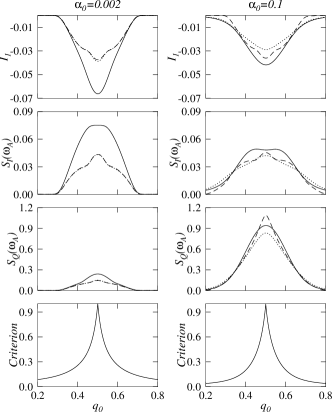
Figure 5: We plot the first harmonics of a tunneling current (in units of $E_{C}/eR_{T}$), current and charge noises (in units of $E_{C}/R_{T}$ and $e^{4}R_{T}/E_{C}$, respectively), and the criterion function as a function of gate charge $q_{0}$ for two sets of parameters. In the left column, tunneling resistances are chosen to be $R_{D}=R_{S}=655k\Omega$ ($\alpha_{0}=0.002$) and a frequency of a microwave $\hbar\omega_{A}\!=\!\hbar\omega_{R}=0.01$ while in the right column $R_{D}=R_{S}=13.1k\Omega$ ($\alpha_{0}=0.1$) and $\hbar\omega_{A}=0.2$ are used. We compare results calculated based on the exact, adiabatic, and orthodox formula by displaying them in solid, dotted and dashed lines, respectively. Other parameters are $k_{B}T=0.01$, $C_{D}=C_{S}=0.1$, $Q_{F}=6$, and $2Q_{F}ev_{in}=0.5$.

Fig. 5 shows calculated results of the currents and noises for the above two cases as a function of gate charge; for the smaller (large) in the left (right) column. In each column we additionally distinguish results depending on the formalism used; the exact (solid), adiabatic (dotted), orthodox (dashed) formalism, respectively. Thus, the differences between the exact and adiabatic results represent the existence of photon-assisted tunneling while those between adiabatic and orthodox results just emphasize effects of co-tunneling in the classical limit (for the small resistance the orthodox theory is known to be invalid, nevertheless we also show corresponding results just for comparison).

Figure 6: We plot the transmission function $T^{F}_{D}(t,t;E)$ at the drain with parameters used in Fig. (5)-(b). For gate charges of $q_{0}=0.2e$ and $0.5e$, its contour plot is depicted in $(a)$ and $(b)$, respectively. Here, a time $t$ is measured in units of a period of a microwave $T_{A}$.

From the calculated results, one can see that the system is easily driven into the non-adiabatic regime around the degeneracy point $q_{0}=e/2$ in both cases of tunneling resistances implying the fact that tunneling occurs in photon-assisted ways and, there, tunneling currents as well as noises are largely enhanced relative to the adiabatic results. This tendency is more apparent in the case of the large resistance. However, apart far from the degeneracy point, effects of time-dependent perturbations are reduced to classical ones to give nearly identical results independently of the formalism used. In other words, the strength of the photon-assisted tunneling becomes weak far from the degeneracy point.

One of possible explanations for the different strength of the photon-assisted tunneling depending on gate charges $q_{0}$ and tunneling resistances is the resolution of photon energies $\hbar\omega_{A}$ seen by particles. As inferred from Eq. (133) since particles in the island is decayed with a rate of $\gamma_{0}=\Im\Sigma^{A}(\Delta_{0})$, its dwelling time can be regarded to be inversely proportional to the rate. Along this aspect, the left-hand term in Eq. (134) can be interpreted as rough estimator of the resolution for energy quanta $\hbar\omega_{A}$. We plot it in the bottom panel of Fig. 5 for both cases of the tunneling resistances. According to the figure, when the value is less than about $0.1$, the calculations show nearly identical behavior between the adiabatic and exact results implying poor resolution for energy quanta. This fact is also confirmed by studying the transmission function $T^{F}$ of Eq. (123). Fig. 6 is a contour plot of the transmission function in the energy-time space for two different points of gate charges at which the resolution is predicted to be poor (at $q_{0}=0.2e$) and good (at $q_{0}=0.5e$) in Fig. 5-$(b)$. As shown in the figure, their time and energy dependences are strikingly complex. However, one can recognize the distinct feature different from each other. In $(a)$ for a given time the height of the transmission function is changed continuously as a function of energy while in $(b)$ it exhibits rather discrete behavior. Actually in the case of $(b)$ the distance between successive maximums is equal to photon energy of $\hbar\omega_{A}$, which is well resolved enough to see photon-side bands.

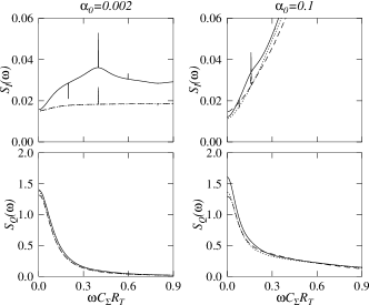
Figure 7: Under the same condition as those of Fig. 5, we plot the frequency dependence of current (top) and charge (bottom) noises for $\alpha_{0}=0.002$ (left) and $0.1$ (right panel), respectively. In each figure, results by the exact, adiabatic, and orthodox formula are represented by solid, dotted, and dashed lines, respectively, at a gate charge $q_{0}=0.4$ (current and charge noises are measured in units of $E_{C}/R_{T}$ and $e^{4}R_{T}/E_{C}$, respectively). Sharp peaks correspond to an infinite averaging time $T$ in Eq. (115), otherwise smeared ones may be obtained.

For the frequency dependences of the current and charge noises, we examine them at a gate charge $q_{0}=0.4e$ of Fig. 5 and show results in Fig. 7 in the range of low frequencies. In the current noises, the differences at a frequency $\omega=\omega_{A}$ between the adiabatic and exact results are found to be retained in the whole range of frequencies accompanying some structured behavior in both tunneling resistances. A straightforward explanation for these differences is complicated by various correlations among transport coefficients of $n_{\ell}$, $T^{F}_{\ell}$, $T^{R}_{\ell}$, and $L_{\ell}$ in Eq. (126) where they all are found to play roles somewhat importantly. As for peaks located at multiple of a frequency $\omega_{A}/2$, they are apparently arisen from time-dependent properties of external perturbations as noted in Eq. (152). Usually, the largest peak is found at $\omega=\omega_{A}$, however, in the exact results peaks at $\omega=\omega_{A}/2$ and $3\omega_{A}/2$ are also appreciable contrary to the adiabatic cases. This means that in photon-assisted ways the correlations between different harmonics of the above coefficients remain large while they are unimportant in the adiabatic limit. In the bottom of the figure, we show the charge noises as a function of frequency. Due to a large frequency scale we do not distinguish their differences clearly. However, in term of $\omega^{2}S_{Q}(\omega)$, we find that each result shows an appreciable deviation from the others. Actually, the function of $\omega^{2}S_{Q}(\omega)$ is related to the current noises because the last term of Eq. (126) is approximately equal to it neglecting geometrical factors between capacitances. By comparing it with the current noises, we find that a large portion of the difference in the current noise can be associated with those in the charge noises.

For high frequencies, the noises are found to be nearly identical to equilibrium noises calculated with no external perturbations. Namely, the Johnson-Nyquist noises are dominant.

V.3 Charge sensitivity

The sensitivity to gate charges is one of estimators for the performance of a rf SET as an electrometer. If one measures the amplitude $X$ assuming a homodyne detector, the charge sensitivity is calculated as,averin ; turin

$$\delta q=\frac{\sqrt{S_{XX}(\omega_{A})}}{\mid dX/dq_{0}\mid}=\frac{\sqrt{2S_{I}(\omega_{A})}}{\mid dI_{1}/dq_{0}\mid},$$ (154)

showing the dependence on the current noises $S_{I}$ and the response function $dI_{1}/dq_{0}$.

Figure 8: Contour plots of the charge sensitivity $\delta q$ (in units of $e\sqrt{\hbar/E_{C}}$) in the space of rf amplitudes and gate charges are shown. The used parameters are $\hbar\omega=0.04E_{C}$, $Q_{F}=6$, and $R_{D}=R_{S}=100k\Omega$ at a temperature of $k_{B}T=0.02E_{C}$.

In Fig. 8 we plot the sensitivity in the $q_{0}$-$v_{in}$ plane using the three different formula. Aiming at the simulation of Ref. schoel , we use similar system parameters to the experiment except for $C_{D}=C_{S}=0.1$ (unfortunately not specified in the experiment). To clarify calculated results we omit the regions of poor sensitivity, which correspond to smaller rf-wave amplitudes than the Coulomb blockade thresholds (lower left corner) and much higher rf-wave amplitude over the threshold with small excitation energies (upper right corner). By comparing Fig. 8-(a) and (b), one can see effects of photon-assistant tunneling to the sensitivity. That is, the region of good sensitivity (for example, within $\delta q=2.5$) is predicted to slowly vary as a function of rf-wave amplitude than in the adiabatic limits, while it exhibits a rather narrower region as a function of gate charge. Calculated optimum sensitivities (minimum value of $\delta q$) are also found to have different values, $\delta q=2.12,2.38$, and $1.83$ for the exact, adiabatic, and orthodox formalism, respectively, with a nearly same operating point of $(q_{0},2Q_{F}v_{in})=(0.47,0.12\sim 0.17)$. The slightly better optimum-sensitivity in Fig. 8-$(a)$ compared with that in $(b)$ comes from the enhanced value of the response $dI_{q}/dq_{0}$ by photon-assisted tunneling. However, photon-assisted tunneling does not always give the better sensitivity because it also enhances current noises. We find that its role for the sensitivity depends on system parameters. In the orthodox result, the sensitivity is always predicted to be better than results of the others because the absence of co-tunneling gives larger values of the response $dI_{q}/dq_{0}$.

Using the experimental parameter of $E_{C}=178\mu eV$, the calculated optimum sensitivity $\delta q=2.12$ corresponds to $4.1\mu e/\sqrt{{\rm Hz}}$, which is lower than the measured value of $47\mu e/\sqrt{{\rm Hz}}$ by an order. This discrepancy between the theory and experiment may be attributed to the preamplifier noise and local heating of a SET.turin

Figure 9: The optimum charge sensitivities are plotted as a function of tunneling resistance for two quality factors of $Q_{F}=6$ in $(a)$ and $50$ in $(b)$, respectively, together with different frequencies of a microwave, $\hbar\omega_{A}=0.1$ (dotted), $0.04$ (solid), and $0.005$ (dashed). The dot-dashed lines denote the analytical result of Eq. (155). Here, we assume $R_{S}=R_{D}$, $C_{D}=C_{S}=0.1$, and $k_{B}T=0.02$. In (c) we re-plot the result of (b) represented by the solid line, and examine its change without each calculational factor one by one; adiabatic approximation (dotted line), no electrical environment (square), symmetric geometry of $C_{D}=C_{S}=0.24$ (dashed line), and calculation neglecting a self-consistency (triangle).

In Fig. 9, we show the dependence of the optimum sensitivity on tunneling resistances for different applied frequencies of microwaves and quality factors. Firstly, Figs. 9-$(a)$ and $(b)$ are results for $Q_{F}=6$ and $50$, respectively. By comparing different kinds of lines in each figure which means different frequencies of microwaves at a resonant condition, one can see that larger frequencies give rise to worse sensitives in a wide range of tunneling resistance. Since a large driving frequency corresponds to better-resolved energies of external fields, associated photon-assisted tunneling is expected to decrease the sensitivity due to the enhanced current noises. On the other hand, for a given frequency, the sensitivity as a function of tunneling resistance is found to show different behavior depending on the quality factor; monotonically improved results are obtained for $Q_{F}=6$ as tunneling resistance decreases while there is optimal resistance for the best sensitivity for $Q_{F}=50$. For easier understanding of our results, an analytic expression from Ref. turin ,

$$\delta q\sim 2.65e\sqrt{(R_{D}\!+\!R_{S})C_{\Sigma}}\sqrt{\frac{k_{B}T}{2E_{C}}}$$ (155)

is also plotted with dot-dashed lines in the figure even though it gives difference values from ours due to the orthodox theory. According to this expression, since the sensitivity is proportional to $\alpha_{0}^{-1/2}$ for $R_{D}=R_{S}$, one can see that calculated results are approximately scaled as the same power law. However, for $Q_{F}=50$, the power law is no longer hold and for small tunneling resistances it is scaled as even $\alpha_{0}^{1/2}$. This behavior can be understood through a simple circuital analysis as in Ref. turin By replacing the tunneling barriers by resistors, it is found that the best sensitivity is achieved for series resistance equal to $Q_{F}^{2}R_{0}$ at which input impedance of microwaves is matched to that of the tunneling barriers. Thus, for $Q_{F}=6$ the matching condition occurs at $\alpha_{0}=1.5$ while for $Q_{F}=50$ it is expected to be $\alpha_{0}=0.02$. As shown in Fig. 9-$(b)$, this condition well agrees with the calculated result for the small frequency even though for high frequencies it is slightly deviated due to the non-adiabatic effects of microwaves.

In Fig. 9-$(c)$ we show the dependence of the charge sensitivity on tunneling resistances by omitting a calculational factor one by one to emphasize its role. According to results, considerations of self-consistent and non-adiabatic schemes are found to be crucial for sensitivity calculations while effects of the environment is relatively unimportant. In addition, we find that symmetric geometry (dashed line) benefits the charge sensitivity in the whole range of tunneling resistance.

VI Summary

In this work, we develop a formalism for a radio-frequency single-electron transistor taking into account electrical environment, higher-order co-tunneling, and arbitrary time-dependent perturbations. Assuming large charging energy, we use a two-charged-state model in a metallic island and solved the problem based on the Schwinger-Keldysh approach combined with a generating functional method. We calculate an approximated generating functional by summing diagrams in infinite order and give exact expressions for current, charges in the island, and their noises within the generating functional. By defining generalized transport coefficients, we write the derived expressions in terms of them, and show that tunneling currents in time-dependence cases have a generalized form of the well-known Landauer formula.

As application of our formalism, we examine tunneling currents, its noises, and the charge sensitivity of rf-SETs by accounting for a detailed tank circuit. Firstly, effects of the electrical environments are found to be relatively small, as expected, in cases of microwaves delivered via an coaxial cable with impedance $50\Omega$. However, for a large quality factor and a large resonant frequency its effects become large and cannot be ignored. Secondly, effects of photon-assisted tunneling are manifested to both enhanced responses and noises of rf SETs. However, due to the larger enhancement of the noises, photon-assisted tunneling is not helpful to the charge sensitivity. As a consequence, with experimental parameters of Ref. schoel , we obtain the charge sensitivity of $\delta q=4.1\mu e/\sqrt{{\rm Hz}}$, which is larger than that in the orthodox result, however, still much smaller than the measure value of $47\mu e/\sqrt{\rm Hz}$. Finally, we discuss the charge sensitivity depending on various sets of parameters. Especially, we focus on its change as a function of tunneling resistance, and find that the charge sensitivity for small quality factors is scaled like $\alpha_{0}^{-1/2}$ as in the analytic result proposed by the previous work. Whereas, for large quality factors the power law is no longer valid and it is proportional to even $\alpha_{0}^{1/2}$ in the range of small tunneling resistance to show optimal resistance for the best sensitivity.

- (1) H. van Houten, C. W. J. Beenakker, and A. A. M. Staring, NATO ASI Ser., B 294, 167 (1991).
- (2) D. V. Averin, K. K. Likharev, in Mesoscopic Phenomena in Solids, edited by B. L. Altshuler, P. A. Lee, and R. A. Webb (Elsevier Science Publishers B. V., Amsterdam, 1991).
- (3) G. Ingold and Y. V. Nazarov, Single Charge Tunneling, edited by H. Grabert and M. H. Devoret, Plenum Press, New York, (1992).
- (4) L. P. Kouwenhven and P. L. McEuen, in Nano-Science and Technology, edited by G. Timp (AIP press 1997).
- (5) G. Schön, in Quantum transport and Dissipation, edited by T. Dittrich, P. Häggi, G. Ingold, B. Kramer, G. Schön, and W. Zwerger (Wiley-VCH, Weinheim, 1998).
- (6) C. W. J. Beenakker, Phys. Rev. B 44, 1646 (1991).
- (7) H. Schoeller and G. Schön, Phys. Rev. B 50, 18436 (1994).
- (8) D. V. Averin, in Macroscopic Quantum Coherence and Quantum Computing, edited by D. V. Averin, R. Ruggiero, and P. Silvestrini (Kluwer Academic/Plenum Publisher, New York, 2001).
- (9) E. V. Sukhorukov, G. Burkard, and D. Loss, Phys. Rev. B 63, 125315 (2001).
- (10) Y. Utsumi, H. Imamura, M. Hayashi, and H. Ebisawa, Phys. Rev. B 66, 024513 (2002); ibid, Phys. Rev. B 67, 035317 (2003).
- (11) Y. Makhlin, G. Schön, and A. Shnirman, Phys. Rev. Lett. 85, 4578 (2000).
- (12) B. E. Kane, N. S. McAlpine, A. S. Dzurak, R. G. Clark, G. J. Milburn, H. B. Sun, and H. Wiseman, Phys. Rev. B 61, 2961 (2000).
- (13) A. Aassime, G. Johansson, G. Wendin, R. J. Schoelkopf, and P. Delsing, Phys. Rev. Lett. 86, 3376 (2001).
- (14) G. Johansson, A. Käck, and G. Wendin, Phys. Rev. Lett. 88, 046802 (2002).
- (15) R. J. Schoelkopf, P. Wahlgren, A. A. Kozhevnikov, P. Delsing, D. E. Prober, E. Abrahams et al., Science, 280, 1238 (1998).
- (16) T. Fujisawa and Y. Hirayama, Appl. Phys. Lett. 77, 543 (2000).
- (17) H. D. Cheong, T. Fujisawa, T. Hayashi, Y. Hirayama, and Y. H. Jeong, Appl. Phys. Lett. 81, 3257 (2002).
- (18) T. M. Buehler, D. J. Reilly, R. P. Starret, A. R. Hamilton, A. S. Dzurak, and R. G. Clark, cond-mat/0302085.
- (19) P. K. Tien and J. R. Gordon, Phys. Rev. 129, 647 (1963).
- (20) L. P. Kouwenhoven, S. Jauhar, J. Orenstein, P. L. McEuen, Y. Nagamune, J. Motohisa, and H. Sakaki, Phys. Rev. Lett. 73, 3443 (1994).
- (21) C. Bruder and H. Schoeller, Phys. Rev. Lett. 72, 1076 (1994).
- (22) C. A. Stafford and N. S. Wingreen, Phys. Rev. Lett. 76, 1916 (1996).
- (23) J. H. Oh, D. Ahn, and S. W. Hwang, Phys. Rev. B 68, 205403 (2003);
- (24) M. H. Devoret, D. Esteve, H. Grabert, G. Ingold, H. Pothier, and C. Urbina, Phys. Rev. Lett. 64, 1824 (1990).
- (25) H. Grabert, G. Ingold, M. H. Devoret, D. Esteve, H. Pothier, and C. Urbina, Z. Phys. B-Condensed Matter, 84, 143 (1991).
- (26) J. H. Oh, H. Lee, S. W. Hwang, and D. Ahn, J. Korean Phys. Soc. 45, S589 (2004).
- (27) A. Jauho, N. S. Wingreen, Y. Meir, Phys. Rev. B 50, 5528 (1994);
- (28) S. Camalet, J. Lehmann, S. Kohler, and P. Hánggi, Phys. Rev. Lett. 90, 210602 (2003).
- (29) J. W. Negele and H. Orland, Quantum Many-particle Systems, (Addison-Wesley publishing company, 1988).
- (30) K. Chou, Z. Su, B. Hao, and L. Yu, Phys. Rep. 118, 1 (1985).
- (31) V. S. Babichenko and A. N. Kozlov, Solid State Commun. 59, 39 (1986).
- (32) A. O. Caldeira and A. J. Leggett, Ann. Phys. (N.Y.), 149, 374 (1983).
- (33) R. Landauer, IBM J. Res. Dev., 32, 306 (1988).
- (34) A. J. Rimberg, T. R. Ho, C. Kurdak, J. Clarke, K. L. Campman, and A. C. Gossard, Phys. Rev. Lett. 78, 2632 (1997).
- (35) N. Mason and A. Kapitulnik, Phys. Rev. Lett. 82, 5341 (1999).
- (36) J. S. Penttilä, Ü. Parts, P. J. Hakonen, M. A. Paalanen, and E. B. Sonin, Phys. Rev. Lett. 82, 1004 (1999).
- (37) A. Shnirman and G. Schön, Phys. Rev. B 57, 15400 (1998).
- (38) J. H. Davies, P. Hyldgaard, S. Hershfield, and J. W. Wilkins, Phys. Rev. B 46, 9620 (1992).
- (39) U. Hanke, Y. M. Galperin, K. A. Chao, and N. Zou, Phys. Rev. B 48, 17209 (1993).
- (40) A. N. Korotkov, Phys. Rev. B 49, 10381 (1994).
- (41) M. Büttiker, J. of Low Temp. Phys. 118, 519 (2000).
- (42) V. O. Turin and A. N. Korotkov, Phys. Rev. B 69, 195310 (2003); ibid, Appl. Phys. Lett. 83, 2893 (2003).
- (43) L. Roschier, P. Hakonen, K. Bladh, P. Delsing, K. W. Lehnert, L. Spietz, and R. Schoelkopf, J. Appl. Phys. 95, 1274 (2004).