Granular Packings: Nonlinear elasticity, sound propagation and collective relaxation dynamics

Abstract

Experiments on isotropic compression of a granular assembly of spheres show that the shear and bulk moduli vary with the confining pressure faster than the $1/3$ power law predicted by Hertz-Mindlin effective medium theories (EMT) of contact elasticity. Moreover, the ratio between the moduli is found to be larger than the prediction of the elastic theory by a constant value. The understanding of these discrepancies has been a longstanding question in the field of granular matter. Here we perform a test of the applicability of elasticity theory to granular materials. We perform sound propagation experiments, numerical simulations and theoretical studies to understand the elastic response of a deforming granular assembly of soft spheres under isotropic loading. Our results for the behavior of the elastic moduli of the system agree very well with experiments. We show that the elasticity partially describes the experimental and numerical results for a system under compressional loads. However, it drastically fails for systems under shear perturbations, particularly for packings without tangential forces and friction. Our work indicates that a correct treatment should include not only the purely elastic response but also collective relaxation mechanisms related to structural disorder and nonaffine motion of grains.

I Introduction and Objectives

The acoustic properties of granular porous materials confined by an external stress can be extremely nonlinear as compared to continuum elastic solids powders ; goddard ; guyer ; hans0 . Many industrial applications, such as the optimization of well location in an oil reservoir, depend crucially on the correct interpretation of nonlinear acoustic effects in granular materials, as exemplified by the large variation of the sound speeds or the elastic constants of the granular formation as a function of the external stress sinha ; footnote .

Important insight into this problem comes first from the Hertz-Mindlin contact theory to model the intergrain forces johnson ; landau . In this case, nonlinearity arises from the increase with the external stress of the contact area between two spherical grains. Conventional theories describing this problem in the framework of elasticity of continuum media landau consider a uniform strain at all scales, and the displacement field of the grains is affine with the macroscopic deformation (the affine approximation). Here, one computes the stresses in terms of the strains by considering the disordered medium as an effective medium that exerts a mean-field force (as given by contact Hertzian theory) on a single representative grain. This approximation is usually referred to as the Effective Medium Theory (EMT) mindlin2 ; digby ; walton ; johnson1 .

As shown in a short letter mgjs and the studies of other groups goddard , the EMT does not successfully explain the mechanical properties of cohesionless granular assemblies. The main prediction of the theory is the scaling of the bulk modulus, $K$, and shear modulus, $\mu$, with the pressure, $p$, as $K\sim\mu\sim p^{1/3}$. However there is a large volume of experiments for irregular sand grains as well as spherical glass beads which show anomalous scaling characterized by exponents varying between $1/3$ and $1/2$ (for a comprehensive review see Goddard goddard and for a review in the geotechnical literature see woods ). Some studies have suggested that a $\sim p^{1/2}$ scaling is more appropriate for describing the nonlinear variation of the moduli goddard .

Here we extend the results of mgjs and investigate the applicability of elasticity theory to granular matter by means of experiments, computer simulations, and analytical calculations. We first develop a series of acoustic experiments to characterize the nonlinear elastic behavior of non-cohesive dry granular materials under a wide range of external pressures. From this experimental study we conclude that a microscopic study is needed in order to elucidate the deficiencies of existing granular theories. Then we perform a Molecular Dynamics (MD) simulation to give microscopic insight into the relaxation mechanism of granular materials. Finally, we offer a simple theory of relaxation going beyond the effective medium approximation of elasticity.

We calculate the elastic moduli, $K$ and $\mu$, of a disordered array of elasto-frictional Hertz-Mindlin spherical grains. Numerical simulations resolve the question as to whether the problem lies in the treatment of intergrain contact or with the EMT. We find agreement between our simulations and the experiments, thus confirming the validity of the Hertz-Mindlin contact theory to glass bead aggregates composed of frictional particles.

Regarding the anomalous pressure dependence of the moduli, we find that there are several nonlinearities which preclude the proper definition of a scaling behavior as a function of pressure. We find a regime at low pressure where the coordination number and the volume fraction do not change much from their minimal values. In this regime the $p^{1/3}$ scaling is approximately valid. However, for pressures larger than 10 MPa the increase of the coordination number and volume fraction induces other nonlinearities and therefore no simple scaling behavior can be defined.

In reality around 10 MPa there is crossover from a $p^{1/3}$ to a $p^{5/9}$ scaling at larger pressures. Thus, we conclude that the scattering in the experimental values of the pressure exponent might be explained by the fact that the exponent is actually changing continuously from 1/3 to 5/9. This is especially true in the regime where the experiments are usually done, near the crossover region at 10 MPa. Similar conclusions have been reached by Luding luding who also found that EMT needs to take into account the coordination number and its dependence on pressure.

Our most important results relate to the effect of friction and stress relaxation on the behavior of the elastic constants. Firstly, we find that the elastic formulation gives a reasonable description for the response of the system to compressional loads, i.e. the bulk modulus is reasonably well defined with the simple EMT. However, our simulations establish that the EMT is inadequate in describing the response of the material under shear perturbations.

The numerical simulations indicate that EMT fails because it does not properly allow the grains to relax from the affine deformation imposed by the external boundary. The affine assumption is that, under an infinitesimal symmetric macroscopic deformation, each grain translates according to the direction of the macroscopic strain, and it does not rotate. Moreover, no further relaxation mechanism is allowed. Such an homogeneous strain field is consistent with the local force balance of grains only in an ordered system. For disordered packings an inhomogeneous strain develops at the local level. After the application of an affine strain the particles experience an unbalanced force since they are not, in general, in a symmetric environment. Consequently, the particles will move to a position different to that predicted by the affine approximation, so that the net force on each particle is zero. Similarly for torques and rotations.

Here we show that the assumption of affinity is approximately valid for the bulk modulus and seriously flawed for the shear modulus. For this reason, the EMT prediction differs significantly from the experimental value. Thus, the principal source of deviation from EMT is the breakdown of the uniform strain assumption.

To quantify the breakdown of EMT for the shear modulus we focus our studies to two cases: frictionless grains interacting via only normal forces (this system is said to be path-independent and it is thought to describe compressible foams and emulsions) and systems with elastic tangential forces and Coulomb frictional forces (these systems are path-dependent and describe dry granular materials).

The largest disagreement between theory and simulations is found for frictionless systems; the difference is more pronounced at low confining stress where we show that the system is in a state of marginal rigidity at a minimal mean coordination number equal to 6 in 3D (or 4 in 2D). We find that after the application of an external shear strain there is a nearly complete relaxation of the system to the applied shear; a result that cannot be captured under the framework of elasticity. We show that a new scaling behavior with pressure might describe the data for frictionless particles better: $\mu(p)\sim p^{2/3}$ as $p\to 0$.

We interpret this result in the framework of critical phenomena: as $p\to 0$ the system approaches a critical point at a mean coordination number $Z_{c}=2D$ in $D$ dimensions, and a volume fraction of random close packing $\phi_{c}\approx 0.64$. This point describes a rigidity threshold state or a critical state of the packing as defined by Alexander alexander and it is where the system becomes “isostatic” isostatic ; edwards-grinev ; ball . The elastic moduli vanish as a power-law of the pressure or volume fraction. For any finite pressure rigidity is achieved, since $Z>Z_{c}$. Near the rigidity threshold the reference packing structure has a power law dependence on the pressure, modifying the scaling of $\mu(p)$ predicted by the Hertz theory.

When friction and tangential elasticity is restored at the intergrain contacts, the agreement between theory and simulations (and in this case experiments) improves with respect to the frictionless case. This is because the existence of tangential restoring forces reduces the extent to which the grains relax from the assumed affine configuration. Thus, the EMT provides a better agreement with simulations and with experiments for frictional grains than for frictionless grains, but serious disagreements still persist as we shall demonstrate.

We conclude that in order to develop a better understanding of the problem, one must abandon the purely elastic framework and consider granular matter as a full viscoelastic body. Collective relaxation effects can account for the discrepancy in the shear modulus in comparison with the elastic prediction: the corrections increase dramatically in the case of loose materials and for frictionless packings. A theory of single-particle relaxation is offered as a first step in this direction. We also discuss our results in the framework of recent theories of marginal rigidity, jamming, melting and fragile matter.

Applications.– Part of the motivation for this research derives from the fact that acoustics and nonlinear elastic logging methods are at the forefront of the evolving technology to help plan and optimize well location in oil exploration oilfield . In order to position a well correctly, the knowledge of the stress distribution around the borehole is essential. Mechanical properties of the granular formation obtained from sonic logging can help predict formation strength, while stress magnitude derived from sonic measurements helps in predicting sanding problems in unconsolidated formations. Acoustic measurements in granular materials provide the natural way to understand the distribution of stress around the borehole.

Quite apart from the relevance to borehole logging, within the field of seismic tomography there is a growing interest in developing techniques to generate images of dissipation, along with the more traditional images of impedance contrast. This extended seismic tomography would have impact, not only on the understanding of hydrocarbon reservoirs but also e.g. on techniques to monitor the migration of ground water pollutants. This work represents an attempt to understand some of the mechanisms of attenuation as well as the stress dependence of sound velocities in granular materials.

The outline of the paper is as follows. Section II reviews the background of the problem of Effective Medium theories and numerical approaches: MD simulations and intergrain forces for granular materials, compressed emulsions and foams. Section III describes the experiments on sound propagation. Section IV describes the numerical results and Section V the theoretical results. We conclude in Section VI with a final outlook.

II Background

The problem of elastic properties of granular materials has been treated by many researchers since the pioneering work of Mindlin in the 50’s goddard ; mindlin2 ; domenico ; yin ; winkler ; ishibashi ; liu1 ; jussieu ; pgg ; jenkins ; nesterenko ; hascoet . However, a general solution to this problem is still lacking.

In a typical experiment, a set of cohesionless glass beads is confined at a hydrostatic stress, $p$, and the compressional sound speed, $v_{p}$, and the shear sound speed, $v_{s}$, are measured as functions of stress (see for instance Domenico domenico , Yin yin , and goddard ; winkler ; jussieu ). The P-wave and S-wave speeds are related to the elastic constants of the material in the long-wavelength limit:

$$v_{p}=\sqrt{\frac{K+4/3\mu}{\rho}},$$ (1)

$$v_{s}=\sqrt{\frac{\mu}{\rho}},$$ (2)

where $\rho$ is the mass density of the system.

II.1 Contact mechanics.

In his seminal paper “On the Contact of Elastic Solids” H. Hertz johnson ; landau used linear elasticity of continuum media to calculate the normal force of two perfectly elastic spheres pressed into contact considering no attraction or stickiness. Hertz showed that two spherical grains in contact with radii $R_{1}$ and $R_{2}$ interact with a normal repulsive force

$$F_{n}=\frac{2}{3}~{}k_{n}R^{1/2}\xi^{3/2},$$ (3)

where $R=2R_{1}R_{2}/(R_{1}+R_{2})$, the normal overlap is $\xi=(1/2)[(R_{1}+R_{2})-|\vec{x}_{1}-\vec{x}_{2}|]>0$, and $\vec{x}_{1}$, $\vec{x}_{2}$ are the positions of the grain centers. The normal force acts only in compression, $F_{n}=0$ when $\xi<0$. The effective stiffness $k_{n}=4\mu_{g}/(1-\nu_{g})$ is defined in terms of the shear modulus of the grains $\mu_{g}$ and the Poisson ratio $\nu_{g}$ of the material from which the grains are made (typically $\mu_{g}=29$ GPa and $\nu_{g}=0.2$, for spherical glass beads).

The situation in the presence of a tangential force, $F_{t}$, is more complicated. In the case of spheres under oblique loading, the tangential contact force was first calculated by Mindlin mindlin . A general loading history can be described by the incremental change in the tangential force $\Delta F_{t}$ and in the normal force $\Delta F_{n}$. For the special case where the partial increments do not involve microslip at the contact surface (i.e., $|\Delta F_{t}|<\mu_{f}\Delta F_{n}$, where $\mu_{f}$ is the kinematic friction coefficient between the spheres, typically $\mu_{f}=0.3$) Mindlin mindlin showed that the tangential force is

$$\Delta F_{t}=k_{t}(R\xi)^{1/2}\Delta s,$$ (4)

where $k_{t}=8\mu_{g}/(2-\nu_{g})$, and the variable $s$ is defined such that the relative shear displacement between the two grain centers is $2s$. This is called the Mindlin “no-slip” solution. [See Appendix A for a more general solution].

The incremental form Eq. (4) is needed since the numerical value of the tangential force depends upon the trajectory taken in the space ($\xi,s$), see johnson1 for details. The tangential force is obtained by integrating over the path taken by the spheres in contact subject to the initial conditions: $F_{n}=0$, $F_{t}=0$ at $\xi=0,s=0$, yielding:

$$F_{t}=\int_{path}k_{t}(R\xi)^{1/2}ds.$$ (5)

Thus, a granular system with tangential elastic forces is said to be path-dependent. By path dependency we mean that the work done in deforming the system depends upon whether one first compresses the system, then shears it, or first shears it then compresses. The results depend upon the path taken and not just the instantaneous final state. On the other hand, a system of spheres interacting only via normal forces, Eq. (3), is said to be path-independent, and the work does not depend on the way the strain is applied.

As the shear displacement increases, the elastic tangential force $F_{t}$ reaches its limiting value given by Amontons’ law for no adhesion, $F_{t}\leq\mu_{f}F_{n}$. Amontons’ law (a special case of Coulomb’s law) adds a second source of path-dependency as well as hysteresis to the problem.

II.2 Effective medium theories (EMT) of granular elasticity

The basic idea of elastic theories relevant to our study is that the macroscopic work done in deforming the system is set equal to the sum of the work done on each grain-grain contact and that the latter is replaced by a suitable average digby ; walton ; johnson1 . These theories are usually referred to as the effective medium theory (EMT) and are based on Hertz-Mindlin contact mechanics. In the case of an isotropic deformable solid (for simplicity we describe the isotropic case), the strain energy density per unit volume as a function of the strain $\epsilon_{ij}$ is:

$$U(\epsilon_{ij})=U_{0}-p\epsilon_{ll}+\mu_{e}(\epsilon_{ij}-\frac{1}{3}\delta_{ij}\epsilon_{ll})^{2}+\frac{1}{2}K_{e}(\epsilon_{ll})^{2}+O(\epsilon_{ij}^{3})\>\>\>.$$ (6)

This equation is equivalent to the expression

$$\sigma_{ij}=K_{e}\epsilon_{ll}\delta_{ij}+2\mu_{e}(\epsilon_{ij}-\frac{1}{3}\delta_{ij}\epsilon_{ll}),$$ (7)

which determines the stress tensor $\sigma_{ij}$ in terms of the strain tensor for an isotropic body landau . Here

$$\epsilon_{ij}=1/2(\partial u_{i}/\partial x_{j}+\partial u_{j}/\partial x_{i}),$$ (8)

and the deviations $u_{i}=x_{i}-R_{i}$ of the positions of the $N$ particles in the system, {x${}_{1},\ldots,$ x_N} , are measured from a suitable rigid reference state

$$\mbox{ \bf{\{R\} = \{R${}_{1}$,\ldots, R${}_{N}$\} } },$$ (9)

around which one can expand consistently. This reference state is straightforward for simple periodic systems. However, it is assumed that this expansion is also possible for amorphous solids with reference states which are random, like in a packing of grains (see Alexander alexander for extensive discussions). The subscript in $K_{e}$ and $\mu_{e}$ denotes that the values of the moduli are calculated considering granular materials as purely elastic solids. There are two assumptions inherent to the elastic EMT:

• All the spheres are statistically the same, and it is assumed that there is an isotropic distribution of contacts around a given sphere.

• An affine approximation is used, i.e., the spheres at position $x_{j}$ are moved a distance $\delta u_{i}$ in a time interval $\delta t$ according to the macroscopic strain rate $\dot{\epsilon}_{ij}$ by

  $$\delta u_{i}=\dot{\epsilon}_{ij}x_{j}\delta t.$$ (10)

  The grains are always at equilibrium due to the assumption of an isotropic distribution of contacts, and further relaxation is not required. This sort of mean field theory is analogous to a simple average of non-linear spring constants.

It is important to notice that a definition of uniform strain field is possible only under the mean field approximation. This assumption is also trivially correct for ordered packings. However, for disordered systems, the affine approximation is inconsistent with the local equilibrium of grains green3 . We will come back to this crucial point later on.

With the above assumptions, the elastic energy Eq. (6) is set equal to a suitable average over the contacts, viz:

$$U=\frac{1}{V}\sum_{contact}\int\mbox{\bf F $\cdot$ $d$u}\approx\frac{Z\phi}{V_{0}}\langle\int\mbox{\bf F $\cdot$ $d$u}\rangle,$$ (11)

with $\mbox{\bf F}\cdot d\mbox{\bf u}=F_{n}d\xi+\mbox{\bf F}_{t}\cdot d\mbox{\bf s}$, $Z$ is the average coordination number defined as the average number of contacts per particle, $\phi$ is the volume fraction of the sample, and $V_{0}$ is the volume of a single grain. The EMT predictions for the bulk and shear modulus for an isotropic system compressed at pressure $p$ are the following:

We distinguish between two different models:

(1)Path-independent models, $k_{t}=0$, frictionless grains: We consider that there is perfect slippage at the intergrain contact. This corresponds to $F_{t}=0$, only normal forces between the particles. This case corresponds to path-independent forces, and allows the use of an energy density function Eq. (6) which depends only on the instantaneous position of the particles. This case could be considered conservative since the total work on a closed path is zero. A system of frictionless spherical particles could be thought of as a model of compressed emulsions and foams which are usually modeled as viscoelastic spheres without tangential forces lacasse ; durian ; faraday (see Appendix C).

For the case of frictionless grains one finds:

$$K_{e}(p)=\frac{k_{n}}{12\pi}~{}(\phi Z)^{2/3}~{}\left(\frac{6\pi p}{k_{n}}\right)^{1/3},$$ (12)

$$\mu_{e}(p)=\frac{k_{n}}{20\pi}~{}(\phi Z)^{2/3}~{}\left(\frac{6\pi p}{k_{n}}\right)^{1/3}.$$ (13)

(2) Path-dependent models, $k_{t}\neq 0$, frictional grains: In this case tangential elastic forces are taken into consideration. In principle the energy functional (6) now depends on the path. However, it has been shown that the second order elastic constants are still path-independent under the framework of EMT, while path-dependency appears only in the third order elastic constants johnson1 .

The bulk modulus is not affected by the introduction of tangential forces, and Eq. (12) is still valid in this case. However, the shear modulus is modified according to:

$$\mu_{e}(p)=\frac{k_{n}+\frac{3}{2}k_{t}}{20\pi}~{}(\phi Z)^{2/3}~{}\left(\frac{6\pi p}{k_{n}}\right)^{1/3}.$$ (14)

The above results have been obtained by a number of authors using different methods and are valid in 3-D digby ; walton ; johnson1 . It should be noted that the above results are obtained for a system of infinitely rough spheres, i.e. when $\mu_{f}\to\infty$. Thus, there is no sliding, and Coulomb friction is not considered, although there is a tangential elastic restoring force as given by Eq. (4). See Appendix A for further discussion.

The $p^{1/3}$ dependence in Eqs. (12)-(14) is a direct consequence of the scaling of the normal Hertz force on the deformation. Since

$$p\sim F_{n}\sim\xi^{3/2}\sim\epsilon^{3/2}.$$ (15)

Then we expect

$$\mu_{e}\sim K_{e}\sim\frac{\partial p}{\partial\epsilon}\sim\epsilon^{1/2}\sim p^{1/3}.$$ (16)

We note that a system of linear springs, $F_{n}\sim\xi$, would give rise to elastic constants which are independent of pressure, as in the linear elasticity theory.

II.3 Discrepancies between theory and experiments.

It was found experimentally that the shear and bulk moduli of an assembly of spherical grains vary with the confining stress, $p$, faster than the $p^{1/3}$ power law predicted by Eqs. (12)-(14) goddard . Another way of seeing the breakdown of the elastic theory is to focus on the ratio $K/\mu$. According to Eqs. (12) and (14) for frictional grains

$$\frac{K_{e}}{\mu_{e}}=\frac{5(2-\nu_{g})}{3(5-4\nu_{g})},$$ (17)

independent of stress, a value which depends only on the Poisson ratio of the bead material. The experiments give $K/\mu\approx 1.1-1.3$ domenico ; yin . EMT predicts $K_{e}/\mu_{e}=0.71$, if we take $\nu_{g}=0.2$ for the Poisson ratio of glass. [The EMT prediction is rather insensitive to variations of $\nu_{g}$; $K_{e}/\mu_{e}=0.71\pm 0.04$ for $\nu_{g}=0.2\pm 0.1$.] Conversely, a value $\nu_{g}\simeq 1.2$ would be needed in order to fit the experimental $K/\mu$, clearly violating the upper thermodynamic limit of $\nu_{g}\leq 1/2$ landau .

Another quantity of interest is the effective Poisson ratio of the pack $\nu$. According to EMT, $\nu_{e}$ is again independent of pressure and given only in terms of the Poisson’s ratio of the grains:

$$\nu_{e}\stackrel{{\scriptstyle def}}{{=}}\frac{K_{e}-2/3\mu_{e}}{2(K_{e}-1/3\mu_{e})}=\frac{\nu_{g}}{2(5-3\nu_{g})}.$$ (18)

Thus, for typical glass beads ($\nu_{g}=0.2$) we find a predicted value of $\nu_{e}=0.02$ which is one order of magnitude smaller than typical experimental values $\nu\approx 0.28$ domenico ; another serious disagreement.

The origin of the above discrepancies has not been clear: it could be due to the breakdown of the Hertz-Mindlin force law at each grain contact, or it could be associated with the breakdown of the elasticity theory applied to granular systems. De Gennes pgg proposed that a thin shell of oxide layer would give a faster growth with stress of the elastic moduli of the system, which may explain the behavior for metallic beads. Goddard goddard proposed that sharp angularities of the grains (for instance sand grains) may modify the contact force law between grains, giving rise to a different stress dependence. Other authors goddard ; jenkins have suggested that the increasing number of contacts with stress may be the reason for the discrepancies in the stress dependence of the moduli. Jenkins et al. jenkins measured the elastic moduli using numerical simulations for a single pressure and concluded that EMT does not correctly describe the shear modulus but it describes the bulk modulus fairly well. Other experimental work done by Liu and Nagel liu1 and Jia et al. jussieu concentrated on the role played by force chains in sound propagation. Different approaches for one dimensional elastic chains have also been applied to wave propagation in granular media nesterenko ; hascoet .

II.4 Linear viscoelastic constitutive models

In order to understand our results it is important to generalize the elastic concepts introduced above to the full viscoelastic response. In linear viscoelasticity ferry , the current state of stress specified by the stress tensor $\sigma_{ij}$ is determined by the past history via a linear constitutive equation

$$\sigma_{ij}(t)=\int_{-\infty}^{t}G_{ijkl}(t-t^{\prime})~{}\dot{\epsilon}_{kl}(t^{\prime})~{}dt^{\prime},$$ (19)

where $\dot{\epsilon}_{kl}=\partial\epsilon_{kl}/\partial t$ is the strain rate, and $G_{ijkl}(t)$ is called the relaxation modulus tensor.

For an isotropic linear viscoelastic material, the relaxation modulus tensor has only two independent components. These are the shear relaxation modulus $G(t)$ and the bulk relaxation modulus $K(t)$ characterizing the response to shear $\dot{\epsilon}_{12}$ and bulk deformation $\dot{\epsilon}_{ii}$. The relaxation modulus $G(t)$ and $K(t)$ are conceptualized as the time-dependent analogues of the shear $\mu_{e}$ and bulk modulus $K_{e}$ in elasticity theory.

In this study we will concentrate on the stress relaxation after a sudden strain imposed via a simple shear, a pure shear, or a uniaxial compression. For example, a shear strain is applied instantaneously, at $t=0$, from its initial value of zero to a final, constant value, $\epsilon_{12}$. For this situation we have $\dot{\epsilon}_{12}(t)=\epsilon_{12}\delta(t)$. Equation (19) reduces to

$$\sigma_{12}(t)=\epsilon_{12}G(t)\>\>\>.$$ (20)

Therefore, this strain protocol immediately yields complete information on the response function, $G(t)$, [shorthand for $G_{1212}(t)$ here] simply by measuring $\sigma_{12}(t)$. This is a strain protocol which is particularly simple to implement in our MD simulations.

For a perfectly elastic solid the relaxation modulus is independent of time, $G(t)=G=$constant, and one can define the shear modulus of the solid as

$$\mu_{e}\stackrel{{\scriptstyle def}}{{=}}\sigma_{12}/\epsilon_{12}=G.$$ (21)

We will show that the instantaneous response of the viscoelastic granular material, $G(t=0)$, represents the shear modulus, $\mu_{e}$, as calculated by the effective medium theories of continuum elasticity.

For a Newtonian liquid $G(t)=\eta\delta(t)$, where $\eta$ is the viscosity. For a viscoelastic liquid, $G(t)$ approaches zero as $t\to\infty$. For a viscoelastic solid, structural relaxation and elasticity lead to a finite modulus as $t\to\infty$:

$$\mu=G(t\to\infty).$$ (22)

A similar analysis can be performed for the bulk modulus, $K(t)$ defined as

$$\sigma_{ii}(t)=3\epsilon_{ii}K(t)\>\>\>.$$ (23)

to obtain $K(0)=K_{e}$ and

$$K=K(t\to\infty).$$ (24)

Equations (22) and (24) will be used to calculate the moduli in the simulations.

II.5 Molecular Dynamics simulations

In MD simulations of granular matter the net force and moment on each grain depend on the choice of intergrain contact laws cundall ; wolf-md . Here, we follow the Discrete Element Method (DEM) developed by Cundall and Strack cundall and solve Newton’s equations for an assembly composed of soft elasto-frictional spheres interacting via Hertz-Mindlin contact forces and Coulomb friction as described in Section II.1 johnson . We employ a time-stepping, finite-difference approach to solve the Newtonian equations of motion simultaneously for every grain in the system:

$$\mbox{\bf F}=m~{}\ddot{\mbox{\bf x}},$$ (25)

$$\mbox{\bf M}=I~{}\ddot{\mbox{\boldmath{$\theta$}}},$$ (26)

where F and M are the net force and moment acting on a given grain, $m$ and $I$ are the mass and moment of inertia, and $\ddot{\mbox{\bf x}}$ and $\ddot{\mbox{\boldmath{$\theta$}}}$ are the linear and angular accelerations of the grain, respectively.

The numerical solution of Eqs. (25) and (26) are obtained by integration, assuming constant velocities and accelerations for a given time step: linear and angular velocities are determined from the knowledge of the force and torque, and grain displacements and rotations at the next time step are calculated from the average velocities. Grain motions can be initiated by gravitational forces, by external forces prescribed by stress or strain rate boundary conditions, and by forces resolved at intergrain contacts. Strain rates are assumed to be low, and small time steps $\Delta t$ are chosen to ensure that the disturbance of a given grain only propagates to its immediate neighbors (see Appendix D).

Viscous damping.— Damping of grain motions must be included in the calculations to prevent the continuous oscillation of an elastic system. Although damping is a physical reality, and physically meaningful mechanisms might well be incorporated, our concern here is to get the simulations to equilibrate to the final answer in a reasonable amount of computer time.

Several damping methods are possible. Global damping considers the particles immersed in a viscous fluid and is provided by introducing viscous force terms in Eqs. (25) and (26). These drag forces are proportional to the absolute velocity and angular velocity of the particles: $\sim-\gamma_{n}\dot{\mbox{\bf x}}$, and $\sim-\gamma_{t}\dot{\mbox{\boldmath{$\theta$}}}$, where the $\gamma$’s are the global damping coefficient related to the viscosity of the immersing fluid (which could be for instance air).

Global damping is introduced to guarantee that the system can reach an equilibrium state with zero velocity at a given pressure. Its physical significance is being studies at the moment by experiments and computer simulations. Another source of damping implies a contact force term acting at every contact point, proportional to the relative velocities of the grains. Microscopic contact damping occurs due to the viscous dissipation of energy in the bulk of the particle material when they are deformed and it may also occur if liquid bridges are formed at the contact points between the particles. Here, a damping force is added to each contact force, Eqs. (3) and (5), proportional to the relative normal and shear velocities, $\beta_{n}\dot{\xi}$ and $\beta_{t}\dot{s}$, respectively, with $\beta_{n}$ and $\beta_{t}$ the contact damping coefficients. Typical values of the damping constant are given in wolf-md .

In this study we will use global damping for the preparation of the sample and the calculation of the elastic constants. This procedure is necessary to achieve the final equilibrium states which we wish to explore (see Appendix B for a discussion).

Computation of stress.— The macroscopic stress tensor for point contacts in a volume $V$ is given by digby ; walton ; johnson1

$$\sigma_{ij}=\frac{1}{2V}\sum_{contacts}(F_{i}Rn_{j}+Rn_{i}F_{j}),$$ (27)

where $\hat{\bf n}$ is the unit vector joining the center of two spheres in contact.

III Acoustic Experiments

In the simplest experiments, a packing of glass beads is confined under hydrostatic conditions and the compressional and shear sound speeds, $v_{p}$ and $v_{s}$, are measured as functions of $p$ goddard ; domenico ; yin ; winkler .

In the long-wavelength limit, the sound speeds are related to the elastic constants of the aggregate by Eqs. (1) and (2). Here we perform our own experiments according to standard sound propagation techniques domenico ; winkler .

III.1 Experimental Configuration

We used a set of high quality glass beads of a small enough diameter to measure an appreciable signal at low pressure. From the experimental data of Domenico domenico , we expect compressional velocities $v_{p}\sim 1000$ m/s and shear velocities $v_{s}\sim 500$ m/s at low pressures. We perform ultrasonic measurements with pulses of frequency $f=500$ kHz, and we find that the maximum size of the beads should be $R\ll v_{s}/(2f)$. Then, we choose a set of glass beads of diameter 45 $\mu$m in order to reach the desired low pressures.

The glass beads were cleaned and dried to avoid any agglomeration (electrostatic forces or moisture). The glass beads were then deposited into a flexible container (Tygon sleeve) of 3 cm height and 2.5 cm radius. Transducers and a pair of linear variable differential transformers (LVDT, for measurement of displacement) were placed at the top and bottom of the flexible membrane (see Fig. 1).

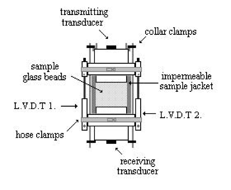
Figure 1: Container and Transducers-LVDT apparatus used in the sound propagation experiments.

Before starting the measurements, a series of tapping and vibrations were applied to the container in order to let the grains settle into the densest possible packing. Our goal is to establish the sample in the reversible state described by, e.g. Figure 2 of Nowak, et al nowak . The entire system was then put into a pressure vessel filled with oil (see Fig. 1). We then applied confining pressures ranging from 0 to 140 MPa. The pressure was cyclically applied several times until the system exhibited minimal hysteresis. At this point shear and compressional waves were propagated by applying pulses. The sound speeds and corresponding moduli were obtained by measuring the arrival time from “head to head” of the transducers for the two sound wave types.

III.2 Acoustic measurements

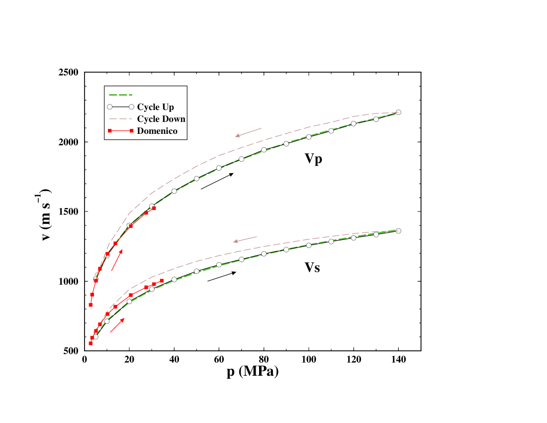
Figure 2: (a) Wave velocities versus pressure obtained in our experiments. Also shown are the results of Domenico domenico for comparison. We cycle up and down in pressure to avoid hysteresis.

The results we obtain are plotted in Fig. 2 and they compare well with the available data of Domenico domenico for the range 0-40 MPa. There remains an hysteresis component between the cycle upwards and downwards in pressure which is representative of the packed system. A more detailed comparison with theory and simulations is done in Figs. (4) and (5), below.

Because of the deformation of the glass beads the height of the system decreases with the increasing pressure. In order to obtain the correct velocities from the arrival time of the signal, we accurately measure the displacement of the transducers as the pressure is increased with a pair of LVDTs. In order to avoid fracture of the particles due to the external pressure we use small particle sizes to reduce the intensity of the contact forces. To get a qualitative idea of the presence of crushing within the system we observe the sample under a microscope after the experiments. We find that crushing occurs only in a very small fraction of the beads. When the experiment was repeated with larger beads of diameter 0.3 mm many particles appeared to be crushed after applying pressures of 140 MPa. Moreover, during this test there was a strong acoustic emission and a severe inflection in the sound speeds could be noticed as we increased the pressure during the first cycle upwards due to the crushing of the beads. For the beads of size $45\mu$m, no inflection is observed and no acoustic emission is heard during the experiment.

IV Numerical simulations

We perform MD simulations of a system of 10000 spherical particles in a periodically repeated cubic cell of approximately 4mm sides. The particles interact via Hertz-Mindlin contact forces and we choose typical values for glass beads for $\mu_{g}=29$ GPa and $\nu_{g}=0.2$ for a close comparison with experiments. We assume a distribution of grain radii in which $R_{1}=0.105$ mm for half the grains and $R_{2}=0.095$ mm for the other half. Our results are quite insensitive to the choice of the size distribution. We include viscous damping terms to allow the system to relax toward static equilibrium as discussed in Section II.5.

The general scheme of the simulations is as follows: The simulations begin with a gas of 10000 grains distributed at random positions inside the cubic cell. We first apply a compression protocol so that a dense random packing is generated corresponding to a predetermined value of the pressure. Then, an incremental infinitesimal compression or shear is applied to the unit cell and the change in stress is computed, once the system re-equilibrates. Thus, we obtain the bulk and shear moduli for the system at each confining pressure.

IV.1 The reference state: numerical protocol

One of the critical issues in this study is how to obtain a proper rigid frame of reference Eq. (9), {R}, from where we could calculate the elastic moduli. Our calculations begin with a numerical protocol designed to mimic the experimental procedure used to prepare dense packed granular materials at a given confining pressure. In the experiments, the initial bead pack is subjected to mechanical tapping and ultrasonic vibration in order to increase the solid phase volume fraction, as discussed in the previous section.

During the numerical preparation stages we turn off the transverse force between the grains ($k_{t}=0$); because there are no transverse forces, the grains slip without resistance and the system reaches the high volume fractions found experimentally during the initial compression process. We found that by preparing the system with frictional and elastic tangential forces, the system reaches states of lower volume fraction. A more complete study of this effect will be presented in Part II unknownauthors . In the following calculation we concentrate on the preparation without friction, so that we can obtain the most compact states possible, mimicking our experimental procedure. We then restore the tangential Mindlin force and friction when we calculate the elastic constants.

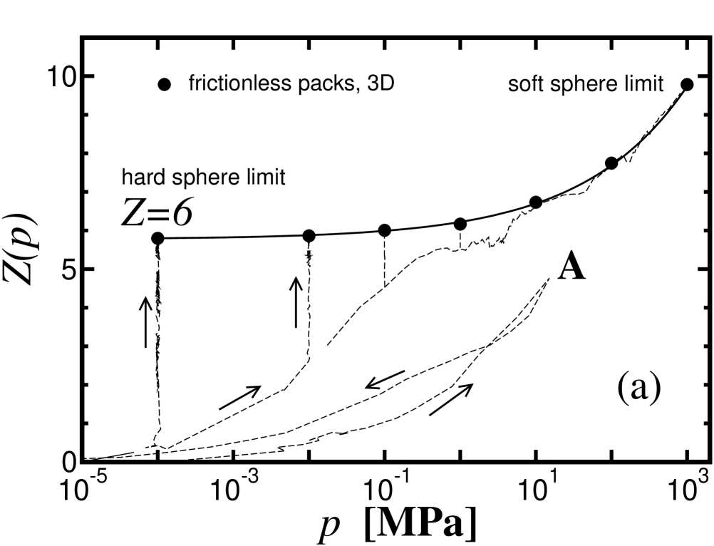
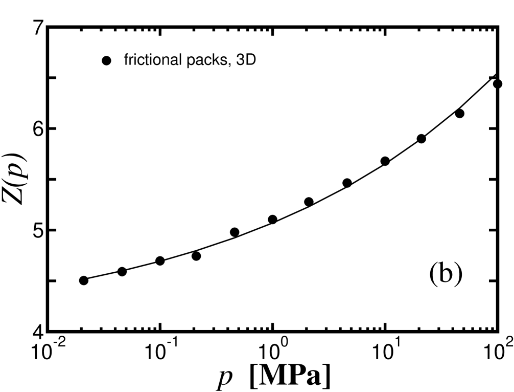
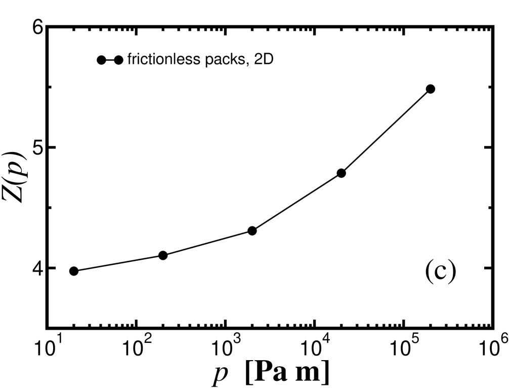
Figure 3: Coordination number versus pressure obtained in the simulations. (a) Frictionless packs in 3D. The system becomes isostatic as $p\to 0$ and $Z\simeq 6$. (b) Frictional packs in 3D. Is the isostatic limit $Z_{c}=4$ reached asymptotically as $p\to 0$? See Part II unknownauthors for details. (c) Frictionless packs in 2D. Here the system is isostatic with $Z_{c}\simeq 4$ as $p\to 0$.

Starting with a set of non-contacting particles, we first apply a slow compression to bring the particles closer until a specified value of the pressure and coordination number is attained. This initial compression is specified by the dashed lines in Fig. 3a. If the compression is stopped just before reaching a volume fraction of random close packing (specified as Point A in Fig. 3a) and the system is allowed to relax, then system will relax to zero pressure and zero coordination number, since it cannot equilibrate below the maximum close packing fraction. This is indicated in Fig. 3a as the decrease of the coordination number and pressure towards zero. The compression is then continued to a point above the critical packing fraction at a target pressure, $p_{t}$. The target pressure, is maintained with a “servo” mechanism cundall which constantly adjusts the applied strain rate $\dot{\epsilon}$ until the system reaches equilibrium at $p_{t}$ according to the following prescription:

$$\dot{\epsilon}=g(p-p_{t}),$$ (28)

where $p$ is the actual pressure of the system and $g$ is a gain factor which is tuned to achieve equilibrium at every given pressure in an optimal way.

IV.2 Coordination number

The above protocol is repeated for different target pressures and we obtain the average coordination number $Z$ of these equilibrium states as a function of the pressure, as seen in Fig. 3a. Several important points can be seen from this plot. Firstly, the average coordination number increases with the pressure as expected. Secondly, we find that the coordination number of the pack approaches a critical minimal value close to $Z_{c}\approx 6$ as $p\to 0$. At low pressures, compared to the shear modulus of the beads ($p\ll 26$GPa), the system behaves more like a pack of rigid balls. At this point the beads are minimally connected at $Z_{c}\approx 6$, while in two dimensions (see Appendix E) the same preparation protocol gives $Z_{c}\approx 4$ (Fig. 3c).

Such low coordination numbers can be understood in terms of simple constraint arguments for a system of $N$ frictionless rigid particles in $D$ dimensions alexander ; isostatic ; edwards-grinev ; ball . We need to determine $ZN/2$ normal forces with $DN$ equations of force balance. We find a critical coordination number for which the equations of force balance are soluble as $Z_{c}=2D$. For large values of the confining pressure more grains are brought into contact, and the coordination number increases from its minimal value required for stability; the system is underconstrained. Empirically, we find in 3D

$$Z(p)=Z_{c}+\left(\frac{p}{~{}\mbox{10 MPa}}\right)^{0.30(5)}.$$ (29)

The pressure 10 MPa is significant since it determines the characteristic pressure of the crossover from the minimal coordination number to a larger one.

We also measure the volume fraction as a function of pressure and find that it approaches a critical value of $\phi_{c}\approx 0.63$ in the rigid ball limit as $p\to 0$:

$$\phi(p)=\phi_{c}+\left(\frac{p}{~{}\mbox{14 GPa}}\right)^{0.62(6)}.$$ (30)

The value of $\phi_{c}=0.63\approx\phi_{\mbox{\scriptsize RCP}}$ corresponds to the volume fraction at random close packing (RCP): the densest possible random packing of hard spheres bernal ; finney ; berryman , since the hard sphere limit in our system of deformable particles is achieved when the pressure (deformation) vanishes (RCP is only achieved asymptotically in our simulations). The exponent 0.62 is consistent with dimensional arguments which would predict a value inverse of the power law between the force and displacement in the Hertz law, i.e. a 2/3 exponent. The exponent in Eq. (29) is determined by the behavior of the pair distribution function near jamming. These exponents agree with similar calculations done by O’Hern et al. ohern , and they will de discussed in more detail in Ref. unknownauthors .

The low value of $Z_{c}$ is very significant (this number should be compared, for instance, to $Z=12$ for a FCC packing) because at this minimal coordination the equations for the force distribution can be solved without reference to the state of strain in the system. This is the isostatic limit alexander ; isostatic and the starting point of recent theories of stress distributions in granular packs edwards-grinev ; fragile ; ball . Concepts such as fragility and marginal rigidity depend on the existence of this minimally connected state. In the conclusions we will come back to discuss this issue. As previously reported in mgjs and makse-fc , Eq. (29) provides a numerical evidence of the existence of the minimally connected state in frictionless granular packs. For other numerical work see silbert .

To test the robustness of these results, we have employed a second protocol in which the system is prepared by compressing to a point beyond the RCP fraction, then letting the grains relax to equilibrium without the servo mechanism. The final $Z(p)$ curve is essentially identical to the one shown in Fig. 3a. For this reason we believe that we have accurately approximated the reversible state of dense random packing, in the sense discussed by Nowak, et al. nowak .

It is important to recall that the above results have been obtained for a system without friction. A similar preparation protocol for grains with friction gives rise to different packings with lower coordination number. Similar constraints arguments as explained above give $Z_{c}=D+1$ for this case. Fig. 3b shows $Z(p)$ obtained for a system with friction showing that a minimal $Z_{c}\approx 4$ in 3D may be approached asymptotically as $p\to 0$, although at a slower rate than in the frictionless case. Is the $Z_{c}=4$ isostatic limit achieved as $p\to 0$? We have given a positive answer to this question in makse-fc . However, recent studies silbert suggest that this may not be the case. We refer the interested reader to Part II of this work unknownauthors for our more recent results showing that the rate of compression (analogous to the rate of cooling of a a glass-forming liquid below the glass transition) plays a significance role in achieving the isostatic limit in frictional packs. From now on we will concentrate on the calculation of the elastic properties of granular media using the states depicted in Fig. 3a as our starting point. Of course, we will restore $k_{t}\neq 0$ for the calculation of the moduli.

IV.3 Calculation of elastic moduli with MD

Consider the calculation of the elastic moduli of the system as a function of pressure. Beginning with the equilibrium states of Fig. 3a we first restore the transverse component of the contact force by setting $k_{t}\neq 0$. We then apply a small perturbation to the system and measure the resulting response. We don’t expect slippage to occur since we apply infinitesimal strain perturbations, but since we deal with a finite system we set the friction coefficient $\mu_{f}$ to a large value to avoid sliding at the contacts. The elastic moduli are calculated by applying a given affine infinitesimal strain perturbation $\Delta\epsilon$ as given by Eq. (10) and then monitoring the response of the corresponding stress $\sigma(t)$ as a function of time. After the system equilibrates again as $t\to\infty$, the moduli are obtained from Eqs. (22) and (24) as the change in stress between the final state and the stress before the perturbation $\Delta\sigma/\Delta\epsilon$. The procedure is repeated for $\Delta\epsilon\to 0$ to guarantee that we are testing the linear response regime where the elastic moduli become independent of $\Delta\epsilon$. Interestingly we find that the region where the elastic constants are well defined decreases as the pressure decreases. This is in agreement with the prediction of the EMT for the 3rd order elastic constants which are found to diverge as $\sim\epsilon^{-1/2}\sim p^{-1/3}$ johnson1 .

The shear modulus is calculated from a simple shear test ($\Delta\epsilon_{12}=\Delta\epsilon_{21}\neq 0$) as given by Eq. (7)

$$\mu=\frac{1}{2}\frac{\Delta\sigma_{12}}{\Delta\epsilon_{12}},$$ (31)

and also from a pure shear test with $\Delta\epsilon_{11}=-\Delta\epsilon_{22}$:

$$\mu=\frac{1}{2}\frac{(\Delta\sigma_{22}-\Delta\sigma_{11})}{(\Delta\epsilon_{22}-\Delta\epsilon_{11})}.$$ (32)

We find that the values of $\mu$ determined from these two methods agree with each other, as expected for an isotropic system.

The bulk modulus is obtained from a uniaxial compression test along the 1-direction and keeping the strain constant in the other directions $\Delta\epsilon_{22}=\Delta\epsilon_{33}=0$, and $\Delta\epsilon_{11}\neq 0$:

$$K=\frac{\Delta\sigma_{11}}{\Delta\epsilon_{11}}-\frac{4}{3}\mu\>\>\>.$$ (33)

Here the stress, $\sigma_{ij}$, is determined from the measured forces on the grains Eq. (27), and the strain, $\epsilon_{ij}$, is determined from the imposed dimensions of the unit cell. For instance $\epsilon_{11}=\Delta L/L_{0}$ where $\Delta L$ is the infinitesimal change in the $11$ direction and $L_{0}$ is the size of the reference state at the given $p$.

The results of our numerical calculations for $K(p)$ and $\mu(p)$ are shown in Fig. 4. These results have been obtained for packings of 10000 particles. Calculations done with 432 spheres show similar values indicating that the results are free of finite size effects. We see that our experimental and numerical results are in reasonably good agreement. Also shown are data measured by Domenico  domenico . Clearly, the experimental data are somewhat scattered at low pressure. It reflects the difficulty of the measurements, especially at the lowest pressures where there is a significant signal loss. Nevertheless, our calculated results pass through the collection of available data. It should be noted that the experiments are compared against the numerical results without resorting to the use of fitting parameters, since all the constants characterizing the grain material ($\mu_{g}$ and $\nu_{g}$) are known from the properties of the grains.

IV.4 Breakdown of the EMT. Problems with $\mu$

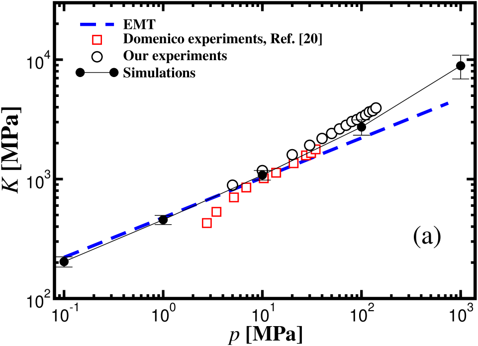
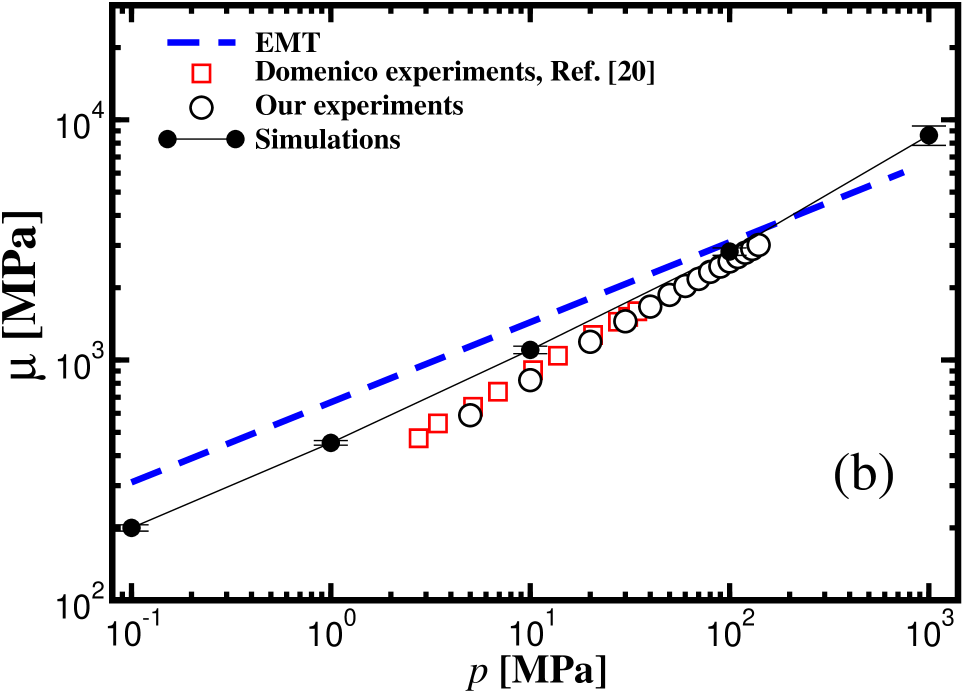
Figure 4: Pressure dependence of the elastic moduli, (a) bulk and (b) shear moduli from MD, our experiments, Domenico experiments and EMT.

Also shown in Fig. 4 are the EMT predictions Eq. (12) and (14) using the same parameters as in the simulations. We set $Z=6$ and $\phi=0.64$, independent of pressure. At low pressures we see that $K$ is well described by EMT. At larger pressures, however, the experimental and numerical values of $K$ grow faster than the $p^{1/3}$ law. The situation with the shear modulus is even less satisfactory. EMT overestimates $\mu(p)$ at low pressures but, again, underestimates the increase in $\mu(p)$ with pressure.

To investigate the failure of EMT in predicting the correct pressure dependence of the moduli, we re-plot the moduli divided by $p^{1/3}$ in Fig. 5.

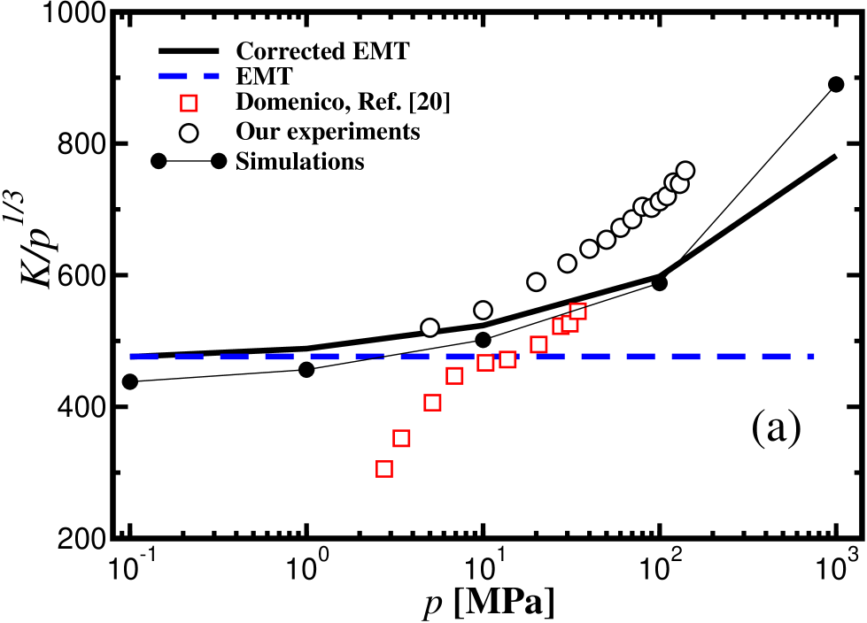
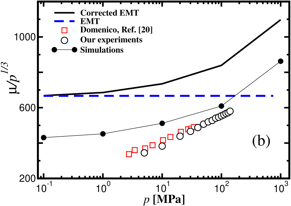
Figure 5: Elastic moduli, (a) bulk and (b) shear, normalized to $p^{1/3}$ and corrected EMT taking into account the pressure dependence of $Z(p)$ from Fig. 3a as well as $\phi(p)$.

For such a plot, EMT predicts a horizontal straight line but we see that the numerical and experimental results are clearly increasing with $p$. It is tempting to try to fit the data with another power law. However, we must first include the power law dependence of the coordination number and the volume fraction with the pressure as given by Eqs. (29) and (30). Thus we modify Eqs. (12) and (14) to include the pressure dependence $Z(p)$ and $\phi(p)$ (this latter is a much smaller effect, see below). The corrected EMT is also plotted in Fig. 5 and we see that it predicts the same trend with pressure as the simulations. The experimental data also seem to be following this trend but more data over a larger pressure range are clearly needed.

When analyzing $K(p)$, we find that the corrected EMT is in essentially exact agreement with our numerical simulations and experimental data. Thus, we tend to conclude that the anomalous scaling found in the experiments is be a measurement of a crossover behavior as obtained by combining Eqs. (12) and (14) with the nonlinearity of Eqs. (29) giving rise to two distinct scaling regimes:

$$K(p) \sim \mu(p)\sim p^{1/3},~{}\mbox{for $p\ll 10$ MPa},$$ (34)

$$K(p) \sim \mu(p)\sim p^{5/9},~{}\mbox{for 10 MPa $\ll p\ll 14$ GPa}.$$

Here we have not included the pressure dependence of the volume fraction Eq. (30) since it appears at the very large pressures above 14 GPa. At these pressures the beads are not supposed to follow anymore the Hertz law (and they may, in fact, fracture). Therefore we exclude this regime from our scaling analysis in Eq. (34).

Since the experiments are usually done near the crossover pressure of 10 MPa, it holds to reason that they could be measuring a crossover behavior rather than a true scaling regime. Moreover, even for pressures larger than 10 MPa the Hertz contact mechanics approach might fail since the Hertz theory is based on small perturbations. Thus, the true final scaling regime Eq. (34) might not be accessible experimentally, at least for glass beads and other rigid materials. It would be interesting to see if such a crossover could be observed in softer materials.

The substitution of Eqs. (29) and (30) into (12) and (14) is something of an ad hoc procedure; Eqs. (12) and (14) were derived under the assumption that $Z$ and $\phi$ are stress-independent quantities. Within the context of the affine assumption, the EMT derivation can be modified to account for a continuously changing coordination number, $Z(p)$. Let us assume that, in the limit of zero pressure, there is a probability distribution $P(h)$ of gap sizes, $h$, between each ball and its neighbors:

$$P(h)=Z_{c}\delta(h)+a_{1}+a_{2}h+...$$ (35)

where $Z_{c}=6$ represents the coordination number at zero stress and the rest is a Taylor’s series expansion around $h=0$. It is straightforward to re-do the derivations leading to Eqs. (12) and (14) following the prescription in, e.g. johnson1 . The results, expressed in terms of the static compressive strain, $\epsilon<0$, are

$$p=\frac{\phi k_{n}}{6\pi}\left[Z_{c}(-\epsilon)^{3/2}+\frac{2}{5}(a_{1}R)(-\epsilon)^{5/2}+...\right]$$ (36)

$$K=\frac{\phi k_{n}}{12\pi}\left[Z_{c}(-\epsilon)^{1/2}+\frac{2}{3}(a_{1}R)(-\epsilon)^{3/2}+...\right]$$ (37)

Using a judiciously chosen value of $a_{1}\neq 0$, and neglecting $a_{2}$ and all higher-order terms, a cross-plot of Eq. (37) against (36) mimics the molecular dynamic simulations in Figure 4. We note, however, that, taken literally, Eq. (35) predicts $Z-Z_{c}\propto p^{2/3}$ for small $p$, in contrast to Eq. (29).

Since the bulk modulus is approximately described by the corrected EMT, throughout the rest of the paper we focus on $\mu(p)$. In Fig. 5 it is shown that even though the pressure trend is well described by the corrected EMT, the theory still overestimates the value of the shear modulus. We will see later that the overestimation depicted in Fig. 5 becomes enormous when the tangential forces are diminished towards zero. In this limit, the breakdown of the EMT is clearly established.

Another way of seeing the breakdown of EMT is to focus on the ratio $K/\mu$, which is independent of pressure in the theory Eq. (17), the simulations, and approximately so in the experiments, as seen in Fig. 6. [The variation at low pressure may reflect the difficulty in propagating sound at low confining pressures]. The experiments give $K/\mu\approx 1.1-1.3$. Our simulations give $K/\mu\approx 1.05\pm 0.05$ in good agreement with experiments. Notice, however, that the EMT predicts $K/\mu=0.71$, as mentioned earlier. Moreover, the effective Poisson ratio from simulations, $\nu\approx 0.27$ is in excellent agreement with that of the experiment $\nu\approx 0.28$, but greatly differs from the theoretical prediction $\nu_{e}=0.02$, Eq. (18).

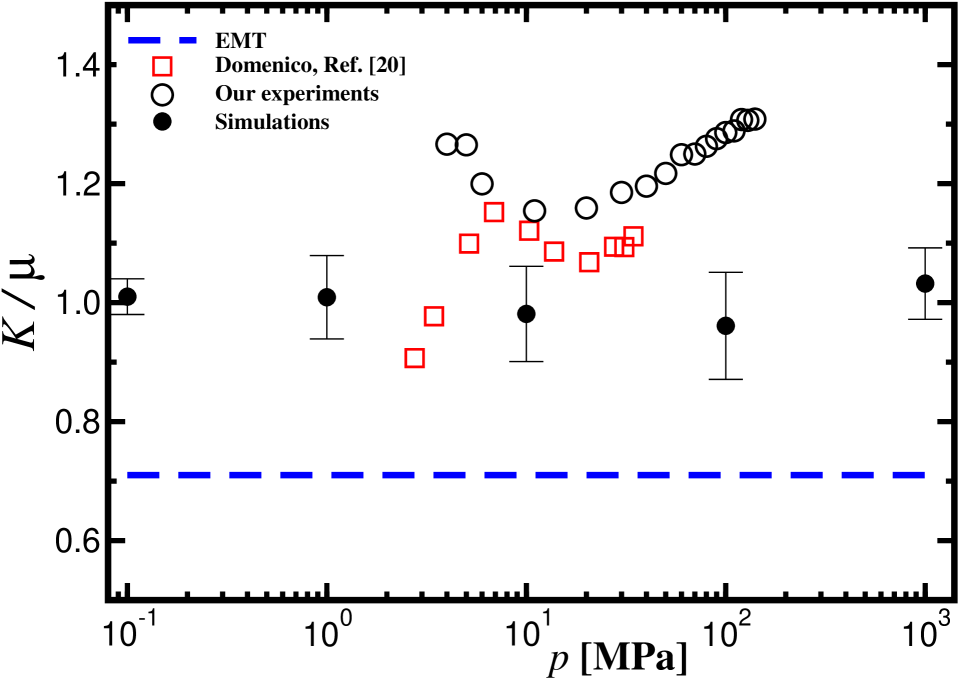
Figure 6: Ratio $K/\mu$ for MD, experiments, and EMT (pressure independent)

IV.5 Role of transverse forces and rotations

To understand why $\mu$ is overestimated by EMT we must examine the role of transverse forces and rotations in the relaxation process of the grains. These effects do not play any role in the calculation of the bulk modulus. According to the EMT, the transverse force $F_{t}$ contributes only to the shear modulus and not to the bulk modulus [see Eqs. (12), (13) and (14)]. We are therefore motivated to examine the behavior of the moduli as a function of the strength of the transverse force. We replace the tangential stiffness $k_{t}$ in Eq. (4) by $\alpha k_{t}$ and redefine the transverse force as

$$\Delta F_{t}=\alpha~{}k_{t}~{}(R\xi)^{1/2}~{}\Delta s,$$ (38)

$\alpha=0$ is appropriate for frictionless coupling (perfect slip), whereas $\alpha=1$ describes the fully frictional result (perfect stick) and corresponds to the results described so far. To quantify the role of the transverse force on the elastic moduli, we calculate $K(\alpha)$ and $\mu(\alpha)$ varying $\alpha$ from 0 to 1, at a given pressure, $p=100$ KPa, low enough so that the changing number of contacts does not play a role.

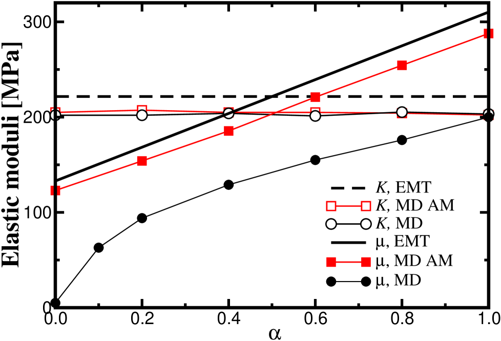
Figure 7: $K(\alpha)$ and $\mu(\alpha)$ versus $\alpha$ for a fixed $p=100$ KPa as calculated numerically with MD (noted MD), as calculated numerically using only the affine motion (noted MD AM) and as predicted by the EMT (noted EMT).

The results are plotted in Fig. 7 (curves labelled MD). To compare with the theory we plot the prediction of the EMT Eqs. (12) and (14) in which $k_{t}$ is rescaled by $\alpha k_{t}$ (curves labelled EMT). (The curves labelled MD AM are discussed in the next subsection.) The simulation confirms that $K$ is essentially independent of the strength of the tangential force; both theory and simulations show a flat line in Fig. 7. Surprisingly, the shear modulus is extremely sensitive to the tangential force and becomes negligible small in the limit of frictionless particles ($\alpha\rightarrow 0$) dropping to less than 10% of the predicted EMT value. We see that the EMT badly fails in accounting for the vanishing of the shear modulus as $\alpha\to 0$. By contrast the bulk modulus agrees reasonably well with EMT regardless of whether there was perfect slip or perfect stick. What is the most serious problem with the elastic theory? In the next section we will focus on the role of stress relaxation and the nonaffine motion of grains due to disorder.

First, however, we wish to eliminate a conceptually simpler effect of disorder as the explanation for the behavior of $\mu(p)$. In the simulations (and presumably in the experiments), it is not true that each grain has the same number of contacts. Rather, there is a distribution of contacts ranging from $Z=3$ to $Z=10$ with a peak at $Z=6$, which is near the average ($\bar{Z}=6.14$ at 100 KPa). Thus, the local elasticity moduli can vary widely from one grain to another. There is a well-developed theory for just such situations bema , which is also called a “self-consistent effective medium approximation” (sc-ema). Let $K_{i}$ and $\mu_{i}$ be the moduli for spherical inclusions whose volume fraction is $c_{i}$. The effective elastic constants for the composite, $K^{*}$ and $\mu^{*}$, are determined by the simultaneous solution of the following coupled equations:

$$\sum_{i}c_{i}\frac{K^{*}-K_{i}}{K_{i}+(4/3)\mu^{*}}=0,$$ (39)

and

$$\sum_{i}c_{i}\frac{\mu^{*}-\mu_{i}}{\mu_{i}+F^{*}}=0,$$ (40)

where

$$F^{*}=\frac{\mu^{*}(9K^{*}+8\mu^{*})}{6(K^{*}+2\mu^{*})}\>\>\>.$$ (41)

Effective medium theories of this sort generally work well in situations in which the disorder is not too great (such as when there is a log-normal distribution of constituent properties, or when one is near a percolation threshold). Moreover, the sc-ema have certain desired properties, such as correct limiting values and lying within upper and lower bounds. See bema for details.

Here we take the view that the system is a composite consisting of spherical inclusions, each of which has moduli given by Eqs. (12) and (14). In the case at hand it is useful to rewrite them in terms of the local value of the compressive strain, $\epsilon_{i}<0$, within each inclusion [See Ref. johnson1 for details]:

$$K_{i}=\frac{\phi k_{n}}{12\pi}Z_{i}(-\epsilon_{i})^{\frac{3}{2}},$$ (42)

$$\mu_{i}=\frac{\phi(k_{n}+\frac{3}{2}\alpha k_{t})}{20\pi}Z_{i}(-\epsilon_{i})^{\frac{3}{2}}.$$ (43)

Of course, grains with a large number of contacts, $Z_{i}$, can be expected to have a smaller than average compressive strain, $\epsilon_{i}$. In order to relate $\epsilon_{i}$ to the macroscopic strain, $\epsilon^{*}$, we recognize that the spirit of the sc-ema is that each spherical inclusion is surrounded by the host material. Therefore, it is a simple elasticity problem to show that the differential change in strain within a spherical inclusion is related to the differential change in macroscopic strain by

$$d\epsilon_{i}=\frac{K^{*}+(4/3)\mu^{*}}{K_{i}+(4/3)\mu^{*}}d\epsilon^{*}\>\>\>.$$ (44)

We take the distribution of contacts $\{c_{i}\}$ from our simulation at 100 KPa. It is straightforward to solve the system of equations (39)-(44). The EMT we have been discussing corresponds to $Z_{i}\rightarrow<Z>$ and $\epsilon_{i}\rightarrow\epsilon^{*}$; for the case $\alpha=0$, and using the same material parameters as before, it may be written as

$$K_{e}=16.2(-\epsilon^{*})^{3/2},$$ (45)

$$\mu_{e}=9.7(-\epsilon^{*})^{3/2},$$ (46)

where the moduli are expressed in GPa. If, though, the full distribution of contact numbers is used in the foregoing analysis the results are

$$K^{*}=15.8(-\epsilon^{*})^{3/2},$$ (47)

$$\mu^{*}=9.5(-\epsilon^{*})^{3/2}\>\>\>.$$ (48)

The point of this exercise is to demonstrate that, although the packing is obviously disordered, the effect of the disorder alone is quite negligible as far as the macroscopic elastic moduli are concerned. Similar results hold for $\alpha=1$. Each grain sees, more-or-less, the same average environment as any other. In the next section we investigate the effects of disorder induced relaxation, which, we believe is the underlying effect behind the small values of $\mu(p)$ we are observing.

IV.6 Role of relaxation and disorder

In the EMT, we saw that if an affine perturbation of the form (10) is applied to the system, the grains are always at equilibrium due to the assumption of isotropic distribution of contacts and further relaxation of the grain is not significant. The response is then purely elastic.

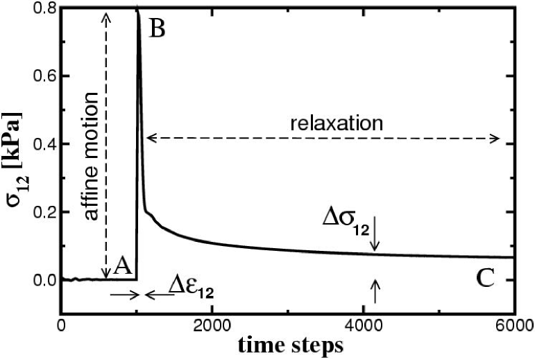
Figure 8: Relaxation of the shear stress (B$\to$C) after an affine motion (A$\to$B) in the calculation of the shear modulus.

On the contrary, in the MD simulations (and in the experiments) after the application of an affine perturbation via the motion of the boundaries and grains, the beads in the immediate neighborhood of each grain move around, relative to the center grain, in a way which gives rise to a stress relaxation associated with these rearrangements of particles.

Figure 8 shows the behavior of $\sigma_{12}(t)\equiv\epsilon_{12}G(t)$ as per Eq. (20) for a system at $p=100$ KPa and with $\alpha=0.2$ during and after the application of the affine strain perturbation $\Delta\epsilon_{12}$ which moves all the grains according to the external strain Eq. (10). We see how the system behaves as a viscoelastic solid as explained in Section II.4. When the affine perturbation is applied, the shear stress increases (from A to B in Fig. 8) and the grains are far from equilibrium since the system is disordered. This is the instantaneous elastic response. The grains then relax towards equilibrium as (from B to C), and we measure the resulting change in stress $\Delta\sigma_{12}$ as $t\to\infty$ from which the modulus $\mu$ is calculated as in Eq. (22).

For a better understanding of the approximations involved in the EMT, suppose we repeat the MD calculations now taking into account only the affine motion of the grains and ignoring the subsequent relaxation. The resulting values of the moduli are obtained as $\mu_{\mbox{\scriptsize affine}}=\Delta\sigma_{12}^{\mbox{\scriptsize affine}}/\Delta\epsilon_{12}$ with $\Delta\sigma_{12}^{\mbox{\scriptsize affine}}$ defined in Fig. 8. In Fig. 7 we plot the moduli calculated in this way as a function of $\alpha$ for $p=100$ KPa (curves labelled MD AM). The affine moduli are very close to the EMT predictions: there remains a 10% difference between the EMT and the MD (affine) which is representative of the disordered packing which is averaged in the EMT. Thus, the difference between the MD and EMT results for the shear modulus lies mostly in the non-affine relaxation of the grains; this difference is largest when there is no transverse force.

By contrast, grain relaxation after an applied compressional affine perturbation is not particularly significant and the EMT predictions for the bulk modulus are quite accurate as seen in Fig. 7.

IV.7 The isostatic limit as a critical point

The surprisingly small values we found for $\mu$ as $\alpha\rightarrow 0$ raises several questions. We notice that $k_{n}$ and $p$ are the only variables with the dimension of pressure in this limit. A scaling argument would lead to

$$\mu\sim k_{n}(p/k_{n})^{\eta}.$$ (49)

The Hertz theory predicts $\eta=1/3$, a result which we find to be valid at low pressure for frictional grains. Indeed, quite generally if one assumes that each grain-grain force scales as Eqs. (3) and (4) and if one assumes the arrangement of the grains, however disordered that may be, does not change with pressure then both moduli scale as in Eq. (49) with $\eta=1/3$. This argument specifically presupposes that e.g. the average coordination number does not change with pressure.

Since there are no other constants that could reduce the value of $\mu$ for $\alpha\rightarrow 0$ we are lead to believe that a new exponent $\eta$ should describe the shear modulus for frictionless packs. This is an effect which lies outside the standard assumptions of elasticity theory, as indicated above. Since $p<k_{n}$, then $\eta>1/3$. To give validity to our hypothesis, we plot in Fig. 9 $\mu(p)$ for $\alpha=1$ and $\alpha=0$. We see that a better fit to the low pressure behavior of $\mu(p)$ for $\alpha=0$ is achieved with $\eta=2/3$. Notice that we deliberately try to fit the data at low pressure to avoid the issue of the increasing coordination number.

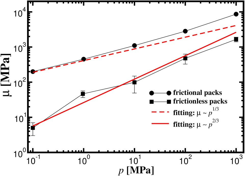
Figure 9: Shear modulus versus pressure for frictional ($\alpha=1$) and frictionless ($\alpha=0$) particles.

How can we explain the $2/3$ scaling behavior? A possible answer could be provided by a recent conjecture by Alexander alexander who proposed the following scaling

$$\mu\sim k_{n}{\cal A}(p)(p/k_{n})^{\eta}.$$ (50)

where the function ${\cal A}(p)$ is determined by the geometry of the reference frame of rigidity, Eq. (9), which is determined, in turn, by the pressure. Assuming that the limit $p\to 0$ is indeed a critical state of rigidity, then we expect

$${\cal A}(p)\sim p^{\lambda},$$ (51)

which would explain the anomalous scaling for the frictionless grains with $\lambda=1/3$, while for frictional grains we would have $\lambda=0$.

IV.8 Microstructure and force chains.

The velocity of acoustic signals probes an effective medium which should be homogeneous at length scales larger than a typical correlation length of the material. Experimental and numerical work indicates that there is an internal structure at length scales $\sim 10d$, where $d$ is the typical size of the grains: the forces are observed to be localized along “force chains” carrying most of the loads in the system (see Fig. 11) makse-fc ; fc3 ; cundall2 ; chicago1 . A question of interest is how such a microstructure affects the properties of the system at macroscopic length scales where the elastic continuum theory is valid jussieu .

We want to quantify the relevance of force chains to the elastic moduli. We calculate the shear modulus as a function of a subset of forces belonging to the strongest forces in order to search for the backbone of grains which give rise to the shear rigidity of the material. Is this backbone determined by the force chains, or do the interstitial particles play also a relevant role to determine the rigidity?

In this regard, recent calculations of Radjai et al. radjai2 have shown that the stress ratio between shear and compression shows a “percolation-like” behavior: the forces larger than the average are responsible for most of the rigidity of the material. This was shown to be valid in 2D. Here we follow radjai2 and define a $\zeta$-network which includes only forces smaller than a cutoff force $\zeta$. Then we redefine the stress Eq. (27) and compute the shear stress only for the $\zeta$-network as

$$\sigma_{12}(\zeta)=\frac{1}{2V}\sum_{|\mbox{\bf F}|<\zeta}(F_{i}Rn_{j}+Rn_{i}F_{j}),$$ (52)

from which we obtain the shear modulus for the $\zeta$-network as $\mu(\zeta)=\Delta\sigma_{12}(\zeta)/\Delta\epsilon_{12}$ (for $\zeta\to\infty$ we recover our previous results).

Figure 10 shows the result of $\mu(\zeta)$ for $p=100$ KPa and $\alpha=1$ and should be compared with Fig. 4 in radjai2 . In contrast with the 2D results of radjai2 we find no evidence of a bimodal distribution of forces which would give rise to a percolation-like behavior of the shear modulus. We see that the shear modulus and the coordination number increase continuously as we increase $\zeta$.

We also repeat the same calculations for our two-dimensional packings and find the same result as in 3D, i.e. we find no evidence of a bimodal character in the behavior of the shear modulus versus the force cut-off. The fact that we do not see the same behavior in 2D as in radjai2 might be related to the regularization scheme used in our MD simulations to handle the frictional forces which may eliminate the critical behavior found in radjai2 . Radjai et al. used a Contact Dynamics algorithm which tackle the non-smooth character of the interactions without any regularization schemes.

Figure 11 shows our attempt to visualize force chains in 3D packings (a) without friction under isotropic compression, (b) with friction under uniaxial compression and (c) in 2D frictional isotropic packings. Force chains are not prominent in the 3D isotropic frictionless packing. Moreover, the continuous variation of $\mu(\zeta)$ obtained for this packing seems to indicate that all forces are important for the mechanical response to shear, and not just the larger forces which may be organized in force chains. However, force chains are prominent in the 3D packing under uniaxial compression and the 2D packing.

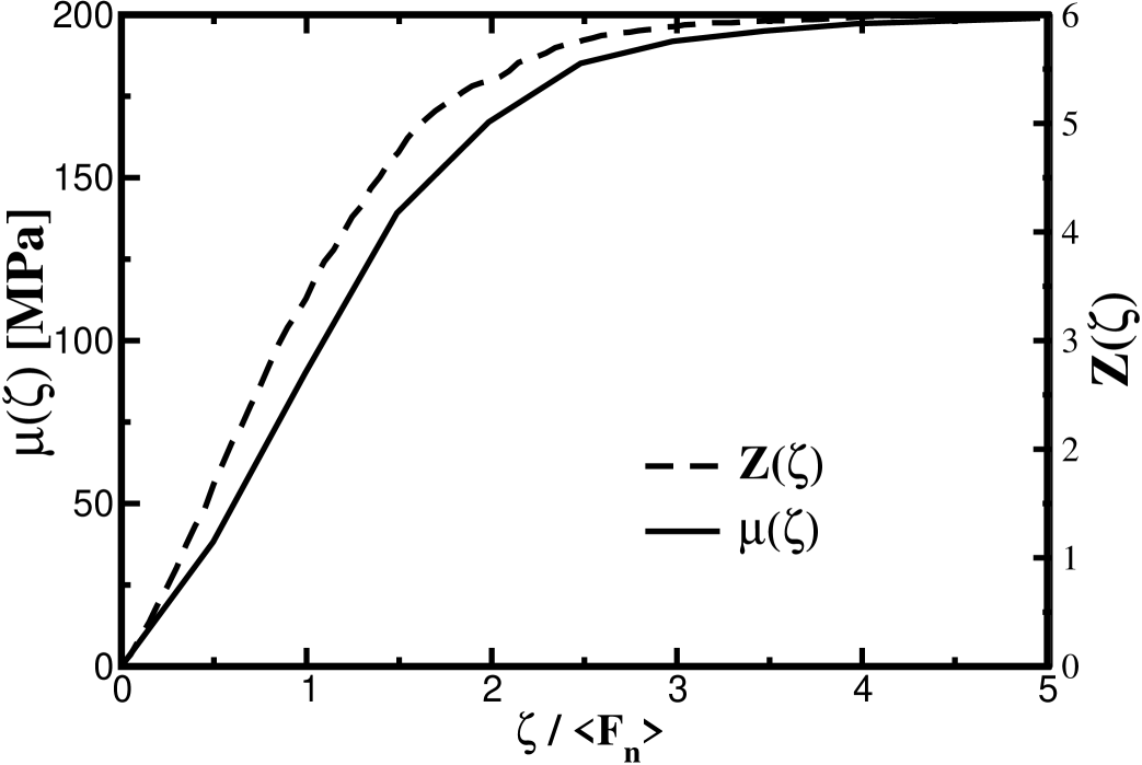
Figure 10: Behavior of the shear modulus and the coordination number for the $\zeta$-network. We use the packing at 100 KPa depicted in Fig. 11a for this calculation.

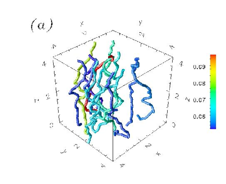
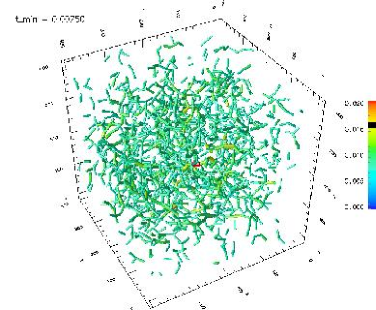
(a) (b) (c)

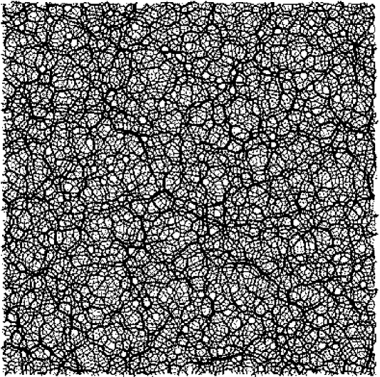
Figure 11: (Color online) Force chains in granular matter: (a) Frictional system under uniaxial compression near $\phi_{c}$ (from makse-fc ). Percolating force chains are seen in this case. We apply an algorithm which looks for force chains by starting from a sphere at the top of the system, and following the path of maximum contact force at every grain. We plot only the paths which percolate, i.e., stress paths spanning the sample from the top to the bottom. (b) Frictionless isotropic system at $p=100$ KPa in 3D. We plot only the forces larger than the average. Force chains seem to be tenuous and not well defined. (c) Force chains in a 2D frictional system. Force chains are clear in this case.

V Theory: single particle relaxation

Since the difficulty with the shear modulus is shown to be due to the relaxation of the particles from the initial uniform strain approximation, we next perform the simplest investigation that allows for some relaxation. From the simulations, we know the rest positions of each of the particles, as well as the contact vectors $\hat{\bf d}^{(q)}=({\bf x}_{1}-{\bf x}_{2})/|{\bf x}_{1}-{\bf x}_{2}|$ (the vector from a particle to each of the particles with which it is in contact). Consider a specific particle. We make the approximation that when a small amplitude macroscopic strain is applied its contacting particles move according to the affine approximation. The particle will experience an unbalanced force and an unbalanced torque. Accordingly, it will relax to a new position and orientation such that the net force and torque on it become zero. So, for the specific particle we calculate its new position and orientation. We next calculate the energy stored within each of the contact “springs”. We do this for each of the particles in the simulation to calculate the total stored energy due to the applied strain and we set this equal to the usual expression for strain energy in order to deduce the new estimates for the bulk and shear moduli of the aggregate. This procedure is detailed below.

Consider a particle, labeled $a$, which we take to be centered at the origin. It has $z_{a}$ contacts at the positions $\{{\bf d}^{(q)}:q=1,z_{a}\}$. Assuming that one of the contact points is displaced by an amount ${\bf u}^{(q)}$ the increment in the intergrain force at contact $q$ is

$${\bf F}^{(q)}_{u}=K_{N}[(\hat{\bf d}^{(q)}\hat{\bf d}^{(q)})\cdot{\bf u}^{(q)}]+\alpha K_{T}[({\bf I}-\hat{\bf d}^{(q)}\hat{\bf d}^{(q)})\cdot{\bf u}^{(q)}],$$ (53)

where $K_{N}$ and $K_{T}$ are given by:

$$K_{N}=\frac{2\mu_{g}R^{1/2}}{1-\nu_{g}}\xi^{1/2},$$ (54)

$$K_{T}=\frac{4\mu_{g}R^{1/2}}{2-\nu_{g}}\xi^{1/2},$$ (55)

and $\xi$ is the normal displacement which can be related to the external pressure through the average affine approximation walton by

$$\xi=R\left[\frac{3\pi}{2}\frac{(1-\nu_{g})}{\phi Z}\frac{p}{\mu_{g}}\right]^{2/3}.$$ (56)

The parameter $\alpha$ allows us to continuously investigate the crossover behavior from perfect slip ($\alpha=0$) to perfect stick ($\alpha=1$).

As written, the total force on the specific particle, due to the sum of all the contact forces is not zero:

$${\bf F}_{u}\stackrel{{\scriptstyle def}}{{=}}\sum_{q}{\bf F}^{(q)}_{u}\neq 0\>\>\>.$$ (57)

Accordingly, that particle will move to a new equilibrium position, ${\bf X}$. Similarly, the net torque on the particle is unbalanced:

$${\bf N}_{u}\stackrel{{\scriptstyle def}}{{=}}\sum_{q}{\bf d}^{(q)}\times{\bf F}^{(q)}_{u}\neq 0.$$ (58)

Accordingly, the particle will rotate through an angle $\omega$ to a new orientation. The generalization of Eq. (53) that takes into account the new position and orientation is

$$\begin{array}[]{ll}{\bf F}^{(q)}=&K_{N}[(\hat{\bf d}^{(q)}\hat{\bf d}^{(q)})\cdot({\bf u}^{(q)}-{\bf X})]+\\ &\alpha K_{T}[({\bf I}-\hat{\bf d}^{(q)}\hat{\bf d}^{(q)})\cdot({\bf u}^{(q)}-{\bf X})-\mbox{\boldmath{$\omega$}}\times{\bf d}^{(q)}],\end{array}$$ (59)

Now, the requirement that the particle is in equilibrium with its contact forces, $\sum_{q}{\bf F}^{(q)}\stackrel{{\scriptstyle set}}{{=}}0$, gives three linear equations in the six unknowns, $\omega$ and ${\bf X}$. The requirement that the total torque must vanish, $\sum_{q}{\bf d}^{(q)}\times{\bf F}^{(q)}\stackrel{{\scriptstyle set}}{{=}}0$, gives the remaining three. It is straightforward to solve these equations numerically.

Having determined the new equilibrium position and orientation, one can show that the total work done by the contact forces on the $a$-th particle is simply

$$\begin{array}[]{ll}W_{a}=&\frac{1}{2}\{K_{N}\sum_{q=1}^{z_{a}}(\hat{\bf d}^{(q)}\cdot{\bf u}^{(q)})^{2}+\\ &\alpha K_{T}\sum_{q=1}^{z_{a}}\mid\hat{\bf d}^{(q)}\times{\bf u}^{(q)}\mid^{2}-{\bf F}_{u}\cdot{\bf X}-{\bf N}_{u}\cdot\mbox{\boldmath{$\omega$}}\},\end{array}$$ (60)

$\bf{X}$ and $\omega$ are determined as described above. In order to calculate $W_{a}$ we make the affine assumption, that the displacement at the contact point is simply related to the macroscopic strain by Eq. (10). Since we know the exact positions of each contact vector, ${\bf d}^{q}$, from the simulations, we are able to evaluate Eq. (60) for each particle in the ensemble.

We now evaluate $\sum_{a}W_{a}/V$ for a pure compression and for a simple shear numerically and we equate the result to the elastic energy, Eq. (6), in order to deduce the values of $K$ and $\mu$.

The above procedure can only reduce the moduli relative to those of the effective medium prediction. If, in Eq. (60), we assume there is no relaxation [$\mbox{\boldmath{$\omega$}}=0$ and $\bf{X}=0$], and if we replace the sum over contacts by an integral over a presumed uniform distribution of contact directions, we reproduce the effective medium theory, Eqs. (12) and (14).

The results of such a calculation are shown in Fig. 12, which is to be compared to Fig. 7. The static confining pressure is 100 KPa. We see that, relative to the effective medium prediction, there is a small reduction of the bulk modulus, which is relatively insensitive to $\alpha$. There is a much larger reduction of the shear modulus but the results of the simulations for the shear modulus give values that are even smaller still. For $\alpha=0$ (perfect slip) the simulations give $\mu=8\pm\>3$ MPa, which is essentially indistinguishable from zero, whereas from Figure 12 we have a value of 100 MPa. We see that relaxation effects at the single particle level, while significant, are by no means sufficient to explain the effect. In the fully frictional case of $\alpha=1$ there is a reduction relative to the EMT but the simulation gives a value of $200\pm\>10$ MPa. (In Fig. (12) we have extended the calculations into the unphysical range of $\alpha>1$ to emphasize that there is a slight change of slope, relative to the EMT.)

We are thus lead to consider a more sophisticated theory in which we explicitly account for collective fluctuations. The next step in this direction is developed in laragione where we introduce fluctuations in pairs of contacting particles. This theory is developed for the frictionless case, where the reduction in shear modulus is most dramatic and for which we can derive an analytic result using some fairly weak assumptions.

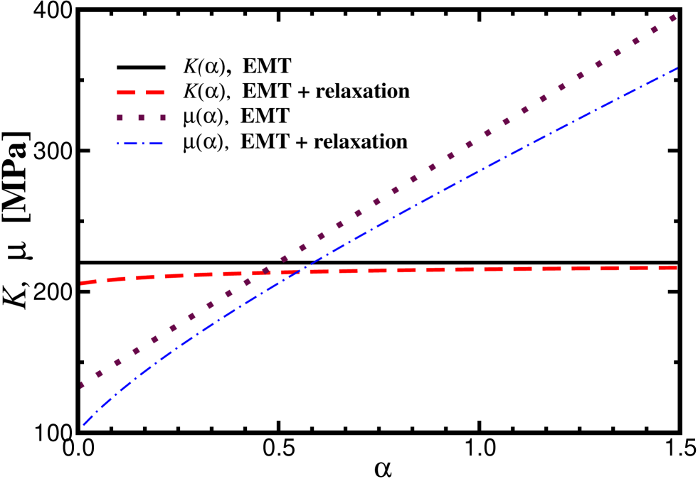
Figure 12: First order correction to EMT allowing relaxation of grains from the affine motion. This figure should be compared with Fig. 7.

VI Summary and outlook

Where do we go from here? We clearly need new theoretical frameworks to describe the collective relaxation of granular materials, especially under shear and for frictionless packs. Below we give a short review of some of the ideas that have been proposed recently, and how these theories are related to our results.

VI.1 Elastic versus fragile matter

We have seen that the impossibility of defining a strain field which is inhomogeneous at the level of the grain is at the root of the problems of the elastic theory: the EMT approach relies on the assumption of a uniform strain field at all scales landau ; green3 .

Interestingly, recent studies edwards-grinev ; fragile ; ball have proposed theories of stress transmission in granular packs which describe the internal stresses without resorting to the use of strain variables, as in elasticity theory. These groups argue that cohesionless grains are in a “fragile state” of marginal rigidity or isostatic at a minimal coordination number $Z_{c}$ and they are only able to support certain loads without severe rearrangements. A novel closure relation between stress components— for instance, the fixed principal axis ansatz— and not between stress and strain— as in elasticity— has been proposed to solve for the indeterminacy in the granular system fragile .

The correct type of closure relation (elastic or fragile) is still a question of much debate savage-elastic , although there are recent experiments on the single-particle Green function measurements suggesting that the elastic framework might be the correct approach at large scales green1 ; green2 ; green3 .

In the case of collective relaxation dynamics, our results show that the elastic formulation is erroneous in describing the macroscopic shear response of granular materials. Moreover, we find that a very small shear modulus appears for frictionless packs. This shear modulus decreases towards zero as $p\to 0$, as $\phi\to\phi_{\mbox{\scriptsize RCP}}$, and as the system approaches the isostatic limit of $Z\to Z_{c}=6$.

The vanishing of the shear modulus could be interpreted as a “fragile” behavior. In the limit $\alpha\to 0$ a packing of nearly rigid particles responds to an external isotropic load with an elastic deformation and a finite $K$, since the external perturbation is compatible with the principal axes of the stress predetermined by the preparation history of the sample. By contrast, such a system cannot support a shear load ($\mu\to 0$) without severe particle rearrangements. Thus the granular system supports, elastically, only perturbations compatible with the structure of force chains and deform irreversibly otherwise, i.e. it is in a “fragile” state.

VI.2 Jamming and melting

Our results show that the fragile limit is approached as the system gets closer to RCP limit, and that at RCP there is a jamming transition between a liquid-like state and a solid-like state with a finite modulus. The approach to the critical point is characterized by several power-law exponents as in a second-order phase transition. The vanishing of the shear modulus can be understood as a melting of the system occurring when the system approaches the isostatic point. This fluid like behavior has similarities with melting transitions found in compressed emulsions, and foams lacasse ; durian ; bolton near the RCP fraction. A slow relaxation time and the increase of the correlation length between force chains is found near RCP. This behavior indicates that the physics of granular materials might be closely related to other complex systems undergoing jamming as proposed recently liu such as glasses, colloids, foams, and emulsions.

VI.3 Conclusions

Our MD simulations are in good agreement with the available experimental data on the pressure dependence of the elastic moduli of granular packings. They also serve to clarify the deficiencies of EMT. Grain relaxation after an infinitesimal affine strain transformation is an essential component of the shear (but not the bulk) modulus. This relaxation is not taken into account in the EMT.

Clearly, there is a need for alternative theories to describe granular packings. Recent work on stress transmission in minimally connected networks may provide an alternative formulation and allow a proper description of the response of granular materials to external perturbations.

Acknowledgments: This work was supported by the DOE, Chemical Sciences, Geosciences and Biosciences Division, and the NSF, Division of Materials Research.

VII Appendix

Appendix A: Resistance against rolling and tangential force with microslip

Our model of the intergrain contact is based on two assumptions. First, we consider the no-slip solution of Mindlin for the tangential force, and we consider total slip of the contact area only when the total tangential force exceed $\mu_{f}F_{n}$. However, in reality, the contact may slip over an annular ring of the contact area for any finite value of the tangential force. A general study for several loading histories considering that microslip occurs, i.e., $|\Delta F_{t}|>\mu_{f}\Delta F_{n}$, was performed by Mindlin-Deresiewicz dere and analyzed in more detail by Thornton and Randall randall . They showed that the incremental tangential force can be obtained as: $\Delta F_{t}=\varepsilon k_{t}(R\xi)^{1/2}\Delta s\pm\mu_{f}(1-\varepsilon)\Delta F_{n},$ where $\varepsilon=1$ when microslip does not occur ($|\Delta F_{t}|<\mu_{f}\Delta F_{n}$) and $\varepsilon$ takes different values depending on the path loading history of loading, unloading and reloading randall . We have done preliminary tests using this more general solution of the tangential force, and found no significant changes in comparison with the results obtained with the no-slip solution of Mindlin. Therefore, we have performed our simulations using the simpler Mindlin contact theory. Besides, the EMT calculations are done using Hertz-Mindlin forces, so that we want to use the same interparticle laws for a better comparison between numerics and theory.

Second, while rotation of spherical grains is allowed in the simulations, it is customary to model rotations without resistance against rolling at the contacts cundall . Regarding this approximation, it should be pointed out that some recent studies oda showed that resistance against rolling (modeled as an elastic spring yielding rotational resistance $k_{r}\theta_{r}$, where $k_{r}$ is the rotational stiffness, and $\theta_{r}$ is the relative rotation by rolling) might be relevant for modeling shear bands. The relevancy of rotational resistance to static packings has not been determined yet, and therefore, we do not include it in our studies. It should be noted, however, that the simulations consider resistance against shear given by the elastic tangential force of Mindlin.

Appendix B: Damping

Recently it has been shown that in order to incorporate the dissipation law leading to inelasticity at the grain-grain contact consistent with the Hertz contact law, a nonlinear force dependency on the relative velocity of the grains in contact has to be incorporated into the contact law poschel2 .

This dissipative part of the normal force has been determined recently by Brilliantov et al. poschel2 as:

$$F_{n}^{diss}=\frac{2}{3}~{}Ak_{n}R^{1/2}\xi^{1/2}\dot{\xi}\>\>\>,$$ (B.1)

where $A$ is a relaxation time that depends on the viscous properties of the grain material, and it can be uniquely determined from experimental measurements of the coefficient of restitution for spherical beads wolf-md ; resti ; bridges .

In our studies, we are not interested in the way the system approaches the equilibrium state, but only in the final state which is supposed to be independent on the type of damping used. Thus, we use the more efficient global damping and linear contact damping described in Section II.5. However, for dynamical studies a damping term as in Eq. (B.1) should be considered as well.

Appendix C: Model of interaction between droplets

In the case of emulsions, interdroplet forces are not given in terms of bulk elasticity as in Hertz theory. Instead, forces are given by the principles of interfacial mechanics without considering shear forces lacasse ; durian ; faraday ; Princen1983 . For small deformations with respect to the droplet surface area, the energy of the applied stress is presumed to be stored in the deformation of the surface. Hence, at the microscopic level, two spherical droplets in contact interact with a normal repulsive force $F_{n}\sim R\gamma A$. This is the so-called Princen model Princen1983 , where $A$ is the area of deformation, and $\gamma$ is the interfacial tension of the droplets, and $R$ is the geometric mean of the radii of the undeformed droplets. Since the area of deformation is proportional to overlap $\xi$, then the interdroplet interaction is $F_{n}\sim\gamma\xi$.

There have been more detailed numerical simulations lacasse to improve on this model and allow for anharmonicity in the droplet response by also taking into consideration the number of contacts by which the droplet is confined. Typically these improved models lead to a force law for small deformations of the form $F_{n}\propto A^{b}$ , where $A$ is the area of deformation and $b$ is a coordination number dependent exponent ranging from 1 (Princen model) to 3/2 (Hertz model) (see also unknownauthors ).

Appendix D: Time step

The time step is usually chosen much smaller than the collision time. However, since each contact is enduring, the collision time is extremely large and other conditions must be used. Besides, the collision time for Hertz spheres depends on the relative velocities of the particle, thus it does not defined a fixed time scale landau .

We choose the time step to be a fraction of the time that it takes for a sound wave to propagate on the grain. Moreover, the quasi-static approximation used to calculate the Hertz force is valid only when the relative velocities of the particles is smaller than the speed of sound in the grains poschel2 . Thus, the characteristic time is $t_{0}=R\sqrt{\rho_{g}/\mu_{g}}$. Typically, one chooses a time interval much smaller than the characteristic time, then $\Delta t=aR\sqrt{\rho_{g}/\mu_{g}}$ with $a<1$. Typical values for glass beads are: $\rho=2600$ Kg/m³, $\mu_{g}\approx 29$ GPa, $R=0.1$ mm. Then $\Delta t$ should be smaller than $10^{-8}$ s. Thus, in order to perform a simulation over one second, more than $10^{8}$ MD steps are needed, which is obviously a very intensive computation. In this case, it is customary to increase the density or decrease the rigidity of the particles to allow for a larger time step to integrate the equations of motion over realistic periods of time. If the shear modulus of the grains in decreased, then it should be checked that the resulting stresses are several order of magnitude smaller than $\mu_{g}$, thus ensuring the condition of a nearly rigid system even though $\mu_{g}$ is taken smaller to obtain larger time steps.

Appendix E: Results in 2D

Here we show the results for the bulk and shear modulus as a function of the pressure for a two-dimensional pack of spherical particles interacting via Hertz-Mindlin forces. The 2D simulations are done with spherical Hertz-Mindlin balls constraint to move in a plane. Thus the interparticle force is that of the 3D case. Our system is not the same as a packing of disks in 2D since the latter has a different interaction law between particles. Our results are analogous to the three-dimensional case shown in Fig. 5. All the conclusions regarding the moduli obtained for 3D are valid in this case as well.

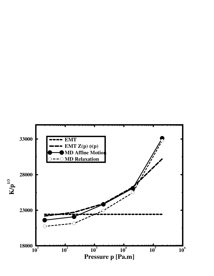
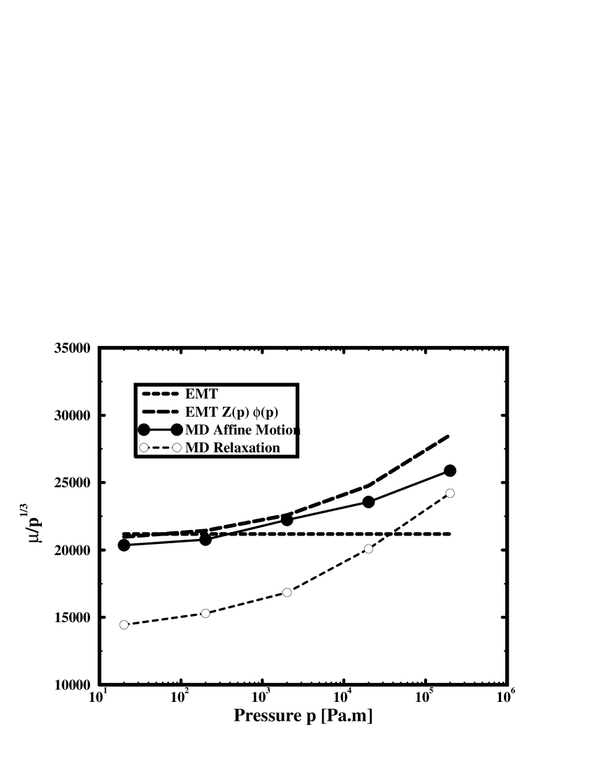
Figure 13: Bulk and shear moduli for a 2D packing normalized to $p^{1/3}$, EMT and corrected EMT taking into account the pressure dependence of $Z(p)$ from Fig. 3c as well as $\phi(p)$ (see Eqs. (D.2) and (D.3).

The scaling of the coordination number is similar to the 3D case:

$$Z(p)=Z_{c}+\left(\frac{p}{~{}\mbox{18 KPa m}}\right)^{0.28(7)},$$ (D.2)

with $Z_{c}\approx 4$.

For the volume fraction we obtain

$$\phi(p)=\phi_{c}+\left(\frac{p}{~{}\mbox{32 MPa m}}\right)^{0.4(1)}.$$ (D.3)

with a critical value of $\phi_{c}\approx 0.835$, which is the RCP limit in 2D. This latter exponent is in disagreement with a mean field prediction based on the contact law, which would imply an exponent 2/3 [see discussion after Eq. (30)]. However, we notice the large error bar of this result since we have only five data points. We refer to unknownauthors for a more systematic study of this problem.

References

- (1) R. P. Behringer and J. T. Jenkins, eds., Powders & Grains 97 (Balkema, Rotterdam, 1997).
- (2) J. D. Goddard, “Nonlinear Elasticity and Pressure-dependent Wave Speeds in Granular Materials”, Proc. R. Soc. Lond. A 430, 105 (1990).
- (3) R. A. Guyer and P. A. Johnson, “Nonlinear Mesoscopic Elasticity: Evidence for a New Class of Materials”, Phys. Today, 52, 30 (1999).
- (4) H. J. Herrmann, J. P. Hovi, and S. Luding, eds., Physics of Dry Granular Matter (Kluwer, Dordrecht, 1998).
- (5) B. K. Sinha, M. R. Kane, and B. Frignet, “Dipole Dispersion Crossover and Sonic Logs in a Limestone Reservoir”, Geophysics 65, 390 (2000).
- (6) In this study, nonlinear effects refer to the fact that the elastic moduli— calculated using small-amplitude strains— depend nonlinearly on the external stress, and they do not refer to the nonlinear mechanical response to large strain perturbations.
- (7) K. L. Johnson, Contact Mechanics, (Cambridge University Press, Cambridge, 1985).
- (8) L. D. Landau and E. M. Lifshitz, Theory of Elasticity (Pergamon, NY, 1970).
- (9) J. Duffy, and R. D. Mindlin, “Stress-Strain Relations and Vibrations of a Granular Medium”, J. Appl. Mech. (ASME) 24, 585 (1957).
- (10) P. J. Digby, “The Effective Elastic Moduli of Porous Granular Rocks”, ASME J. Appl. Mech. 48, 803 (1981).
- (11) K. Walton, “The Effective Elastic Moduli of a Random Packing of Spheres”, J. Mech. Phys. Solids 35, 213 (1987).
- (12) A. N. Norris and D. L. Johnson, “Nonlinear Elasticity of Granular Media”, J. Appl. Mech. 64, 39 (1997).
- (13) H. A. Makse, N. Gland, D. L. Johnson, and L. M. Schwartz, “Why Effective Medium Theory Fails in Granular Materials”, Phys. Rev. Lett. 83, 5070 (1999).
- (14) F. E. Richart, J. R. Hall, Jr., and R. D. Woods, Jr., Vibrations of Soils and Foundations (Prentice-Hall, New Jersey, 1970).
- (15) S. Luding in Powders and Grains 2001, Y. Kishino (Ed.), Balkema, Netherlands 2001, pp. 141-148.
- (16) S. Alexander, Phys. Rep. 296, 65 (1998).
- (17) C. F. Moukarzel, “Isostatic Phase Transition and Instability in Stiff Granular Materials”, Phys. Rev. Lett. 81, 1634 (1998)
- (18) S. F. Edwards and D. V. Grinev, “Statistical Mechanics of Stress Transmission in Disordered Granular Arrays”, Phys. Rev. Lett. 82, 5397 (1999).
- (19) R. C. Ball and R. Blumenfeld, Phys. Rev. Lett. 88, 115505 (2002).
- (20) Oilfield Review 10, 40 (April 1998).
- (21) S. N. Domenico, “Effect of Brine-Gas Mixture on Velocity in an Unconsolidated Reservoir”, Geophysics 42, 1339 (1977).
- (22) H. Yin, “Acoustic Velocity and Attenuation of Rocks: Isotropy, Intrinsic Anisotropy, and Stress-induced Anisotropy”, PhD thesis, Stanford University (1993).
- (23) K. W. Winkler, “Contact Stiffness in Granular Porous Materials: Comparison Between Theory and Experiments”, Geophys. Res. Lett. 10, 1073 (1983).
- (24) Y.-C. Chen, I. Ishibashi, and J. T. Jenkins, “Dynamics Shear Modulus and Fabric”, Géotechnique 38, 25 (1988).
- (25) C. H. Liu and S. R. Nagel, “Sound in Sand”, Phys. Rev. Lett. 68, 2301 (1992).
- (26) X. Jia, C. Caroli, and B. Velicky, “Ultrasound Propagation in Externally Stressed Granular Media”, Phys. Rev. Lett. 82, 1863 (1999).
- (27) P.-G. de Gennes, “Static Compression of a Granular Medium: The Soft Shell Model”, Europhys. Lett. 35, 145 (1996).
- (28) P. A. Cundall, J. T. Jenkins, and I. Ishibashi, “Evolution of Elastic Moduli in a Deforming Granular Material”, in Powder & Grains 89, (Biarez and Gourvès, eds) (Balkema, Rotterdam, 1989).
- (29) V. F. Nesterenko, J. Phys. IV 4, 729 (1994).
- (30) E. Hascoët, H. J. Herrmann, and V. Loreto, “Shock Propagation in a Granular Chain”, Phys. Rev. E 59, 3202 (1999).
- (31) R. D. Mindlin, J. Appl. Mech. (ASME) 71, 259 (1949).
- (32) C. Goldenberg and I. Goldhirsch, Phys. Rev. Lett. 89, 084302 (2002).
- (33) M.-D. Lacasse, G. S. Grest, D. Levine, T. G. Mason, and D. A. Weitz, “Model for the Elasticity of Compressed Emulsions”, Phys. Rev. Lett. 76, 3448 (1996).
- (34) D. J. Durian, “Foam Mechanics at the Bubble Scale”, Phys. Rev. Lett. 75, 4780 (1995).
- (35) J. Brujić, S. F. Edwards, D. V. Grinev, I. Hopkinson, D. Brujić, and H. A. Makse, Faraday Disc., 2003,123, 207.
- (36) J. D. Ferry, Viscoelastic Properties of Polymers (J. Wiley, New York, 1980).
- (37) P. A. Cundall and O. D. L. Strack, “A Discrete Numerical Model for Granular Assemblies”, Géotechnique 29, 47 (1979).
- (38) J. Schäfer, S. Dippel, and D. E. Wolf, “Force Schemes in Simulations of Granular Materials”, J. Phys. I (France) 6, 5 (1996).
- (39) E. R. Nowak, J. B. Knight, E. Ben-Naim, H. M. Jaeger, and S. R. Nagel, “Density Fluctuations in Vibrated Granular Materials”, Phys. Rev. E 57, 1971 (1998).
- (40) H. Zhang, and H. A. Makse (submitted to Phys. Rev. E).
- (41) J. D. Bernal, “The Structure of Liquids”, Proc. Roy. Soc. London, Ser. A 280, 299 (1964).
- (42) J. L. Finney, “Random Packings and the Structure of Simple Liquids: 1. The Geometry of Random Close Packing”, Proc. Roy. Soc. London, Ser. A 319, 479 (1970).
- (43) J. G. Berryman, “Random Close Packing of Hard Spheres and Disks”, Phys. Rev. A 27, 1053 (1983).
- (44) C. S. O’Hern, S. A. Langer, A. J. Liu, and S. R. Nagel, Phys Rev. Lett. 86, 111 (2001).
- (45) J.-P. Bouchaud, M. E. Cates, and P. Claudin, J. Phys. I (France) 5, 639 (1995); M. E. Cates, J. P. Wittmer, J.-P. Bouchaud, and P. Claudin, Phys. Rev. Lett. 81, 1841 (1998).
- (46) H. A. Makse, D. L. Johnson, and L. M. Schwartz, “Packing of Compressible Granular Materials”, Phys. Rev. Lett. 84, 4160 (2000).
- (47) L. E. Silbert, D. Ertas, G. S. Grest, T. C. Halsey, and D. Levine, Phys. Rev. E 65, 031304 (2002).
- (48) J. G. Berryman, “Long-wavelength Propagation in Composite Elastic Media I. Spherical Inclusions”, J. Acoust. Soc. Am. 68, 1809 (1980).
- (49) A. Drescher and G. De Josselin De Jong, “Photoelastic Verification of a Mechanical Model for the Flow of a Granular Material”, J. Mech. Phys. Solids 20, 337 (1972).
- (50) P. A. Cundall and O. D. L. Strack, “Modeling of Microscopic Mechanisms in Granular Materials”, in Mechanics of Granular Materials: New Models and Constitutive Relations, (J. T. Jenkins and M. Satake, eds), p.137 (1983).
- (51) C.-H. Liu, S. R. Nagel, D. A. Schecter, S. N. Coppersmith, S. N. Majumdar, O. Narayan, T. A. Witten, “Force Fluctuations in Bead Packs”, Science 269, 513 (1995).
- (52) F. Radjai, D. E. Wolf, M. Jean, and J. J. Moreau, “Bimodal Character of Stress Transmission in Granular Packings”, Phys. Rev. Lett. 80, 61 (1998)
- (53) J. Jenkins, D. L. Johnson, L. La Ragione, and H. A. Makse.
- (54) S. Savage, “Problems in the Static and Dynamics of Granular Materials”, in Powders & Grains 97, R. P. Behringer and J. T. Jenkins, eds., p. 185 (Balkema, Rotterdam, 1997).
- (55) J. Geng, D. Howell, E. Longhi, R. P. Behringer, G. Reydellet, L. Vanel, E. Clément, and S. Luding, Phys. Rev. Lett. 87, 035506 (2001).
- (56) G. Reydellet and E. Clément, Phys. Rev. Lett. 86, 3308 (2001).
- (57) F. Bolton and D. Weaire, “Rigidity Loss Transition in a Disordered 2D Froth”, Phys. Rev. Lett. 65, 3449 (1990). Melting, Nonlinear Behavior, and Avalanches”,
- (58) A. J. Liu and S. R. Nagel, “Jamming is not Just Cool Any More”, Nature 396, 21 (1998).
- (59) R. D. Mindlin and H. Deresiewicz, J. Appl. Mech. 20, 327 (1953).
- (60) C. Thornton and W. Randall, “Applications of Theoretical Contact Mechanics to Solid Particle System Simulations”, in Micromechanics of Granular Materials (M. Satake and J. T. Jenkins, eds.) 1988, pp. 133.
- (61) M. Oda, K. Iwashita, and T. Kakiuchi, “Importance of Particle Rotation in the Mechanics of Granular Materials”, in Powders and Grains 97, R. P. Behringer and J. T. Jenkins, eds. (Balkema, Rotterdam, 1997).
- (62) N. V. Brilliantov, F. Spahn, J.-M. Hertzsch, and T. Pöschel, “Model for Collisions in Granular Gases”, Phys. Rev E 53, 5382 (1996).
- (63) S. F. Foerster, M. Y. Louge, H. Chang, and K. Allia, “Measurements of the Collision Properties of Small Spheres”, Phys. Fluids 6, 1108 (1994).
- (64) F. G. Bridges, A. Hatzes, and D. N. C. Lin, Nature 309, 333 (1984).
- (65) H. M. Princen, J. Colloid Interface Sci. 91, 160 (1983).