Quantum shape effects on Zeeman splittings in semiconductor nanostructures

Abstract

We develop a general method to calculate Zeeman splittings of electrons and holes in semiconductor nanostructures within the tight-binding framework. The calculation is carried out in the electron-hole picture and is extensible to the excitonic calculation by including the electron-hole Coulomb interaction. The method is suitable for the investigation of quantum shape effects and the anisotropy of the g-factors. Numerical results for CdSe and CdTe nanostructures are presented.

I Introduction

Controllability of spins in semiconductor nanostructures, or quantum dots, has become one of the important subject to be investigated in recent years due to the novel field of spintronicsZutic et al. (2004) and quantum information processing.Michael A. Nielsen and Isaac L. Chuang (2000) Manipulation of the spin depends crucially on fundamental spin properties such as the effective Landé g-factors.Kosaka et al. (2001) On the other hand it is known that quantum confinement gives rise to novel electronic and spin properties and the shape control of nanostructures has become possible recently.Peng et al. (2000); Manna et al. (2000) It is thus imperative to understand what kind of quantum effects on magneto-optical properties can be induced by changing the size and the shape of nanostructures.

The size and shape effects on g-factors in nanostructures have been investigated within the $\mathbf{k}\cdot\mathbf{p}$ framework Kotlyar et al. (2001); Prado et al. (2004); Rodina et al. (2003) as well as the tight-binding framework.Chen and Whaley (2004); Schrier and Whaley (2003) Within the $\mathbf{k}\cdot\mathbf{p}$ framework the quantum confinement and shape effects are taken into account by imposing various boundary conditions. However, for the smaller size nanostructures the atomistic effects may become more relevant, and it is more difficulty to capture those effects with $\mathbf{k}\cdot\mathbf{p}$ method. For example, the mixing between heavy-hole band, light-hole band, and the spin-orbit split band become stronger as the size of the nanostructures goes down. The symmetry can be reduced, depending on the particular shape of the nanostructure. On the other hand it has been proven that the tight-binding approach can capture the atomic nature and surfaces effects. It does not need to assume the nanostructures possessing any symmetry, and has been used to calculate the g-factors of CdSe nanocrystals with reasonable success.Chen and Whaley (2004); Schrier and Whaley (2003)

In this work we develop a general method which is suitable for the investigation of quantum shape effects on both electron and hole g-factors. We emphasize that we are working in the electron-hole picture instead of the conduction-valence band electron picture. This is one of the major difference in comparison with some of the preceding work using tight-binding method. Chen and Whaley (2004); Schrier and Whaley (2003) The electron-hole picture is more relevant to the real experimentGupta et al. (1999) and the method can be extended to calculate the exciton Zeeman splitting in a straightforward manner. The magnetic field is assumed to be in the weak magnetic regime, in which the cyclotron length $l_{B}=\sqrt{\hbar c/e|B|}$ is larger than the size of the nanostructure. The quantum shape effects are investigated in detail. In the following we will first describe how to setup the Hamiltonian in electron-hole picture including the effect of vector potential associated with the external magnetic field. We then discuss in detail how to extract Zeeman splittings based on this Hamiltonian. Numerical results for CdSe and CdTe nanostructures will be presented and discussed. In the end we will discuss the effect of Coulomb interaction which is omitted in this work.

II Method

The first step in the whole analysis is to obtain the single particle eigenfunctions and eigenenergies based on a semi-empirical tight-binding method, resulting in a Hartree-Fock ground state. The spin-orbit interaction is included in the tight-binding Hamiltonian. The dangling bonds are truncated. An electron-hole transformation over the ground state is employed to obtain the Hamiltonians in the electron-hole picture.H. Haken (1983) The second quantization field operator is written as

$$\psi(x) = \sum_{l}a_{l+}\left(\begin{array}[]{c}\phi_{l}(x)\\ 0\end{array}\right)+\sum_{l}a_{l-}\left(\begin{array}[]{c}0\\ \phi_{l}(x)\end{array}\right)$$ (5)

$$= \sum_{k_{c}}a_{k_{c}}\left(\begin{array}[]{c}\phi_{k_{c}+}(x)\\ \phi_{k_{c}-}(x)\end{array}\right)+\sum_{k_{v}}a_{k_{v}}\left(\begin{array}[]{c}\phi_{k_{v}+}(x)\\ \phi_{k_{v}-}(x)\end{array}\right),$$ (10)

where $a_{l\sigma}$ is the annihilation operator of local orbitals with collective site-orbital index $l$ and spin index $\sigma$, and $a_{k_{c}}(a_{k_{v}})$ is the annihilation operator of the conduction (valence) band electrons. The field operator expanded in local basis gives rise to the typical single-particle tight-binding Hamiltonian

$$H_{\mathrm{T.B.}}=\sum_{l\sigma,l^{\prime}\sigma^{\prime}}t_{l\sigma,l^{\prime}\sigma^{\prime}}a^{\dagger}_{l\sigma,l^{\prime}}a_{l^{\prime}\sigma^{\prime}},$$ (11)

where the summation is restricted to the on-site and nearest-neighbor pairs in this work. We use the well-known semi-empirical values for the tight-binding parameters.Leung et al. (1998) By diagonalizing this Hamiltonian the eigenenergies $E_{k}$, the relation between $a_{l\sigma}$ and $a_{k_{i}}$, as well the relation between $\phi_{l}(x)$ and $\phi_{k_{i}}(x)$ can be derived. To transform the Hamiltonian to the electron-hole picture we define the hole operator to be $h_{k_{v}}\equiv a^{\dagger}_{k_{v}}$. In this picture the free Hamiltonian without external magnetic field becomes

$$H_{0}=\sum_{k_{c}}E_{k_{c}}a^{\dagger}_{k_{c}}a_{k_{c}}-\sum_{k_{v}}E_{k_{v}}h^{\dagger}_{k_{v}}h_{k_{v}}.$$ (12)

Note that $E_{k_{c}}>0$, $E_{k_{v}}<0$, and we have dropped the overall energy constant of the Hartree-Fock ground state.

The external magnetic field will introduce two additional terms to the Hamiltonian, giving rise to Zeeman splittings. The first contribution comes from the Zeeman Hamiltonian:

$$H_{Zeeman}=\int d^{3}x\sum_{\sigma\sigma^{\prime}}\psi_{\sigma}^{\dagger}(x)g_{0}\mu_{B}\left(\vec{B}\cdot\vec{S}\right)_{\sigma\sigma^{\prime}}\psi_{\sigma^{\prime}}(x),$$ (13)

where $g_{0}=2.0$ is the free electron g-factor, $\mu_{B}$ is the Bohr magneton, $\vec{S}=\frac{1}{2}\vec{\sigma}$, and $\vec{B}$ represents the external magnetic field. It can be shown that in the electron-hole picture the Zeeman Hamiltonian becomes

$$H_{Zeeman} = \sum_{k_{c}k_{c}^{\prime}}g_{0}\mu_{B}e_{k_{c}}^{\dagger}e_{k_{c}^{\prime}}\sum_{l}\sum_{\sigma\sigma^{\prime}}f_{k_{c}\sigma}^{l*}\vec{B}\cdot\vec{S}_{\sigma\sigma^{\prime}}f_{k_{c}^{\prime}\sigma^{\prime}}^{l}$$

$$- \sum_{k_{v}k_{v}^{\prime}}g_{0}\mu_{B}h_{k_{v}^{\prime}}^{\dagger}h_{k_{v}}\sum_{l}\sum_{\sigma\sigma^{\prime}}f_{k_{v}\sigma}^{l*}\vec{B}\cdot\vec{S}_{\sigma\sigma^{\prime}}f_{k_{v}^{\prime}\sigma^{\prime}}^{l},$$

where we have defined $f_{k_{i}\sigma}^{l}=\int d^{3}x\phi_{l}^{*}(x)\phi_{k_{i}\sigma}(x)$. Note that one should be careful about the indices of the hole operators. Within the tight-binding framework, $f_{k_{i}\sigma}^{l}$ simply means the coefficients of the eigenfunctions in terms of local orbitals. The second contribution comes from the vector potential associated with the external magnetic field. It is known that the effect of vector potential $\vec{A}$ can be incorporated into the single-particle tight-binding HamiltonianBoykin et al. (2001) by modifying the Hamiltonian to be

$$H_{A}=\sum_{l\sigma,l^{\prime}\sigma^{\prime}}t_{l\sigma,l^{\prime}\sigma^{\prime}}e^{-iX_{ll^{\prime}}}a^{\dagger}_{l\sigma,l^{\prime}}a_{l^{\prime}\sigma^{\prime}},$$ (15)

where

$$X_{ll^{\prime}}(\vec{B})\equiv\frac{e}{\hbar}\int_{\vec{R}_{l^{\prime}}}^{\vec{R}_{l}}\vec{A}(\vec{B})\cdot d\vec{r}.$$ (16)

Transforming the Hamiltonian into electron-hole picture, one finds that

$$H_{A} = H_{0}+E(\vec{B})$$

$$+ \sum_{k_{c}k_{c}^{\prime}}e_{k_{c}}^{\dagger}e_{k_{c}^{\prime}}\sum_{l\sigma l^{\prime}\sigma^{\prime}}t_{l\sigma l^{\prime}\sigma^{\prime}}\left(e^{-iX_{ll^{\prime}}}-1\right)f_{k_{c}\sigma}^{l*}f_{k_{c}^{\prime}\sigma^{\prime}}^{l^{\prime}}$$

$$- \sum_{k_{v}k_{v}^{\prime}}h_{k_{v}^{\prime}}^{\dagger}h_{k_{v}}\sum_{l\sigma l^{\prime}\sigma^{\prime}}t_{l\sigma l^{\prime}\sigma^{\prime}}\left(e^{-iX_{ll^{\prime}}}-1\right)f_{k_{v}\sigma}^{l*}f_{k_{v}^{\prime}\sigma^{\prime}}^{l^{\prime}},$$

where

$$E(\vec{B})=\sum_{k_{v}}\sum_{l\sigma l^{\prime}\sigma^{\prime}}t_{l\sigma l^{\prime}\sigma^{\prime}}\left(e^{-iX_{ll^{\prime}}}-1\right)f_{k_{v}\sigma}^{l*}f_{k_{v}\sigma^{\prime}}^{l^{\prime}}.$$ (18)

represents a small overall energy shift of the ground state due to the vector potential. It should be noted that during the transformation we have dropped the terms which do not separately conserve the electron and hole numbers.H. Haken (1983) Note also that there is no magnetic field induced coupling between electrons and holes within this approximation.

In this work the magnitude of the magnetic field is restricted to less than 15 Tesla. For an uniform field $|\vec{B}|<15$T and size of nanostructure less than 100 Å in average diameter, it is easy to estimate that $X(\vec{B})$ is at the order of $10^{-2}$ to $10^{-3}$, which means $e^{X}-1\approx X$. As a result each term in $H_{A}$ is roughly linear in $\vec{B}$ for the parameter range we are interested in. To summarize, the two-particle electron-hole Hamiltonian including the effect of external magnetic field is represented by

$$H_{\mathrm{eh}}=H_{\mathrm{Zeeman}}+H_{\mathrm{A}},$$ (19)

where $H_{Zeeman}$ is defined by Eq. II and $H_{A}$ is defined by Eq. II.

III Zeeman splittings

In this section we will briefly discuss how to extract Zeeman splittings based on Eq. 19, starting from the single particle Hamiltonian Eq. 11. The first step is to find the single particle eigenenergies and eigenfunctions of Eq. 11. Once the single particle eigenenergies and eigenstates are known, the Hamiltonian in electron-hole picture, $H_{\mathrm{eh}}=H_{\mathrm{Zeeman}}+H_{\mathrm{A}}$, can be readily constructed. In this work we have used exact diagonalization for nanostructures with less than $777$ atoms. It will be shown later that the full spectrum of the single particle Hamiltonian is not necessary if we are only interested in the Zeeman splitting of states within some energy window. Hence for larger nanostructures one may use Lanczos or other methods to evaluate the single-particle states within some energy window, to reduce the computational demand.

It is evident from the Hamiltonian, $H_{\mathrm{eh}}$, that the external magnetic field induces coupling between all zero-field eigenstates. In principle in order to evaluate the eigenenergies at non-zero magnetic field one has to diagonalize the whole Hamiltonian, including all the electron levels or hole levels. However in nanostructures, quantum confinement effects give rise to a discrete density of states, lifting the degeneracies. In particular for the valence band, the heavy-hole light-hole degeneracy is usually lifted. As a result, typically the only degeneracy left is the Kramers’ degeneracy. For a given a Kramers’ doublet, the external magnetic field will remove the Kramers’ degeneracy and introduce a Zeeman splitting for the doublet. For small external magnetic field the coupling to other doublets can be neglected compared to the coupling within the doublets, since there is a finite energy seperation between different doublets. It is thus convenient to define an intrinsic Zeeman splitting, which is determined by restricting the Hamiltonian to the Hilbert space spanned by one particular Kramers’ doublet.

As stated near the end of last section, for the magnetic field we are interested in, an intrinsic Zeeman splitting is nearly linear in B. We define the intrinsic g-factor as the ratio between the intrinsic Zeeman splitting and the magnitude of the magnetic field (up to a sign). When the intrinsic Zeeman splitting is smaller than the inter-level spacing the effects from nearby doublets are small, and the intrinsic Zeeman splitting is close to the true Zeeman splitting. However, when the intrinsic Zeeman splitting becomes comparable to the inter-level spacing the effects from nearby doublets become important. The intrinsic Zeeman splitting may substantially deviate from the true Zeeman splitting. In this case, it becomes necessary to include nearby doublets in order to find the true Zeeman splitting.

We have numerically verified that typically less than 5 nearby doublets are needed to be included. Inclusion of further states does not change the Zeeman splitting. Since we are interested in the states nearby the band edge, we only need to find the single-particle levels near the band edge, eliminating the need to find the whole spectrum and eigenfunctions. When more than one Kramers’ doublet is included in the calculation, the Zeeman splitting may become strongly non-linear in B, or level (anti-)crossing might occur. In those cases the g-factor becomes ill defined, but one can still define an intrinsic g-factor based on the intrinsic Zeeman splitting.

The Zeeman splitting can be consider to be always positive, while we usually associate a sign to the g-factor. It is thus important to determine the sign of the g-factor in a consistent way. Due to the spin-orbit interaction and quantum confinement, there is a difference in spin content between the free carriers and the carriers in nanostructures. In this work we use the intrinsic Zeeman splitting to determine the sign of the (intrinsic) g-factor. Basically one has to find the correct zeroth order eigenstates within the Kramers’ degenerate space, and use the spectrum weight of zeroth order eigenstates to connect to the real spin.

As an example to illustrate the general numerical procedure to assign the sign of the g-factor, consider the case in which the external magnetic is pointing along in the z-direction. The first step is to find the eigenfunctions of $H_{\mathrm{eh}}$ when a very small magnetic field is added. One then calculates the spectrum weight of the two eigenfunctions $|\eta\rangle,|\eta^{\prime}\rangle$ and connects them to the real spin using their major spin component, for example, $|\eta\rangle\rightarrow|s+\rangle$ and $|\eta^{\prime}\rangle\rightarrow|s-\rangle$. Now if a zeroth order eigenfunction $|\eta\rangle$ moves toward higher energy as one increases the external magnetic field, the g-factor is assigned to be positive. In this analysis one must ensure that the spin quantization axis aligned with the external magnetic field. As a result an unitary transformation on the eigenfunction might be needed when the magnetic field is not along the z-direction, the typical spin quantization axis. This assignment may also become impractical when it becomes difficult to identify the major spin component of zeroth order eigenstates. In the results described below, we have found it difficult to identify the major spin component for some of the hole states.

IV Results

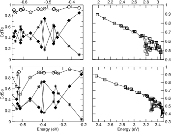
Figure 1: Spectra weight of single particle eigenstates.

In the bulk limit, the conduction band is $S=\frac{1}{2}$ like and the valence band is $J=\frac{3}{2}$ like. We calculate the spectra weight of zero-field single particle eigenstates in terms of local orbitals. In all calculations we adopt an coordinate system in which the z-axis is parallel to the c-axis of the wurtzite structure. We find that for the conduction band, around $90$% of the spectra weight of the band edge state is in $S=\frac{1}{2}$, which increases as the size of nanostructures increases. However for the same nanostructure, the $S=\frac{1}{2}$ component decreases as we move toward higher energy condunction electron states. For the valence band, we find that the band is $J=\frac{3}{2}$ like within a fair large energy window near the valence band edge , containing around 90% of the spectra weight. However the mixing between heavy-hole and light-hole is strong and the mixing is sensative to the size and shape of the nanostructure. It is thus improper to assign the label of heavy-hole or light-hole to the holes states in those nanostructures. In Fig.1 we plot the spectra weight of zero-field eigenstates near the band edges for the 777 atoms CdTe and CdSe nanostructures. Nanostructures containing different number of atoms show qualitatively similar behavior. The main features to be noticed are the reduction of $S=\frac{1}{2}$ ($S=\frac{3}{2}$) components for the electron (hole) states as we move away from the conduction (valence) band edge, and the strong heavy-hole light-hole mixing.

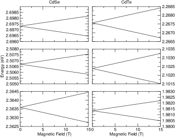
Figure 2: Electron Zeeman splitting for 777 atoms CdSe and CdTe nanostructures.

Figure 3: Hole Zeeman splitting for 777 atoms CdSe and CdTe nanostructures

For zero field energy levels, the band edge states show redshifting as the number of atoms in nanostructures increases. The valence band edge state occurs as heavy-hole like state for some of the nanostructures while occurs as light-hole like state for other nanostructures, even when there is only minor difference in the numbers of atoms contained in nanostructures. This result indicates that the shape of the nanostructure has profound impact on the spin content of the hole states. No degeneracy except for the Kramers’ degeneracy is observed, which we attribute to the strong quantum confinement effect of the small nanostructures. In Fig.2 (Fig.3) we plot the magnetic field dependence of several electron (hole) energy levels for 777 atoms CdSe and CdTe nanostructures. The magnetic field is pointing along the z-direction, which coincides with the c-axis of the wurtzite structure. As seen in these figures, the Zeeman splitting is nearly linear in B. Magnetic field dependence for most of the electron and hole levels calculated in this work show qualitatively the same behavior, while quantitatively the slope of Zeeman splitting varies, giving rise to different g-factors. However some of the electron and hole levels show strongly non-linear dispersions. In Fig. 4 we plot the Zeeman splitting for some of those levels. The non-linear dispersions occur when the intrinsic Zeeman spltting is close to the inter-level spacing, giving rise to level anti-crossing, or when the intrinsic Zeeman splitting is small compared to the splitting induced by inter-doublets couplings.

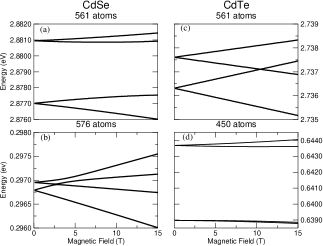
Figure 4: Non-linear Zeeman splittings. (a) Electrons in 561 atoms CdSe nanostructure. (b) Holes in 576 atoms CdSe nanostructure. (c) Electrons in 561 atoms CdTe nanostructure. (d) Holes in 450 atoms CdTe nanostructure.

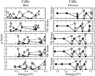
Figure 5: Intrinsic g-factor of first ten electron and hole states for CdSe nanostructures at various sizes. Filled circles represent $g_{z}$ and empty circles represent $g_{x}$.

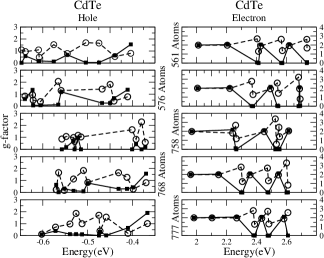
Figure 6: Intrinsic g-factor of first ten electron and hole states for CdTe nanostructures at various sizes. Filled circles represent $g_{z}$ and empty circles represent $g_{x}$.

In Fig.5 (Fig.6) we plot the intrinsic g-factor of first ten electron and hole states for CdSe (CdTe) nanostructures at various sizes. We found that $g_{x}\approx g_{y}\neq g_{z}$ and $g_{y}$ is not plotted for clarity. In Table 1 we summarize the size and aspect ratio of the nanostructures used in Fig.5 and Fig.6. The aspect ratio is defined to be the ratio between $L_{z}$ and the average diameter $\sqrt{L_{x}L_{y}}$ in x-y plane. The prominent features are the redshift (blueshift) of electron (hole) levels and anisotropy of g-factors. Quantitatively we found it difficult to identify a simple scaling relation between the g-factor and size or aspect ratio of nanostructures using the data shown here and other data for smaller size nanostructures. The size ($L_{x},L_{y},L_{z}$) and the aspect ratio are average quantities which are used to characterize the nanostructures. For higher dimensional systems, these average quantities have been successfully used to characterize the g-factors, since the detail of the boundary is less significant. However for small size nanostructures the detail of the structure is important in determining the energy levels, wavefunctions, and hence the g-factors. For example, it is difficult to modify the aspect ratio along without altering substantially the detail shape of the structure. We speculate that this is the main reason to make it difficult to identify a simple scaling relation between g-factor and other averaged quantities. It is thus advantageous to use tight-binding method, which captures the detail of the structure, instead of effective mass approximation type methods.

Qualitatively some observations can be made. First since the g-factor is not a smooth function of the eigenenergy, nearby states might possess very different g-factors. The g-factors also change substantially as the size changes. We observe that some energy levels move toward higher energy while some levels move toward lower energy as one increases the aspect ratio. Similar dependence has been recently observed in the calculation of electronic states of CdSe quantum rods. Hu et al. (2002). We also observe that the electron g-factors are less sensitive than the hole g-factors to the aspect ratio. This can be attributed to the fact that the $S=\frac{1}{2}$ like behavior of the electron is insensitive to the aspect ratio while for the $J=\frac{1}{2}$ like holes, the mixing of heavy-hole and light-hole is sensitive to the aspect ratio.

Table 1: Size and aspect ratio of the nanostructures.

Number of atoms	450	561	758	768	777
$\sqrt{L_{x}L_{y}}$ (Å)	26.76	22.85	34.55	27.42	20.44
$L_{z}$ (Å)	21.88	35.88	35.88	39.38	49.88
Aspect Ratio	0.82	1.64	1.04	1.44	2.44

V Summary and Discussion

In summary we have developed a general method to evaluate electron and hole Zeeman splittings in semiconductor nanostructures within a tight-binding framework. The calculation is carried out within the electron-hole picture instead of the conduction-valence band electron picture. Hence the scheme can be readily extended to the exciton Zeeman splitting calculation by including the electron-hole Coulomb interaction. The results found here are qualitatively similar to the results in Ref Chen and Whaley, 2004, in which only band edge states are calculated. The quantitative difference may be attributed to the approximation used during the transformation to the electron-hole picture. In most cases we observe nearly linear Zeeman splittings induced by the external magnetic field. In some cases we also observe non-linear Zeeman splittings which are due to the interlevel coupling between nearby Kramers’ doublets. Those results are qualitatively similar to what are obtained in Ref Prado et al., 2004.

We find that the behavior of electron Zeeman splittings of nanostructures with different aspect ratio does not show drastic difference. This is in contrast to the drastic difference (change of sign) between spherical quantum dot (SQD) and semi-spherical quantum dot (SSQD) found in Ref Prado et al., 2004. It should be noted that in Ref Prado et al., 2004, SSQD is treated by imposing boundary condition on envelope function, requiring envelope function to be vanishing in the upper hemisphere. This boundary condition is very different from the boundary condition used here for nanostructures with different aspect ratio. In other word, the idea of SSQD in Ref Prado et al., 2004 is different from the idea of quasi-spherical regime for the elongated nanostructure with varying aspect ratio in other references.Schrier and Whaley (2003); Rodina et al. (2003); Chen and Whaley (2004)

There may be strong difference between magneto-optical properties of free electron-hole pairs and excitons, in which the Coulomb interaction is included. Two key questions to be addressed are the effect of the Coulomb interaction and how to experimentally observe electron, hole, and exciton Zeeman splittings using magneto-absorption spectroscopy. To answer the first question one has to estimate how strongly the electron-hole Coulomb interaction modifies the free electron-hole pair picture. In Ref Leung et al., 1998, a restricted basis, single excitation configuration interaction representation method is used to calculate the exciton fine structure for CdSe nanostructures. It was shown that about 18 electron and 24 hole single-particle states needed to be included to get a reasonable accurate exciton energy. We expect that roughly the same number of states will be needed in order to accurately evaluate the exciton Zeeman splittings. Since our results indicate that the g-factor of electrons and holes may vary substantially from one state to another, we expect that the exciton g-factor may be very different from the simple sum of the g-factor of free electrons and holes. Starting from the general framework developed here, the effect of Coulomb interaction can be included via configuration interaction methodLeung and Whaley (1997); Leung et al. (1998) or time-dependent tight-binding method.Hill and Whaley (1996)

To shed some light on the second question we have to consider the problem of optical orientation in nanostructures. In bulk or quantum well materials, one typically assumes that the conduction band edge is s-like while the valence band edge is heavy-hole like. In this case the optically active excitons only consist of heavy-holes. Due to the angular momentum conservation, the optically excited electron and heavy-hole spin will be aligned in particular configuration depending on the polarization of the optical pulse. However, in nanostructures the strong heavy-hole light-hole mixing and the Coulomb interaction break down this naive picture, as it becomes difficult to determine the spin configuration of the constituent electrons and holes of the excitons. A realistic calculation of the optical absorption oscillator strength might be needed in order to fully understand what is actually measured in the experiment.