Quasi-stationary evolution of systems driven by particle evaporation

Abstract

We study the quasi-stationary evolution of systems where an energetic confinement is unable to completely retain their constituents. It is performed an extensive numerical study of a gas whose dynamics is driven by binary encounters and its particles are able to escape from the container when their kinetic energies overcome a given cutoff $u_{c}$. We use a parametric family of differential cross sections in order to modify the effectiveness of this equilibration mechanism. It is verified that when the binary encounters favor an effective exploration of all accessible velocities, the quasi-stationary evolution is reached when the detailed balance is imposed for all those binary collisions which do not provoke particle evaporation. However, the weakening of this effectiveness leads to energy distribution functions which could be very well fitted by using a Michie-King-like profile. We perform a theoretical analysis, in the context of Hamiltonian systems driven by a strong chaotic dynamics and particle evaporation, in order to take into account the effect of the nonhomogeneous character of the confining potential.

I Introduction

Gravitation is a generic example of a selfgravitating interaction which is not able to effectively confine particles: it is always possible that some of them reach the sufficient energy for escaping from a putative system, so that the astrophysical systems undergo an evaporation process, and therefore, they will never be in a real thermodynamic equilibrium. This is precisely the origin of the long-range singularity of the thermodynamical description of astrophysical systems antonov ; Lynden ; ruelle ; lind ; thirring ; kies ; pad ; gross ; de vega ; chava .

On the other hand, the N-body gravitating systems satisfy a strong chaos criterion (see Ref.pet ), supporting the assumption of an increasingly uniform spreading of orbits over the constant energy surface or its intersection with any other integral of motion as the angular momentum. The competition of these dynamical behaviors produces the achievement of a quasi-stationary regime in the evolution of the astrophysical systems, allowing in this way the applicability of some ordinary equilibrium statistical mechanics methods antonov ; Lynden ; ruelle ; lind ; thirring ; kies ; pad ; gross ; de vega ; chava ; pet .

The aim of the present paper is to study the quasi-stationary evolution of systems driven by a conservative microscopic dynamics which is also strongly affected by particle evaporation. Our focus will be mainly on the analysis of the effect of evaporation under the modification of the efficiency of the equilibration mechanisms (sections II and III ). The interest in such study is justified as follows.

As discussed elsewhere, the equilibration mechanisms are closely connected with the chaotic properties of the microscopic dynamics. This last ones explain both, qualitatively and quantitatively, whether or not the dynamics provides an effective exploration of all those accessible microscopic configurations, and consequently, of how strong is the system tendency towards its equilibration pet ; arnold ; sinai ; fermi ; cohen ; krylov . Hence, it is clearly evident that the influence of a dissipative process, as the particle evaporation, is significantly affected by how efficient are the system’s equilibration mechanisms.

On the other hand, as a by-product of the above study, we will perform in section IV a theoretical analysis of the effect of evaporation on the distribution function over the single particle six-dimensional $\mu$-phase space, $f\left(\mathbf{r},\mathbf{p}\right)$. This analysis is carried out in the context of Hamiltonian systems driven by a very strong chaotic dynamics, and our interest is the consideration of the nonhomogeneous character of the confining interaction. The result is contrasted with the requirements of the Jeans theorem jeans for the collisionless selfgravitating systems, as well as to the Michie-King model of globular clusters and elliptical galaxies king ; spitzer ; chandra ; bin .

II A simple model

It was done in the past an important set of works devoted to the analysis of particle evaporation in the context of astrophysical systems in the framework of binary encounters (see for example in king ; spitzer ; chandra ; bin and references therein). We are interested in performing a numerical closer look at of these studies by considering the binary collisions from a perspective which allows us to control the effectiveness of this equilibration mechanism.

Considering the general lines of the classical paper of Spitzer and Härm spitzer , we assume that the following idealizations procee: The potential energy is constant within the volume of the system with spherical symmetry, but vanishes in the outside region:

$$u\left(r\right)=\left\{\begin{array}[c]{cc}-u_{c}&r\leq R\\ 0&r>R\end{array}\right..$$ (1)

This first idealization disregards the effects of the nonhomogeneous character of the confining interaction, and therefore, this self-gravitating model is equivalent to a gas of particles enclosed in a special container which allows a given particle to escape when its kinetic energy overcomes a given cutoff $u_{c}$. The second idealization is to assume that the particle mean-free-path is many times the characteristic size (or length scale) of the system, which allows us to take into account only binary collisions. Consequently, a given particle that gains sufficient velocity after a collision will evaporate, since the probability that this particle loses the excessive energy before escaping from container is very small. The third idealization is to suppose that the system is embedded in a bidimensional space.

The following toy dynamics will be taken into account in order to perform a numerical study of the above model. Let us consider a system with $N$ particles and assign to each of them a vector velocity $\mathbf{v}$ and a binary number $b$, being $\mathbf{v}_{k}$ and $b_{k}$ the corresponding data for the k-th particle. The binary number $b=0$ indicates that the corresponding particle has escaped from the system, or to the contrary, that it remains trapped when $b=1$. The dynamical evolution of the model system is carried out as follows:

• For each computational step, a sample of $M$ interacting pairs are chosen one by one at random.

• The pair interaction is suppressed when at least one particle has already escaped from the system.

• When the pair interaction is possible, the particles change their velocities as follows:

  $$\mathbf{\tilde{v}}_{1,2}=\frac{\mathbf{v}_{1}+\mathbf{v}_{2}}{2}\pm\left|\frac{\mathbf{v}_{1}-\mathbf{v}_{2}}{2}\right|\mathbf{n},$$ (2)

  being $\mathbf{n}$ an unitary vector defined by:

  $$\mathbf{n}=\left[\cos\left(\theta_{0}+\theta\right),\sin\left(\theta_{0}+\theta\right)\right],$$ (3)

  where the phase $\theta$ takes a random value belonging to the interval $\left(-\pi,\pi\right)$, being $\theta_{0}$ the phase of the relative velocity $\mathbf{v}=\left(\mathbf{v}_{1}-\mathbf{v}_{2}\right)/2$. The above equation ensures the energy and linear momentum conservation of the pair during the collision. If after the collision the kinetic energy of a given particle of the pair is greater than the escape energy $u_{c}$, its corresponding binary number changes to zero, which means that this particle has escaped from the system.

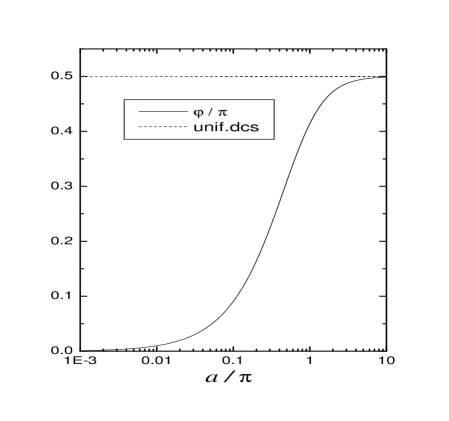
• The random phase $\theta$ is distributed according to the following generic differential cross section:

  $$d\sigma\left(\theta;a\right)=\frac{\sigma}{2K}\frac{ad\theta}{a^{2}+\theta^{2}},$$ (4)

  where $\sigma$ is the total cross section, $a$, a positive real parameter which drives the form of the interaction, and $K$, a normalization constant, $K=\arctan\left(\pi/a\right)$.

The specific form of the differential cross section (4) allows us to carry out a comparative study of the quasi-stationary evolution features when the efficiency of the equilibration mechanism is modified: the variation of the deformation parameter $a$ affects the way that the binary encounters allow the particles to explore the velocities which are stable under the evaporation.

The FIG.1 shows the effect of the deformation parameter $a$ on the angle $\varphi$ in which is enclosed the $50$ % of the binary encounters, $\left|\theta\right|\leq\varphi$. When $a$ is large enough, the expression (4) becomes in a uniform distribution:

$$d\sigma\left(\theta\right)\simeq\sigma\frac{d\theta}{2\pi},$$ (5)

which will be used as a reference.

Figure 1: Effect of the deformation parameter $a$ in the angle $\varphi$ in which is enclosed the $50$ % of deflections during the binary encounters, that is, $\varphi=a\tan\left[0.5\arctan\left(\frac{\pi}{a}\right)\right]$. Dash line represents the asymptotic value for the uniform differential cross section (5).

Let $N_{1}$ be the number of particles remaining in the system. We consider the $\rho=N_{1}/N$ as the relative density of the gas. We denoted by $\epsilon$, the kinetic energy per particle of all those particles remaining in the system, that is:

$$\epsilon=\frac{1}{N_{1}}\sum_{k=1}^{N}b_{k}\frac{1}{2}\mathbf{v}_{k}^{2}\;\text{.}$$ (6)

The probability that the interaction takes place for a given pair is:

$$p_{\text{coll}}=\frac{N_{1}\left(N_{1}-1\right)}{N\left(N-1\right)}\simeq\rho^{2},$$ (7)

being $N_{1}$ and $N$ large enough. The expectation value of collisions which take place in a computational step, $c$, can be estimated by $c\simeq Mp_{\text{coll}}\simeq M\rho^{2}$.

According to the kinetic theory of gases, the rate of collision events per the time unit, $\omega$, can be estimated as $\omega\simeq\frac{1}{2}\sigma n^{2}\bar{v}V$, being $\sigma$ the total cross section of the particles, $n$, the particles per unit of volume, $\bar{v}$, the expectation value of the relative velocity among the particles of the system, while $V$ is the volume of the gas container. Let $\Delta t$ be the temporal increment in each computational step. Since $c\sim\omega\Delta t$, a direct comparison allows us to set the equivalences: $\rho\sim n$, $N\sim V$, and therefore, the number of samples is each computational step should grow proportional to the system size, that is, $M\simeq\mu N$, where $\mu\equiv\frac{1}{2}\sigma n_{0}\bar{v}\Delta t$, being $n_{0}$ the initial density of particles per unit of volume. If $m$ represents the particles mass, the characteristics units for velocity and time are the following: $v_{c}=\sqrt{2u_{c}/m},~{}\tau_{0}=2/\sigma n_{0}v_{c},$where $v_{c}$ is also the cutoff velocity. The temporal increment in each computational step $\Delta t$ can be estimated by using the average relative velocity among the particles of the system as $\Delta t=\lambda_{0}\mu/\bar{v}$, being:

$$\bar{v}=\frac{2}{N_{1}\left(N_{1}-1\right)}\sum_{k=1}^{N-1}\sum_{j=k+1}^{N}b_{k}b_{j}\left|\mathbf{v}_{k}-\mathbf{v}_{j}\right|,$$ (8)

and $\lambda_{0}=v_{c}\tau_{0}$, the characteristics particle mean-free-path.

II.1 Thermodynamical limit

It could be spoken about a continuous distribution of the particles velocities when $N$ tends to infinity because of the particles fill densely all the accessible velocities. Let $n\left(\mathbf{v},\tau\right)d^{2}\mathbf{v}$ be the relative density of those particles remaining in the system whose velocities are located inside the differential region $\left(\mathbf{v},\mathbf{v}+d\mathbf{v}\right)$ in a given computational step $\tau$. The function $n\left(\mathbf{v},\tau\right)$ represents the relative density distribution function of particles in the neighborhood of the point $\mathbf{v}$ in the space of admissible velocities $\Sigma\equiv\left\{\mathbf{v}\in\mathbf{R}^{2}:\mathbf{v}^{2}<v_{c}^{2}\right\}$. The variation of $n\left(\mathbf{v},\tau\right)$ in the next computational step $\tau+\delta\tau$ can be expressed as follows:

$$\frac{\delta}{\delta\tau}n\left(\mathbf{v},\tau\right)=\mu\left[I_{in}\left(\mathbf{v};\tau\right)-I_{out}\left(\mathbf{v};\tau\right)\right],$$ (9)

being $I_{in}\left(\mathbf{v};\tau\right)$ the probability of some particles to reach a final velocity $\mathbf{v}$ after a collision, while $I_{out}\left(\mathbf{v};\tau\right)$ represents the probability of some particles with initial velocity $\mathbf{v}$ to experience a collision in the next computational step. These probabilities are given by the formulae:

$$I_{in}\left(\mathbf{v};\tau\right)={\displaystyle\iint\limits_{\Sigma\times\Sigma}}d^{2}\mathbf{v}_{1}d^{2}\mathbf{v}_{2}~{}K\left(\left.\mathbf{v}\right|~{}\mathbf{v}_{1},\mathbf{v}_{2}\right)n\left(\mathbf{v}_{1},\tau\right)n\left(\mathbf{v}_{2},\tau\right),$$ (10)

$$I_{out}\left(\mathbf{v};\tau\right)=n\left(\mathbf{v},\tau\right)\underset{\Sigma}{\int}d^{2}\mathbf{v}_{1}n\left(\mathbf{v}_{1},\tau\right),$$ (11)

being $K\left(\left.\mathbf{v}\right|~{}\mathbf{v}_{1},\mathbf{v}_{2}\right)$ the probability that a given particle of the collision pair with initial velocities $\left(\mathbf{v}_{1},\mathbf{v}_{2}\right)$ to reach $\mathbf{v}$ as a final velocity:

$$K\left(\left.\mathbf{v}\right|\mathbf{~{}v}_{1},\mathbf{v}_{2}\right)=\int_{0}^{2\pi}~{}\frac{d\sigma\left(\theta\right)}{\sigma}\delta\left[\mathbf{v-v}\left(\mathbf{v}_{1},\mathbf{v}_{2};\theta\right)\right],$$ (12)

being

$$\mathbf{v}\left(\mathbf{v}_{1},\mathbf{v}_{2};\theta\right)=\frac{\mathbf{v}_{1}+\mathbf{v}_{2}}{2}+\left|\frac{\mathbf{v}_{1}-\mathbf{v}_{2}}{2}\right|\mathbf{n}\left(\theta_{0}+\theta\right),$$ (13)

and $d\sigma\left(\theta\right)$ the differential cross section for the binary encounters. The difference between $I_{in}$ and $I_{out}$ extracts out all those cases in which the interacting particles keep the same velocities after the interaction.

Figure 2: Geometrical visualization of the inequality (15).

The specific form of the irreversible dynamical equation (9) leads to some straightforward consequences. Because the probability $p\left(\mathbf{v}_{1},\mathbf{v}_{2}\right)$ that a given particle of the collision pair $\left(\mathbf{v}_{1},\mathbf{v}_{2}\right)$ to remain in the system after the collision:

$$p\left(\mathbf{v}_{1},\mathbf{v}_{2}\right)=\underset{\Sigma}{\int}d^{2}\mathbf{v~{}}K\left(\left.\mathbf{v}\right|~{}\mathbf{v}_{1},\mathbf{v}_{2}\right),$$ (14)

may differ from the unity, $0\leq p\left(\mathbf{v}_{1},\mathbf{v}_{2}\right)\leq 1,$ the total relative density of the system $\rho\left(\tau\right)=\int_{\Sigma}d^{2}\mathbf{v~{}}n\left(\mathbf{v},\tau\right)$ will decrease or remain constant:

$$\frac{\delta}{\delta\tau}\rho\left(\tau\right)=-\mu{\displaystyle\iint\limits_{\Sigma\times\Sigma}}d^{2}\mathbf{v}_{1}d^{2}\mathbf{v}_{2}~{}q\left(\mathbf{v}_{1},\mathbf{v}_{2}\right)n\left(\mathbf{v}_{1},\tau\right)n\left(\mathbf{v}_{2},\tau\right)\leq 0,$$ (15)

being $q\left(\mathbf{v}_{1},\mathbf{v}_{2}\right)=1-p\left(\mathbf{v}_{1},\mathbf{v}_{2}\right)$, the escaping probability.

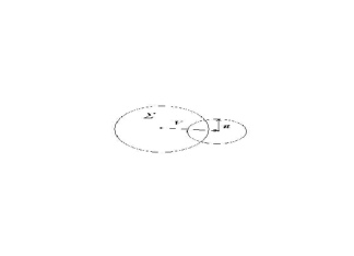
A geometrical visualization of the inequality (15) is shown in FIG.2. Here $\mathbf{\Sigma}$ is the admissible subset of velocities in $\mathbf{R}^{2}$; $\mathbf{V}$ represents the velocity of the center of mass, $\mathbf{V}=\frac{1}{2}\left(\mathbf{v}_{1}+\mathbf{v}_{2}\right)$, while $\mathbf{u}$ is the final velocity of the specific particle in the center of mass frame, that is, $\mathbf{u}=\frac{1}{2}\left|\mathbf{v}_{1}-\mathbf{v}_{2}\right|\mathbf{n}\left(\theta_{0}+\theta\right)$. Only those values of the vector addition $\mathbf{v}=\mathbf{V+u}$ belonging to $\mathbf{\Sigma}$ correspond to the final state where the specific particle of the pair remains in the system after the collision. In the particular case of the uniform differential cross section (5), $p\left(\mathbf{v}_{1},\mathbf{v}_{2}\right)$ is numerically equal to fraction of the circumference perimeter described by the vector $\mathbf{u}$ belonging to the subset $\mathbf{\Sigma}$. A simple geometrical analysis yields the following expression for this probability:

$$p\left(\mathbf{v}_{1},\mathbf{v}_{2}\right)=\left\{\begin{array}[c]{cc}0&\text{when }x\leq-1\\ \frac{1}{2}+\frac{1}{\pi}\arcsin\left(x\right)&\text{when }\left|x\right|<1\\ 1&\text{when }x\geq 1\end{array}\right\},$$ (16)

where $x$ is given by:

$$x=\frac{v_{c}^{2}-\mathbf{V}^{2}-\mathbf{u}^{2}}{2\left|\mathbf{V}\right|\left|\mathbf{u}\right|}\;\text{.}$$ (17)

It is evident that only those collision pairs satisfying the condition:

$$\frac{1}{2}\left|\mathbf{v}_{1}+\mathbf{v}_{2}\right|+\frac{1}{2}\left|\mathbf{v}_{1}-\mathbf{v}_{2}\right|\leq v_{c},$$ (18)

will remain in the system after the interaction with a $100$ % of probability, and this condition does not depend on the differential cross section used to describe the binary collisions, nor on the dimension of the space.

As already shown, the relative density distribution function $n\left(\mathbf{v};\tau\right)$ obeys a nonlinear irreversible dynamics, which is also dissipative. Thus, the evaporation is explicitly taken into account in the dynamical equation of the system. The nonlinear nature of equation (9) is a feature making the difference from the standard treatment of evaporation by using a linear Fokker-Planck equation applied to the astrophysical systems bin ; chandra ; spitzer ; king . This equation does not necessarily lead to exponential decays of the particles number with the time.

II.2 Numerical experiments

We set without lost of generality $m=1$, $\lambda_{0}=1$ and $u_{c}=2.6$ in our numerical study of dynamics. The number $M$ of interacting pair chosen in a given computational step was settled to be $M=\left[\mu N\right]$, where $\mu=0.05$, in order to ensure a smooth temporal evolution of the physical observables. We start from an initial configuration where all particles belong to the system, that is, $b_{k}=1$, $\forall k\in\left[1,2,...N\right]$. Preliminary runs by using the uniform differential cross section (5) allows us to set $N=1000$, since size effects are not significant when we compare the results obtained by considering $N=500$ and $1000$.

We are interested in describing some kind of dynamical evolution of the model system which could be considered as a quasi-stationary regime. To this aim we take into account the following initial distribution functions of particle energies:

• Uniform Distribution (UNIC):

  $$\omega_{I}\left(e\right)=\frac{1}{E_{1}}\times\left\{\begin{array}[c]{cc}1&\text{with }0\leq e<E_{1}<u_{c}\\ 0&\text{otherwise}\end{array}\right.,$$ (19)

• Truncating Boltzmann Distribution (TBIC):

  $$\omega_{II}\left(e\right)=\frac{\beta\exp\left(-\beta e\right)}{1-\exp\left(-\beta u_{c}\right)}\times\left\{\begin{array}[c]{cc}1&\text{ with }0\leq e<u_{c}\\ 0&\text{otherwise}\end{array}\right.,$$ (20)

• Double Size Uniform Distribution (DSIC):

$$\omega_{III}\left(e\right)=\frac{1}{E_{2}-E_{1}}\times\left\{\begin{array}[c]{cc}1&\text{with }E_{1}<e<E_{2}<u_{c}\\ 0&\text{otherwise}\end{array}\right.,$$ (21)

where $E_{1}$, $E_{2}$ and $\beta$ are positive real parameters. The particles velocities were uniformly distributed at random in all possible directions $\left(0,2\pi\right)$ for the three initial conditions.

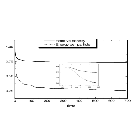
We start from an initial condition UNIC with $E_{1}=2.0$ by using the uniform differential cross section. FIG.3 shows the dynamical evolution of $\rho$ and $\epsilon$ in terms of the physical time $t$. It is easily seen that the system experiences a sudden relaxation process in which the $25$ % of the particles is evaporated in the first stages of the evolution. There, the system enters in a long transient regime where the evaporation events have been extremely reduced, but they still take place causing a slow variation of the kinetic energy per particle.

The insert graph evidences that this relaxation process is progressive, that is, no real equilibrium configuration seems to be reached by extending the computational simulation of the dynamics, but the rate of the evolution seems to be continuously reduced.

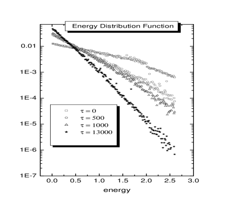
Let us analyze now the effect of the particle evaporation in the energy distribution function of the system. We will apply the following procedure in order to obtain an appreciable statistics of the microscopic configurations around a given computational step $\tau$:  We carry out certain number $v$ of virtual trajectories, with $100$ computational steps each, by starting from the initial configuration at the computational step $\tau$. The data is collected by considering $20$ microscopic configurations in each of such virtual trajectories, and therefore, a total of $20v$ microscopic configurations are taken into account in order to build the energy distribution function. This procedure is applied in the successive analysis.

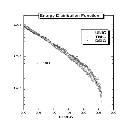
FIG.4 shows the energy distribution function by considering $100$ virtual trajectories: at the first stages of the evolution with $\tau=0,500,1000$, and a final configuration when $\tau=13000$. It is remarkable that after a very short relaxation, the energy distribution function is stabilized in a truncating Boltzmann distribution of the form given in the equation (20), which is easily evidenced in the linear dependence of the distribution functions shown in this figure by using a logarithmic scale. The existence of this profile allows us to claim that the system exhibits a quasi-stationary evolution where the relative density $\rho$ and the energy per particle $\epsilon$ seem to be the macroscopic control variables along the successive dynamics of the system.

Figure 3: Dynamical evolution of the relative density $\rho$ and the kinetic energy per particle $\epsilon$ by using the uniform differential cross section with UNIC initial condition with $E_{1}=2.0$. The same dependences are shown in the insert graph by using a logarithmic scale for the time variable.

Figure 4: Energy distribution function along the dynamical evolution shown in FIG.3. The system seems to stabilize in a Truncating Boltzmann distribution.

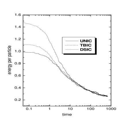
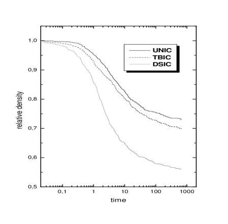
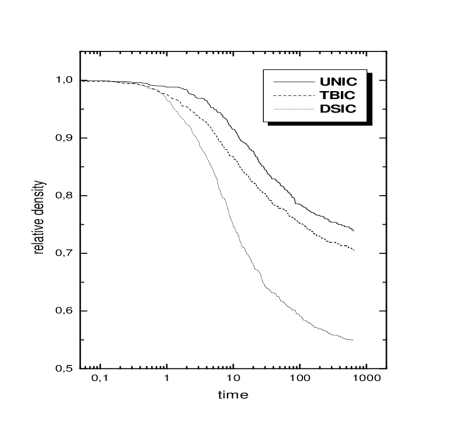
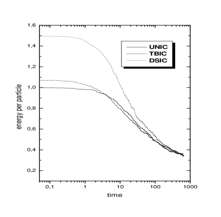
Let us now perform a comparative study in order to clarify the possible influence of the initial conditions in the nature of the quasi-stationary evolution of the system. We consider three initial conditions for this analysis: $a$) UNIC: $E_{1}=2.0$; $b$) TBIC: $\beta=0.25$; $c$) DSIC: $E_{1}=1.0$ and $E_{2}=2.0$. The results are shown in FIG.5 and FIG.6. As expected, the particle evaporation depends strongly on the initial microscopic configurations. However, the energy per particle $\epsilon$ quickly tends to a regime where the successive evolution is so slow that the dynamical evolutions of this observable starting from different initial microscopic configurations converge asymptotically all them.

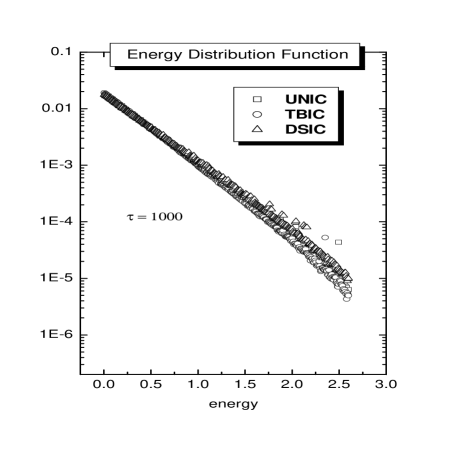
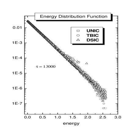
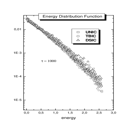
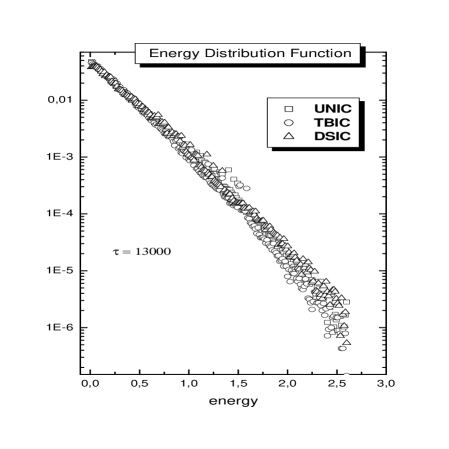
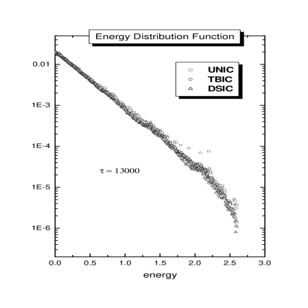
FIG.7 and FIG.8 show the energy distribution functions for these initial conditions at two different computational times by considering also $100$ virtual trajectories: FIG.7 at $\tau=1000$, and FIG.8 at $\tau=13000$. These results strongly suggest us that the Truncating Boltzmann distribution (20) is the quasi-stationary profile appearing in the dynamical evolution of a gas of particles driven by binary encounters which undergoes particle evaporation by using the uniform differential cross section. The great similarity among these profiles is a consequence of the sudden evolution of the system towards configurations whose energy per particle is around $\epsilon\simeq 0.27$. For this energy the evaporation rate is so low that the subsequent dynamics spends too much time for exhibiting a significant variation.

All those interacting particles whose kinetic energies are less than $u_{c}/2$ do not provoke evaporation events, and therefore evaporation events could be only produced when a particle, whose energy $e$ belongs to the energetic range $\frac{1}{2}u_{c}\leq e\leq u_{c}$, is involved in a binary encounter. This is precisely the origin of the slow dynamical evolution observed in the above numerical experiment when $\epsilon\simeq 0.27$: Most of the particles remaining in the system belong to the stable region $0\leq e\leq\frac{1}{2}u_{c}$.

Figure 5: Dynamical evolution of the relative density by using three different initial conditions and the uniform differential cross section.

Figure 6: Dynamical evolution of the energy per particle by using three different initial conditions and the uniform differential cross section.

Figure 7: Energy distribution function at $\tau=1000$ for the dynamical evolution shown in FIG.5 and FIG.6.

Figure 8: The same observable shown in FIG.7, but this time at $\tau=13000$.

Figure 9: Dynamical evolution of the relative density $\rho$ when a moderate asymmetry among large and short deflections is considered.

Figure 10: Dynamical evolution of the energy per particle $\epsilon$ by using a moderate asymmetry among large and short deflections.

Figure 11: Energy distribution function at $\tau=1000$ for the dynamical evolutions shown in FIG.9 and FIG.10.

Figure 12: The same observable shown in FIG.11, but this time at $\tau=13000$.

As already noted, the uniform differential cross section (5) allows a given interacting pair to explore; in an effective fashion, all those possible results of their collision event, and therefore, large variations of the kinetic energies of the interacting particles are very likely. We are interested in analyzing if the quasi-stationary profile obtained above remains unchanged even when the collision events are not so effective, that is, when large variations of the kinetic energy of the collision particles are not so favored. This analysis can be performed by using the differential cross section (4) with $a=0.2\pi$. As already shown in FIG.1, this particular value produces a moderate asymmetry among large and short deflections angles during the binary encounters, and therefore, a weaker effectiveness of the equilibration mechanism with regard to the uniform case.

Figure 13: Dynamical evolution of the relative density $\rho$ by using a differential cross section with a great asymmetry between short and large deflections.

Figure 14: Dynamical evolution of the energy per particle $\epsilon$ by using a differential cross section with a great asymmetry between short and large deflections.

Figure 15: Energy distribution function at $\tau=1000$ for the dynamical evolutions shown in FIG.13 and FIG.14.

Figure 16: The same observable shown in FIG.15, but this time at $\tau=13000$.

We implement the same initial conditions used in the previous study. The dynamical evolution of the relative density $\rho$ and the energy per particle $\epsilon$ are shown in FIG.9 and FIG.10, respectively. Despite we have considered a new microscopic interacting picture for the binary encounters, it is evident here that no significant qualitative differences are exhibited in the dynamical behavior of these observables. This conclusion is reinforced by looking at the results showed in FIG.11 and FIG.12, where it can be appreciated the persistence of the truncating Boltzmann profile (20) even after using a moderate asymmetry among large and short deflections, although there is a slight tendency to a reduction of the particles population for the large energies with a significant incidence of fluctuations.

Let us now consider a very asymmetric differential cross section. We repeat the same numerical experiment described above, but this time by considering $a=0.02\pi$. This value of the deformation parameter $a$ leads to a predominance of the small variation of the kinetic energies of the collision particles, and therefore, a significant reduction of the effectiveness of the microscopic dynamics in reaching their quasi-equilibrium conditions.

The evolution of $\rho$ and $\epsilon$ are shown in FIG.13 and FIG.14. In a similar way, the energy distribution functions when $\tau=1000$ and $13000$, in FIG.15 and FIG.16 is also shown after running 200 virtual trajectories. As expected, the rate of evaporation has been reduced. The energy distribution function clearly evidences a new qualitative effect of the evaporation, which is more accentuated in FIG.15. The results shown in these figures evidence a significant deviation of the distribution function from the linear dependence close of the energy cutoff $u_{c}$, without vanishing at this energy.

Let us now investigate, qualitatively, these quasi-stationary profiles by using a Michie-King-like distribution bin :

$$\omega_{M-K}\left(e\right)=C_{0}\langle\exp\left[-\beta e\right]-\exp\left(-\beta\varepsilon_{C}\right)\rangle,$$ (22)

with $0\leq e\leq u_{c}$, being $u_{c}\leq\varepsilon_{C}<+\infty$. It is easy to note that when $\varepsilon_{C}$ decreases from the infinity towards the cutoff energy $u_{c}$, the energy parameter $\varepsilon_{C}$ causes a continuous deformation of the Truncating Boltzmann profile (20) towards the well-known Michie-King profile of the globular clusters bin ; king .

Figure 17: Energy Distribution function with $a=0.02\pi$ at different energy per particles with their fitting by using the Michie-King like profile. The insert plot shows the energy dependence of the parameter $\varepsilon_{C}$.

Figure 18: Energy Distribution Function when $\epsilon=1.0$ for different values of deformation parameter $a$. The insert plot shows the dependence $\varepsilon_{C}$ versus $a$.

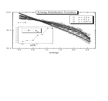
We perform several runs and obtain the energy distribution functions at different energies, starting from a TBIC initial condition with $\beta=0.01$. These results are shown in FIG.17. The reader can notice that the profile (22) offers a fairly good fitting for all these dependences, although for the case where $\epsilon=0.4$ some discrepancies are evident. Such differences probably originate from the method used to obtain the distribution functions. The insert plot suggests a weak dependence of the parameter $\varepsilon_{C}\,$ on the energy per particle $\epsilon$.

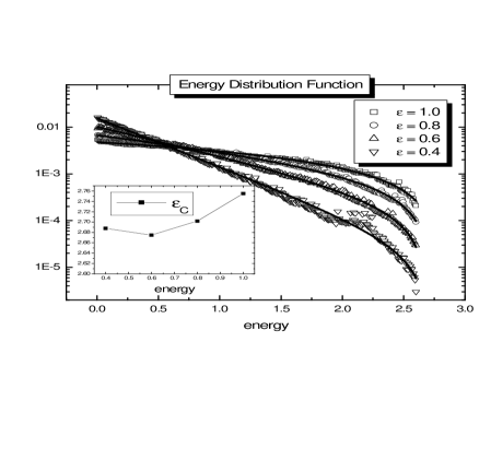
We repeat the calculations by considering different values of the deformation parameter $a$ and keeping the energy per particle fixed at $\epsilon=1.0$. These results are shown in FIG.18. It is clearly evidenced how the energy population at large energies is increased when $a$ decreases, which could be quantitatively described by the decreasing of the parameter $\varepsilon_{C}$. The origin of this behavior follows from the fact that the evaporation events take place practically when the involved particles are those of kinetic energy close to the scape energy $u_{c}$. As already noted, the effect of the correction to the exponential profile is more noticeable with the increasing of the energy per particle $\epsilon$. Apparently, the specific values of $\epsilon$ for the profiles shown in FIG.11 and FIG.12 do not allow us to observe this effect, which is more evident for the results shown in FIG.18.

Summarizing:  The above numerical experiments allow us to conclude that the gas driven by conservative binary encounters and particle evaporation follows certain quasi-stationary evolution which seems to be macroscopically controlled by the energy per particle and the particles density. The generic form of the quasi-stationary profiles is practically independent of the initial conditions, being appropriately describe by a Boltzmann profile truncated at the escape energy when the binary encounters favor an effective exploration of all velocities stable under the evaporation. The reduction of the effectiveness of this equilibration mechanism produces a continuous deformation of the truncating Boltzmann profile towards the well-known Michie-King distribution bin ; king , which could be qualitatively described by the profile shown by equation (22).

III Generic treatment

Let us consider the evaporation of the gas of binary encounters in a more general framework. Let $P_{m}$ be the probability that a given particle be in the state $m$, where $m$ represents certain admissible velocity. The rate of change of this probability, $\mathcal{K}_{m}\left(P\right)$:

$$\frac{dP_{m}}{d\tau}=\mathcal{K}_{m}\left(P\right),$$ (23)

can be divided in two terms as follows:

$$\mathcal{K}_{m}\left(P\right)=\left\langle\text{Eq.Trans}\right\rangle_{m}+\left\langle\text{NEq.Trans}\right\rangle_{m}.$$ (24)

The term $\left\langle\text{Eq.Trans}\right\rangle_{m}$ considers all those binary encounters affecting the state $m$ without provoking evaporation events:

$$\left\langle\text{Eq.Trans}\right\rangle_{m}=\sum_{AB\tilde{m}}W_{\left(AB\right)\left(m\tilde{m}\right)}\left(P_{A}P_{B}-P_{m}P_{\tilde{m}}\right),$$ (25)

while $\left\langle\text{Evap.Trans}\right\rangle_{m}$ involves all those encounters where a collision particle escapes from the system:

$$\left\langle\text{Evap.Trans}\right\rangle_{m}=\sum_{ij}D_{\left(ij\right)m}P_{i}P_{j}-\sum_{st}D_{\left(sm\right)t}P_{s}P_{m}.$$ (26)

It is very easy to note that the transition probability $W_{\left(AB\right)\left(m\tilde{m}\right)}$ of the first term involves four admissible states, while the transition probability $D_{\left(ij\right)m}$ of second one only involves three states. This is the origin of the particles and energy dissipation by evaporation events, which are described by the equations:

$$\frac{dP}{d\tau}=\mathcal{K}\left(P\right),~{}\frac{dE}{d\tau}=\mathcal{R}\left(P\right)$$ (27)

being $P=\sum_{m}P_{m}$ and $E=\sum_{m}\varepsilon_{m}P_{m}$, where $\varepsilon_{m}$ represents the energy of the particle at the m-th state, as well as:

$$\mathcal{K}\left(P\right)=-\sum_{ijm}D_{\left(ij\right)m}P_{i}P_{j},$$ (28)

and

$$\mathcal{R}\left(P\right)=-\sum_{ijm}D_{\left(ij\right)m}P_{i}P_{j}\left(\varepsilon_{i}+\varepsilon_{j}-\varepsilon_{m}\right).$$ (29)

Let us now introduce the normalized distribution function $f_{m}=P_{m}/P$ ( $\sum_{m}f_{m}=1$ ), which obeys the dynamical equations:

$$\frac{df_{m}}{d\tau}=P\left[\mathcal{K}_{m}\left(f\right)-f_{m}\mathcal{K}\left(f\right)\right],$$ (30)

where $\mathcal{K}_{m}\left(f\right)$ and $\mathcal{K}\left(f\right)$ were defined at the equations (24) and (28).

Two important macroscopic quantities of this system are the energy per particle $\epsilon\left[f\right]$ and the entropy functional $s\left[f\right]$:

$$\epsilon\left[f\right]=\sum_{m}\varepsilon_{m}f_{m},~{}s\left[f\right]=-\sum_{m}f_{m}\ln f_{m}.$$ (31)

Since the distribution function $f_{m}$ must be macroscopically controlled by the energy per particle $\epsilon$ during the quasi-stationary regime, the entropy $s\left[f\right]$ versus $\epsilon$ plane must exhibits certain sequence revealing a functional dependence among these macroscopic quantities. FIG.19 confirms this supposition by using three different initial conditions and considering $a=0.02\pi$ in the differential cross section (4).

Figure 19: The plane $s$ versus $\epsilon$ reveals us that the model system follows certain sequence A-B along its dynamical evolution which does not depend on the initial conditions, being this a clear manifestation of its quasi-stationary character. The curve A’-B’ is the quasi-stationary sequence when $a=10.0\pi$. The thick arrow represents the direction of the dynamical evolution along these sequences.

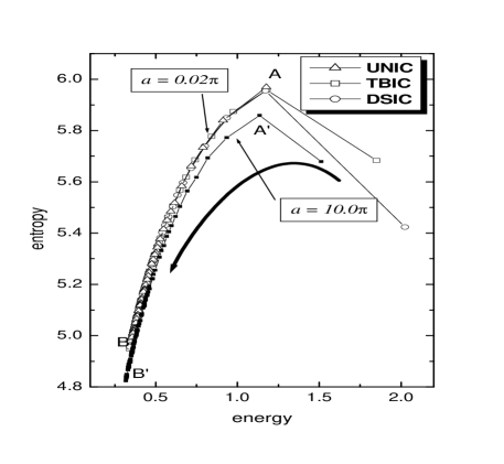
The reader can notice that after a fast relaxation the entropy $s$ evolves along certain curve A-B in the plane $s$ versus $\epsilon$ which does not depend on the initial conditions. This is a clear manifestation of the quasi-stationary character of the dynamical evolution of the model system. Despite the reduction of the effectiveness of the equilibration mechanisms for low values of the deformation parameter $a$, the quasi-stationary character of the dynamical evolution of the model system seems to very robust. For comparison, we also show in this figure the quasi-stationary sequence when $a=10.0\pi$. It is easy to see that the decreasing of the deformation parameter $a$ provokes an increasing of disorder for a given energy per particle, which is directly related with the increasing of the particles population at large energies (see FIG.18).

The energy per particle $\epsilon\left[f\right]$ evolves according to the equation:

$$\frac{d}{d\tau}\epsilon\left[f\right]=P\left\{-\mathcal{K}\left[f\right]\epsilon\left[f\right]+\mathcal{R}\left[f\right]\right\},$$ (32)

being $\mathcal{R}\left[f\right]$ the functional of the equation (29), while the dynamics of the entropy functional $s\left[f\right]$ is described by the equation:

$$\frac{d}{d\tau}s\left[f\right]=P\left\{-\mathcal{K}\left[f\right]s\left[f\right]+\mathcal{W}\left[f\right]+\mathcal{D}\left[f\right]\right\},$$ (33)

where $\mathcal{W}\left[f\right]$ is given by:

$$\mathcal{W}\left[f\right] =\frac{1}{4}\sum_{ABm\tilde{m}}W_{\left(AB\right)\left(m\tilde{m}\right)}\left[\ln\left(f_{A}f_{B}\right)-\ln\left(f_{m}f_{\tilde{m}}\right)\right]$$

$$\times\left(f_{A}f_{B}-f_{m}f_{\tilde{m}}\right),$$ (34)

and $\mathcal{D}\left[f\right]$ as:

$$\mathcal{D}\left[f\right]=\sum_{\left(ijm\right)}D_{\left(ij\right)m}f_{i}f_{j}\left(\ln f_{i}+\ln f_{j}-\ln f_{m}\right).$$ (35)

It is easy to see that the term $\mathcal{W}\left[f\right]\geq 0$, where the identity only takes place with the establishment of the detailed balance:

$$f\left(\mathbf{v}_{1}\right)f\left(\mathbf{v}_{2}\right)=f\left(\mathbf{\tilde{v}}_{1}\right)f\left(\mathbf{\tilde{v}}_{2}\right),$$ (36)

among all those pairs of velocities $\left(\mathbf{v}_{1},\mathbf{v}_{2}\right)$ and $\left(\mathbf{\tilde{v}}_{1},\mathbf{\tilde{v}}_{2}\right)$ belonging to the admissible space $\mathbf{\Sigma}$ which are related by a collision event without evaporation. On the other hand, the functional $\mathcal{D}\left[f\right]$ does not exhibit, generally speaking, a definite signature. The energies $\varepsilon_{m}$, $\varepsilon_{i}$ and $\varepsilon_{j}$ corresponding to the states related by an evaporation event, $\left(ij\rightarrow m\right)$ are ordered as follows: $\varepsilon_{m}<\min\left(\varepsilon_{i},\varepsilon_{j}\right)$. It is not difficult to show that $\mathcal{D}\left[f\right]\leq 0$ (or $\mathcal{D}\left[f\right]\geq 0)$ whenever $f\left(\varepsilon\right)$ be a decreasing (or increasing) monotonic function on $\varepsilon$, requirement satisfied by the Michie-King-like profile (22).

The quasi-stationary regime is established by the competition of two tendencies: First: the evolution towards the most likely macroscopic configuration where the detailed balance is imposed, which is represented by the presence of the conservative term $\mathcal{W}\left[f\right]$ in the equation (33); Second one: the tendency of finding more stability under the evaporation, related with the presence of the dissipative terms $-\mathcal{K}\left[f\right]s\left[f\right]+$ $\mathcal{D}\left[f\right]$. The functionals $\mathcal{K}\left[f\right]$, $\mathcal{D}\left[f\right]$ and $\mathcal{R}\left[f\right]$, despite being independent, vanish simultaneously when a monotonic distribution function on the energy $f\left(\varepsilon\right)$, which drops to zero in the range $u_{c}/2\leq\varepsilon\leq u_{c}$, is considered. Since the stability of these tendencies cannot be simultaneously satisfied, the system evolves towards certain intermediate distribution which is never stationary.

It is well-known the difficulties to find an appropriate criterion leading to the theoretical prediction of quasi-stationary profiles. We only found an appropriate criterion when the system equilibration mechanism is effective in exploring all accessible configurations which are stable under the evaporation: the system practically reach the most probable one, being this configuration the quasi-stationary profile. In those cases, the contribution of the dissipative terms in the entropy dynamical evolution seems to be only comparable to the term $\mathcal{W}\left[f\right]$ for configurations close to the most likely because of the predominance of binary transitions which does not involve particle evaporation. However, the picture turns out to be considerably difficult in the general case with the reduction of the effectiveness of the equilibration mechanisms.

As already stressed, during the dynamical evolution the system distribution functions will converge towards certain sequence which is identified with the quasi-stationary one. Once settled at a given point of this sequence, the system will evolve along it. If we know some configuration belonging to this sequence, the progressive evolution of the system will reproduce the rest of the quasi-stationary profiles. It is not difficult to understand that this quasi-stationary sequence must contain the microscopic configuration with the maximum energy per particle $\epsilon$, $f_{m}\left(e\right)$. Since $0\leq\epsilon\leq u_{c}$, the distribution function with maxima energy per particle is $f_{m}\left(e\right)=\delta\left(e-u_{c}\right)$. Thus, in our opinion, the problem of finding the quasi-stationary profiles can be reduced to the determination of the temporal dependence of the distribution function $f\left(e;\tau\right)$ by using the dynamical equation (30) with $f\left(e;0\right)=\delta\left(e-u_{c}\right)$, but this problem does not have a general analytical solution because of the nonlinear nature of the dynamics.

Figure 20: $s_{qs}$ versus $\epsilon$ dependence for the quasi-stationary evolution obtained by using the dynamical criteria when $a=0.02\pi$. The point $A$ corresponds to the starting configuration for the second experiment. The insert plot shows the linear dependence at low energies for the $s$ versus $\ln\epsilon$.

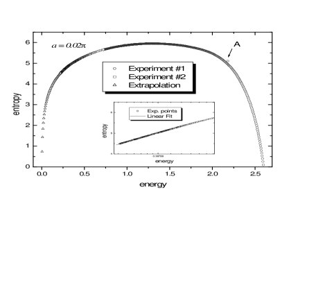
We use the above dynamical criterion to build what we consider as the quasi-stationary sequence $s_{qs}$ versus $\epsilon$, which is shown in FIG.20 by considering $a=0.02\pi$. We obtain the data from two dynamical experiments, as well as by the extrapolation to the low energies region. The first experiment was performed by considering $\mu=0.005$ in order to reduce the rhythm of the dynamical evolution when $\epsilon$ is close to $u_{c}$, and the second one, by considering $\mu=0.1$. The reader can recall that this parameter controls the temporal increase for each computational step, but it does not affect the dependence of distribution function on the energy per particle.

Both experiments were performed by considering $N=20000$ and by dividing the range $0\leq e\leq u_{c}$ in $400$ intervals in order to build the distribution functions. The function $f_{m}\left(e\right)$ was approximated by using a DSIC with $E_{2}=u_{C}$ and $E_{1}=u_{c}-u_{c}/400$. The second experiment starts from a TBIC with $\beta=-10.0$, which exhibits a fast convergence towards the quasi-stationary sequence of the first experiment. Notice that in this figure there is a superposition of both experiments in the intermediate energetic range and no discrepancy is evidenced. The range $0<\epsilon\leq 0.22$ was obtained from the extrapolation of the experimental data because of the evolution is extremely slow in this interval, and basically, the distribution functions do not differ significantly from the truncating Boltzmann profile, yielding $s\simeq 6.035+\ln\epsilon$ in this energetic range.

IV Nonhomogeneous character of the confining potential

The model system considered in the above sections disregards the effect of the nonhomogeneous character of the confining potential energy. We are interested in describing this effect, at least, in the extreme case where the system equilibration mechanism is very effective. As already observed in the numerical experiments, when the particles are able to explore in an effective fashion all those microscopic configurations which are stable under the evaporation, the progressive evolution of the system leads to the setting of the ordinary equilibrium conditions, as an example, the imposition of the detailed balance in the framework of the binary encounters.

In the context of Hamiltonian systems, the equilibration mechanisms relay on the strong chaoticity of the microscopic dynamics. This property usually leads to the ergodicity and the equilibrium conditions are ordinarily described by considering a microcanonical distribution pet . If evaporation is present, the above picture can be naturally generalized by considering a microcanonical distribution where it has been disregarded all those microscopic configurations where the particles are able to escape. The above argument was used in a very recent paper alt in the context of astrophysical systems in order to develop an alternative version of the isothermal model of Antonov antonov .

The stable configurations for a Hamiltonian model of the form:

$$H_{N}=K_{N}+V_{N}=\sum_{k=1}^{N}\frac{1}{2m}\mathbf{p}_{k}^{2}+\sum_{i=1}^{N-1}\sum_{j>i}^{N}\phi\left(\mathbf{r}_{j}-\mathbf{r}_{i}\right),$$ (37)

is the subset of the N-body phase space where the particles satisfy the inequalities: $\mathbf{p}_{k}^{2}/2+u\left(\mathbf{r}_{k}\right)<\epsilon_{S}$, being $\epsilon_{S}$ the energy cutoff, $\mathbf{p}_{k}$ and $u\left(\mathbf{r}_{k}\right)$, the linear momentum and potential energy for the k-th particle:

$$u\left(\mathbf{r}_{k}\right)=\sum_{i\not=k}\phi\left(\mathbf{r}_{k}-\mathbf{r}_{i}\right),$$ (38)

where $k=1,...N$. We are interested in the specific form of the quasi-stationary distribution function $f\left(\mathbf{r},\mathbf{p}\right)$ in such conditions.

This question was solved in ref.alt in the context of astrophysical systems by considering the mean field approximation appearing when $N$ tends to infinity. The generalization of these results is straightforwardly followed by taking into account the generalized form of the mean field potential energy $u\left(\mathbf{r}\right)$:

$$u\left(\mathbf{r}\right)=\int d^{3}\mathbf{x}~{}\phi\left(\mathbf{r-x}\right)\rho\left(\mathbf{x}\right),$$ (39)

where $\rho\left(\mathbf{r}\right)$ is the particles density at the point $\mathbf{r}$ of the physical space. Therefore, we will only expose here the final results. The interested reader can see the ref.alt for details of this analysis in the framework of the Newtonian interaction.

It can be proved that the particles density $\rho\left(\mathbf{r}\right)$ is given by the expression:

$$\rho\left(\mathbf{r}\right)=\left(\frac{m}{2\pi\hbar^{2}\beta}\right)^{\frac{3}{2}}\exp\langle-\mu+C\left(\mathbf{r}\right)-\beta u\left(\mathbf{r}\right)\rangle F\left[\sqrt{\Phi\left(\mathbf{r}\right)}\right],$$ (40)

where $\beta$ and $\mu$ are the canonical parameters which are specified by the energy and particles number constraints, $F\left[z\right]$ is defined by the integral:

$$F\left[z\right]=\pi^{-\frac{3}{2}}\int_{0}^{z}4\pi x^{2}\exp\left(-x^{2}\right)dx,$$ (41)

and $\Phi\left(\mathbf{r}\right)=\beta\left[\epsilon_{S}-u\left(\mathbf{r}\right)\right]$. The function $C\left(\mathbf{r}\right)$ is obtained in a self-consistent way as follows:

$$C\left(\mathbf{r}\right)=\int d^{3}\mathbf{x}~{}\phi\left(\mathbf{r-x}\right)\rho\left(\mathbf{x}\right)\frac{\partial}{\partial u\left(\mathbf{x}\right)}\ln F\left[\sqrt{\Phi\left(\mathbf{x}\right)}\right].$$ (42)

Since $\rho\left(\mathbf{r}\right)=\int d^{3}\mathbf{p}~{}f\left(\mathbf{r},\mathbf{p}\right)$, it is very easy to note that equation (40) is derived from the distribution function $f\left(\mathbf{r},\mathbf{p}\right)$:

$$f\left(\mathbf{r},\mathbf{p}\right)=C_{0}\exp\left(C\left[\mathbf{r}\right)-\beta\epsilon\left(\mathbf{r},\mathbf{p}\right)\right].$$ (43)

which vanishes when $\epsilon\left(\mathbf{r},\mathbf{p}\right)>\epsilon_{S}$, being $\epsilon\left(\mathbf{r},\mathbf{p}\right)=\frac{1}{2m}\mathbf{p}^{2}+u\left(\mathbf{r}\right)$. This expression differs from the truncating isothermal profile only because of the presence of the self-consistent function $C\left(\mathbf{r}\right)$, which appears as an additional consequence of the particle evaporation due to the nonhomogeneous character of the global interaction. Although the $\rho$ versus $u\left(r\right)$ dependence (40) unifies the isothermal with the polytropic dependencies: $\rho\sim\exp\left(C+\Phi\right)$ when $\Phi$ is large enough, while $\rho\sim\exp\left(C\right)\Phi^{\frac{3}{2}}$ when $\Phi<<1$, the presence of the function $C$ introduces a sensitive modification to the features of the solutions.

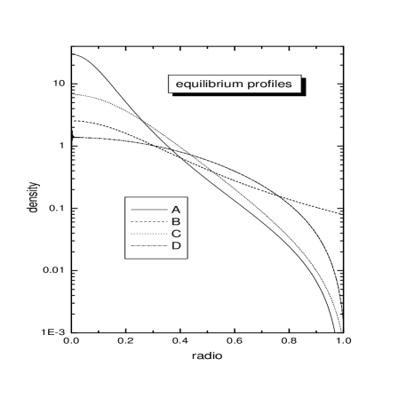
FIG.21 shows the effect of the function $C\left(\mathbf{r}\right)$ in the particles density for the Newtonian potential $\phi\left(r\right)=-\kappa/r$ for configurations with spherical symmetry (details of this study are also found in ref.alt ). The profiles A and C were obtained by considering the distribution function (43): profile A corresponds to a quasi-stationary configuration with low energy, which is characterized by the existence of an isothermal core and a polytropic halo, while C corresponds to a high energy configuration where the isothermal core is not present. Profiles B and D correspond respectively to an isothermal and polytropic configurations with polytropic index $\gamma=\frac{5}{3}$  bin (characterized by the dependence $\rho\left(\Phi\right)\propto\Phi^{\frac{3}{2}}$). The presence of the function $C\left(\mathbf{r}\right)$ leads to a significant concentration of the particles toward the inner regions which goes beyond what the isothermal or the polytropic models predict.

Figure 21: The effect of the function $C\left(\mathbf{r}\right)$ in the particles density for the Newtonian potential.

It is easy to understand that the function $C$ depends in a self-consistent way on the energy function $\epsilon\left(\mathbf{r},\mathbf{p}\right)$. Therefore, the distribution function $f\left(\mathbf{r},\mathbf{p}\right)$, as a whole, depends only on the function $\epsilon\left(\mathbf{r},\mathbf{p}\right)$, that is, $f\left(\mathbf{r},\mathbf{p}\right)=\mathcal{F}\left[\epsilon\left(\mathbf{r},\mathbf{p}\right)\right]$. Needless to say that this is a requirement of the well-known Jeans theorem jeans . However, the consideration of such effect only starting from this last theorem is very unlikely. The present analysis suggests that the simple generalization of the homogeneous distribution functions $f\left(\mathbf{r},\mathbf{p}\right)=\varphi\left(\frac{1}{2m}\mathbf{p}^{2}\right)$, by substituting $\frac{1}{2m}\mathbf{p}^{2}\rightarrow\frac{1}{2m}\mathbf{p}^{2}+u\left(\mathbf{r}\right)$ may be extremely naive, and probably, most of these simple extensions are disregarding important effects of the nonhomogeneous character of the global interaction in presence of particle evaporation.

Thus, the consideration of a weaker chaoticity of the microscopic dynamics and the nonhomogeneous character of the interactions involve serious difficulties in the theoretical prediction of the quasi-stationary profiles. The reader may notice that the approach developed in ref.alt and the standard treatment of some astrophysical structures, such as globular clusters and elliptical galaxies, by using the Michie-King profile king ; bin , are extreme alternatives to consider the effect of the evaporation in such a framework. The applicability of such models depends crucially on how effective is the equilibration mechanism in an actual astrophysical systems.

It is well-established that the picture of the binary encounters provide a nice justification for the use of the King’s models. The basic explanation is found in the fact that the long-range character of the gravitational interaction favors much more the small energy interchange among those distant particles in comparison to the large energy interchanges occurring during the close encounters spitzer ; king ; chandra .

Nevertheless, the binary encounter is not the only equilibration mechanism appearing in this context. In fact, it has been also shown the existence of a very strong chaoticity in gravitational N-body systems pet , which acts in time scales much smaller than the characteristic time for the close binary collisions, as well as it operates for every bound energy. In the viewpoint of the author of such work, this result not only confirms that ”… bound collisionless selfgravitating systems are characterized by a dynamical instability proceeding at a very fast rate, but also suggests that they possess the strongest statistical properties, in analogy with those of standard dynamical systems in the regime of fully developed stochasticity …” pet . As expected, this argument supports the consideration of the ergodic hypothesis in this context, and therefore, the consideration of a suitably regularized microcanonical description for actual astrophysical systems pet ; gross ; de vega ; chava .

Despite the differences concerning to the specific form of the above energy profiles, the question is that the features of their corresponding spatial particle distributions possess more similarities than differences: both distributions lead to finite configurations with isothermal cores and polytropic haloes, even purely polytropic configurations are also possible, where the system size is determined from the tidals interactions.

In the remarkable paper king , King performed a numerical comparison of the Michie-King model with the isothermal distribution truncated at the escape energy, without the consideration of self-consistent function $C$, which is shown in FIG.2 and FIG.7 of this reference. While the King model provides an excellent fit for the data corresponding to a high concentrate globular cluster, the truncated distribution is unable to fit an observational data where a larger concentration of particles appears towards the inner region. In our view, this could be the very effect introduced by taking into consideration the self-consistent function $C$, but this last observation deserves a further analysis. Moreover, it is difficult to distinguish the origin of such effect since there exist other physical backgrounds modifying the form of the particles distribution in the space, such as the mass segregation grif (see also ref.jordan for a recent development).

V Conclusions

The numerical experiments carried out for the gas of binary encounters clearly show the robustness of the quasi-stationary character of the dynamical evolution of this model system. The specific form of the quasi-stationary distribution functions will depend crucially on the effectiveness of the microscopic dynamics in exploring all those microscopic configurations which are stable under the particle evaporation.

An efficient microscopic dynamics leads to the imposition of the detailed balance for all those binary transitions which do not involve particle evaporation, while a decreasing of this effectivity leads to quasi-equilibrium profiles whose specific form depends on the details of the dynamical equations.

The analysis, developed in section IV, in order to take into account the effect of the nonhomogeneous character of the confining interactions for those Hamiltonian systems driven by a strong chaotic dynamics, suggests the appearance of nontrivial effects of the evaporation in the spatial particles distribution. The contribution of such nontrivial effects cause a significant modification of the quasi-stationary profiles, as already shown in the context of the gravitational interaction.

The above results show how difficult could be the theoretical study of the evaporation effect in a general physical background, mainly, when the equilibration mechanisms are not so effective and the dynamics is driven by the presence of long-range forces.