Discrete models of dislocations and their motion in cubic crystals

Abstract

A discrete model describing defects in crystal lattices and having the standard linear anisotropic elasticity as its continuum limit is proposed. The main ingredients entering the model are the elastic stiffness constants of the material and a dimensionless periodic function that restores the translation invariance of the crystal and influences the Peierls stress. Explicit expressions are given for crystals with cubic symmetry: sc, fcc and bcc. Numerical simulations of this model with conservative or damped dynamics illustrate static and moving edge and screw dislocations and describe their cores and profiles. Dislocation loops and dipoles are also numerically observed. Cracks can be created and propagated by applying a sufficient load to a dipole formed by two edge dislocations.

I Introduction

The advances of electronic microscopy allow imaging of atoms and can therefore be used to visualize the core of dislocations nab67 ; hir82 , cracks fre90 and other defects that control crystal growth and the mechanical, optical and electronic properties of the resulting materials science . Emerging behavior due to motion and interaction of defects might explain common but poorly understood phenomena such as friction ger01 . Defects can be created in a controlled way by ion bombardment on reconstructed surfaces RGR01 , which allows the study of effectively two dimensional (2D) single dislocations and dislocation dipoles. These dislocations are effectively 2D because the surface ‘floats’ on the 3D crystal FMS93 . Other defects that are very important in multilayer growth are misfit dislocations MBl74 ; hul01 ; BRB97 . At the nanoscale, many processes (for example, dislocation emission around nanoindentations rojo ) involve the interaction of a few defects so close to each other that their core structure plays a fundamental role. To understand them, the traditional method of using information about the far field of the defects (extracted from linear elasticity) to infer properties of far apart defects reaches its limits. The alternative method of ab initio simulations is very costly and not very practical at the present time. Thus, it would be interesting to have systematic models of defect motion in crystals that can be solved cheaply, are compatible with elasticity and yield useful information about the defect cores and their mobility.

To see what these models of defects might be like, it is convenient to recall a few facts about dislocations. Consider for example an edge dislocation in a simple cubic (sc) lattice with a Burgers vector equal to one interionic distance in gliding motion, as in Fig. 1. The atoms above the $xz$ plane glide over those below. Let us label the atoms by their position before the dislocation moves beyond the origin. Consider the atoms $(x_{0},-a/2,0)$ and $(x_{0},a/2,0)$ which are nearest neighbors before the dislocation passes them. After the passage of the dislocation, the nearest neighbor atoms are $(x_{0},-a/2,0)$ and $(x_{0}-a,a/2,0)$. This large excursion is incompatible with the main assumption under which linear elasticity is derived for a crystal structure ash76 : the deviations of ions in a crystal lattice from their equilibrium positions are small (compared to the interionic distance), and therefore the ionic potentials entering the total potential energy of the crystal are approximately harmonic. One obvious way to describe dislocation motion is to simulate the atomic motion with the full ionic potentials. This description is possibly too costly. In fact, we know that the atomic displacements are small far from the dislocation core and that linear elasticity holds there. Is there an intermediate description that allows dislocation motion in a crystal structure and is compatible with a far field described by the corresponding anisotropic linear elasticity?

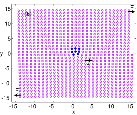
Figure 1: (Color online) Deformed cubic lattice in the presence of an edge dislocation for the piecewise linear $g(x)$ of Eq. (2) with $\alpha=0.24$.

If we try to harmonize the continuum description of dislocations according to elasticity with an discrete description which is simply elasticity with finite differences instead of differentials, we face a second difficulty. The displacement vector of a static edge dislocation is multivalued. For example, its first component is $\tilde{u}_{1}=a(2\pi)^{-1}[\tan^{-1}(y/x)+xy/(2(1-\nu)(x^{2}+y^{2}))]$ for the previously described edge dislocation ($\nu$ is the Poisson ratio) nab67 . In elasticity, this fact does not cause any trouble because the physically relevant strain tensor contains only derivatives of the displacement vector. These derivatives are continuous even across the positive $x$ axis, where the displacement vector has a jump discontinuity $[u_{1}]=a$. If we consider a discrete model, and use differences instead of differentials, the difference of the displacement vector may still have a jump discontinuity across the positive $x$ axis.

The previous difficulties have been solved in a simple discrete model of edge dislocations and crowdions called the IAC model (interacting atomic chains model) proposed and studied by A.I. Landau and collaborators kkl . A similar model for screw dislocations in bcc crystals was proposed earlier by H. Suzuki suzuki . In the equations for the IAC model, the differences of the displacement vector are replaced by their sines. Unlike the finite differences, these sine functions are continuous across the positive $x$ axis. Moreover, the equations remain unchanged if a horizontal chain of atoms slides an integer number of lattice periods $a$ over another chain. Taking advantage of its simplicity, we have recently analyzed pinning and motion of edge dislocations in the IAC model car03 .

In this paper, we propose a top-down approach to discrete models of dislocations in cubic crystals. Let us start with a simple cubic lattice having a unit cell of side length $a$. Firstly, we discretize space along the primitive vectors defining the unit cell of the crystal: $x=x_{1}=la$, $y=x_{2}=ma$, $z=x_{3}=na$, where $l$, $m$ and $n$ are integer numbers. We shall measure the displacement vector in units of $a$, so that $\tilde{u}_{i}(x,y,z,t)=a\,u_{i}(l,m,n;t)$ and $u_{i}(l,m,n;t)$ is a nondimensional vector. Let $D^{+}_{j}$ and $D^{-}_{j}$ represent the standard forward and backward difference operators, so that $D^{\pm}_{1}u_{i}(l,m,n;t)=\pm\,[u_{i}(l\pm 1,m,n;t)-u_{i}(l,m,n;t)]$, and so on. We shall define the discrete distortion tensor as

$$w_{i}^{(j)}=g(D^{+}_{j}u_{i}),$$ (1)

where $g(x)$ is a periodic function of period one satisfying $g(x)\sim x$ as $x\to 0$. In this paper, we shall use the odd continuous piecewise linear function:

$$g(x)=\left\{\begin{array}[]{ll}x,\quad|x|<{1\over 2}-\alpha,\\ {(1-2\alpha)(1-2x)\over 4\alpha}\,,\quad{1\over 2}-\alpha<x<{1\over 2},\end{array}\right.$$ (2)

which is periodically extended outside the interval $(-1/2,1/2)$ for a given $\alpha$, $0<\alpha<1/2$. Note that $g(x)$ is symmetrical if $\alpha=1/4$ and that the interval of $x$ in which $g^{\prime}(x)<0$ widens with respect to that in which $g^{\prime}(x)>0$ as $\alpha$ increases. Numerical simulations of the governing equations for a 2D edge dislocation show that the Peierls stress decreases as $\alpha$ increases; see Fig. 2, which will be further commented later on. This means that the dislocation is harder to move if $\alpha$ decreases, i.e., if the interval of $x$ in which $g^{\prime}(x)<0$ shrinks with respect to that in which $g^{\prime}(x)>0$. The parameter $\alpha$ can be selected so as to agree with the observed or calculated Peierls stress of a given crystal.

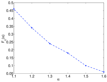
Figure 2: (Color online) Peierls stress in dimensionless units for a 2D edge dislocation in a sc crystal with the stiffnesses of tungsten as a function of the parameter $\alpha$ in the periodic function $g(x)$.

Secondly, we replace the strain tensor in the strain energy by

$$e_{ij}={1\over 2}\,(w_{i}^{(j)}+w_{j}^{(i)})={g(D^{+}_{j}u_{i})+g(D^{+}_{i}u_{j})\over 2}.$$ (3)

Summing the strain energy over all lattice sites, we obtain the potential energy of the crystal:

$$V(\{u_{i}\}) = a^{3}\,\sum_{l,m,n}W(l,m,n;t).$$ (4)

$$W(l,m,n;t) = W(\{u_{i}\})={1\over 2}c_{ijkl}e_{ij}e_{kl},$$ (5)

$$c_{ijkl} = \lambda\,\delta_{ij}\delta_{kl}+\mu\,(\delta_{ik}\delta_{jl}+\delta_{il}\delta_{jk})+2(C_{44}-\mu)$$ (6)

$$\times \left({\delta_{ik}\delta_{jl}+\delta_{il}\delta_{jk}\over 2}-\delta_{1i}\delta_{1j}\delta_{1k}\delta_{1l}-\delta_{2i}\delta_{2j}\delta_{2k}\delta_{2l}-\delta_{3i}\delta_{3j}\delta_{3k}\delta_{3l}\right),$$

in which summation over repeated indices is understood. Here, $\lambda=C_{12}$, $\mu=(C_{11}-C_{12})/2$, where $C_{ij}$ are the stiffness constants of a cubic crystal. If $C_{44}=\mu$, the strain energy is isotropic and $\lambda$ and $\mu$ are the usual Lamé coefficients.

Next, we find the equations of motion. In the absence of dissipation and fluctuation effects, they are

$$\rho a^{4}\,\ddot{u}_{i}(l,m,n;t)=-{1\over a}\,{\partial V(\{u_{k}\})\over\partial u_{i}(l,m,n;t)},$$ (7)

or, equivalently,

$$M\,\ddot{u}_{i}(l,m,n;t) = -{\partial\over\partial u_{i}(l,m,n;t)}\sum_{l^{\prime},m^{\prime},n^{\prime}}W(l^{\prime},m^{\prime},n^{\prime};t),$$ (8)

$$M = \rho a^{2}.$$ (9)

Here $\ddot{u}_{i}\equiv\partial^{2}u_{i}/\partial t^{2}$, $M$ has units of mass per unit length (because $\rho$ is the mass density) and the displacement vector is dimensionless, so that both sides of Eq. (8) have units of force per unit area. We show in Appendix A that Eq. (8) is equivalent to the following spatially discrete equations

$$M\,\ddot{u}_{i} = \sum_{j,k,l}D^{-}_{j}[c_{ijkl}\,g^{\prime}(D^{+}_{j}u_{i})\,g(D^{+}_{l}u_{k})].$$ (10)

To nondimensionalize these equations, we could adopt $C_{44}$ as the typical scale of stress and $t_{0}=\sqrt{M/C_{44}}=a\sqrt{\rho/C_{44}}$ as the time scale. The resulting equations are the same ones with $M=1$ and $c_{ijkl}/C_{44}$ instead of $c_{ijkl}$. Let us now restore dimensional units to this equation, so that $\tilde{u}_{i}(x,y,z)=a\,u_{i}(x/a,y/a,z/a)$, then let $a\to 0$, use Eq. (9) and that $g(x)\sim x$ as $x\to 0$. Then we obtain the equations of linear elasticity ll7 ,

$$\rho\,{\partial^{2}\tilde{u}_{i}\over\partial t^{2}}=\sum_{j,k,l}{\partial\over\partial x_{j}}\left(c_{ijkl}\,{\partial\tilde{u}_{k}\over\partial x_{l}}\right).$$ (11)

Thus the discrete model with conservative dynamics yields the Cauchy equations for elastic constants with cubic symmetry provided the components of the distortion tensor are very small (which holds in the dislocation far field). Equations of motion with dissipation and fluctuation terms can be obtained by writing a quadratic dissipative function which, in the isotropic case, yields the usual fluid viscosity terms and using the fluctuation-dissipation theorem unpub .

In the rest of the paper, we describe dislocation motion in simple cubic crystals and extend our discrete elastic equations to the case of fcc and bcc lattices.

II Dislocation motion in sc crystals

In this Section, we shall find numerically pure screw and edge dislocations of our discrete model for sc symmetry and discuss their motion under appropriate applied stresses. In all cases, the procedure to obtain numerically the dislocation from the discrete model equations is the same. We first solve the stationary equations of continuum elasticity with appropriate singular source terms to obtain the dimensional displacement vector ${\bf\tilde{u}}(x,y,z)=(\tilde{u}_{1}(x,y,z),\tilde{u}_{2}(x,y,z),\tilde{u}_{3}(x,y,z))$ of the static dislocation under zero applied stress. This displacement vector yields the far field of the corresponding dislocation for the discrete model, which is the nondimensional displacement vector: ${\bf U}(l,m,n)={\bf\tilde{u}}(la,ma,na)/a$. We use the nondimensional static displacement vector ${\bf U}(l,m,n)$ in the boundary and initial conditions for the discrete equations of motion of the discrete model. Later in the Section, we shall show numerical results corresponding to the interaction of edge dislocations and the opening of a crack.

II.1 Screw dislocations

Figure 3: (Color online) Screw dislocation for the piecewise linear $g(x)$ of Eq. (2) with $\alpha=0.24$.

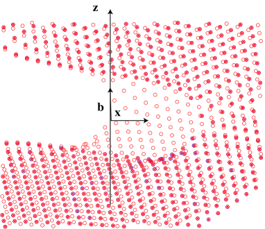
Figure 4: (Color online) Superimposed zooms of the moving core of a screw dislocation.

The continuum displacement field of a dislocation, ${\bf\tilde{u}}=(\tilde{u}_{1},\tilde{u}_{2},\tilde{u}_{3})$, can be calculated as a stationary solution of the anisotropic Navier equations with a singularity $\propto r^{-1}$ at the dislocation core and such that $\int_{\mathcal{C}}(d{\bf x}\cdot\nabla){\bf\tilde{u}}=-{\bf b}$, where ${\bf b}$ is the Burgers vector and $\mathcal{C}$ is any closed curve encircling the dislocation line ll7 . A pure screw dislocation along the $z$ axis with Burgers vector ${\bf b}=(0,0,b)$ has a displacement vector ${\bf\tilde{u}}=(0,0,\tilde{u}_{3}(x,y))$ nab67 . Then the strain energy density (5) becomes $W=C_{44}\,|\nabla\tilde{u}_{3}|^{2}/2$, and the stationary equation of motion is $\Delta\tilde{u}_{3}=0$. Its solution corresponding to a screw dislocation is $\tilde{u}_{3}(x,y)=b\,(2\pi)^{-1}\tan^{-1}(y/x)$ nab67 . The same symmetry considerations for Eq. (10) yield the following discrete equation for the $z$ component of the nondimensional displacement $u_{3}(l,m;t)$:

$$M\,\ddot{u_{3}} = C_{44}\,\{D^{-}_{1}[g(D^{+}_{1}u_{3})\,g^{\prime}(D^{+}_{1}u_{3})]+D^{-}_{2}[g(D^{+}_{2}u_{3})\,g^{\prime}(D^{+}_{2}u_{3})]\}.$$ (12)

Numerical solutions of Eq. (12) show that a static screw dislocation moves if an applied shear stress surpasses the static Peierls stress, $|F|>F_{cs}$, but that a moving dislocations continues doing so until the applied shear stress falls below a lower threshold $F_{cd}$ (dynamic Peierls stress); see Ref. car03 for a similar situation for edge dislocations. To find the static solution of this equation corresponding to a screw dislocation, we could minimize an energy functional. However, it is more efficient to solve the following overdamped equation:

$$\beta\,\dot{u_{3}} = C_{44}\,\{D^{-}_{1}[g(D^{+}_{1}u_{3})\,g^{\prime}(D^{+}_{1}u_{3})]+D^{-}_{2}[g(D^{+}_{2}u_{3})\,g^{\prime}(D^{+}_{2}u_{3})]\}.$$ (13)

The stationary solutions of Eqs. (12) and (13) are the same, but the solutions of (13) relax rapidly to the stationary solutions if we choose appropriately the damping coefficient $\beta$. We solve Eq. (13) with initial condition $u_{3}(l,m;0)=U_{3}(l,m)\equiv b\,(2\pi a)^{-1}\tan^{-1}(m/l)$, and with boundary conditions $u_{3}(l,m;t)=U_{3}(l,m)+F\,m$ at the upper and lower boundaries of our lattice. At the lateral boundaries, we use zero-flux Neumann boundary conditions. Here $F$ is an applied dimensionless stress with $|F|<F_{cs}$; to obtain the dimensional stress we should multiply $F$ by $C_{44}$. For such small stress, the solution of Eq. (13) relaxes to a static screw dislocation $u_{3}(l,m)$ with the desired far field. If $F=0$, Figure 3 shows the helical structure adopted by the deformed lattice $(l,m,n+u_{3}(l,m))$ for the piecewise linear $g(x)$ of Eq. (2) with $\alpha=0.24$. The numerical solution shows that moving a dislocation requires that we should have $g^{\prime}(D_{j}^{+}u_{3})<0$ (with either $j=1$ or 2) in (12) or (13) at its core car03 . This is harder to achieve as $\alpha$ decreases.

The motion of a pure screw dislocation is somewhat special because its Burgers vector is parallel to the dislocation line. Any plane containing the Burgers vector can be a glide plane. Under a shear stress $F>F_{cs}$ directed along the $y$ direction, a screw dislocation moves on the glide plane $xz$. A moving screw dislocation has the structure of a discrete traveling wave in the direction $x$, with far field $u_{3}(l-ct,m)+Fm$; $c=c(F)$ is the dislocation speed; see Figure 4. This is similar to the case of edge dislocations in the simple IAC model kkl , as discussed in car03 where the details of the analysis can be looked up.

II.2 Edge dislocations

To analyze edge dislocations in the simplest case, we consider a isotropic cubic crystal ($C_{44}=(C_{11}-C_{12})/2$) with planar discrete symmetry, so that ${\bf u}(l,m;t)=(u_{1}(l,m;t),u_{2}(l,m;t),0)$ is independent of $z=na$.

To find the stationary edge dislocation of the discrete model, we first have to write the corresponding stationary edge dislocation of isotropic elasticity. An edge dislocation directed along the $z$ axis (dislocation line), and having Burgers vector $(b,0,0)$ has a displacement vector ${\bf\tilde{u}}=(\tilde{u}_{1}(x,y),\tilde{u}_{2}(x,y),0)$ with a singularity $\propto r^{-1}$ at the core and satisfying $\int_{\mathcal{C}}(d{\bf x}\cdot\nabla){\bf\tilde{u}}=-(b,0,0)$, for any closed curve $\mathcal{C}$ encircling the $z$ axis. It satisfies the planar stationary Navier equations with a singular source term:

$$\Delta{\bf\tilde{u}}+{1\over 1-2\nu}\nabla(\nabla\cdot{\bf\tilde{u}})=-(0,b,0)\,\delta(r).$$ (14)

Here $r=\sqrt{x^{2}+y^{2}}$ and $\nu=\lambda/[2(\lambda+\mu)]$ is the Poisson ratio; cf. page 114 of Ref. ll7 . The appropriate solution is

$$\tilde{u}_{1} = {b\over 2\pi}\left[\tan^{-1}\left({y\over x}\right)+{xy\over 2(1-\nu)(x^{2}+y^{2})}\right],$$

$$\tilde{u}_{2} = {b\over 2\pi}\left[-{1-2\nu\over 4(1-\nu)}\,\ln\left({x^{2}+y^{2}\over b^{2}}\right)+{y^{2}\over 2(1-\nu)(x^{2}+y^{2})}\right],$$ (15)

cf. Ref. nab67 , pag. 57.

Eqs. (15) yield the nondimensional static displacement vector ${\bf U}(l,m)=(\tilde{u}_{1}(la,ma)/a,\tilde{u}_{2}(la,ma)/a,0)$, which will be used to find the stationary edge dislocation of the discrete equations of motion. For this planar configuration, the conservative equations of motion (10) become

$$M\,\ddot{u}_{1} = C_{11}\,D^{-}_{1}[g(D^{+}_{1}u_{1})\,g^{\prime}(D^{+}_{1}u_{1})]+C_{12}\,D^{-}_{1}[g(D^{+}_{2}u_{2})\,g^{\prime}(D^{+}_{1}u_{1})]$$ (16)

$$+C_{44}\,D^{-}_{2}\{[g(D^{+}_{2}u_{1})+g(D^{+}_{1}u_{2})]\,g^{\prime}(D^{+}_{2}u_{1})\},$$

$$M\,\ddot{u}_{2} = C_{11}\,D^{-}_{2}[g(D^{+}_{2}u_{2})\,g^{\prime}(D^{+}_{2}u_{2})]+C_{12}\,D^{-}_{2}[g(D^{+}_{1}u_{1})\,g^{\prime}(D^{+}_{2}u_{2})]$$ (17)

$$+C_{44}\,D^{-}_{1}\{[g(D^{+}_{1}u_{2})+g(D^{+}_{2}u_{1})]\,g^{\prime}(D^{+}_{1}u_{2})\}.$$

To find the stationary edge dislocation corresponding to these equations, we set $C_{44}=(C_{11}-C_{12})/2$ (isotropic case), and replace the inertial terms $M\ddot{u}_{1}$ and $M\ddot{u}_{2}$ by $\beta\dot{u}_{1}$ and $\beta\dot{u}_{2}$, respectively. The resulting overdamped equations,

$$\beta\,\dot{u}_{1} = C_{11}\,D^{-}_{1}[g(D^{+}_{1}u_{1})\,g^{\prime}(D^{+}_{1}u_{1})]+C_{12}\,D^{-}_{1}[g(D^{+}_{2}u_{2})\,g^{\prime}(D^{+}_{1}u_{1})]$$ (18)

$$+C_{44}\,D^{-}_{2}\{[g(D^{+}_{2}u_{1})+g(D^{+}_{1}u_{2})]\,g^{\prime}(D^{+}_{2}u_{1})\},$$

$$\beta\,\dot{u}_{2} = C_{11}\,D^{-}_{2}[g(D^{+}_{2}u_{2})\,g^{\prime}(D^{+}_{2}u_{2})]+C_{12}\,D^{-}_{2}[g(D^{+}_{1}u_{1})\,g^{\prime}(D^{+}_{2}u_{2})]$$ (19)

$$+C_{44}\,D^{-}_{1}\{[g(D^{+}_{1}u_{2})+g(D^{+}_{2}u_{1})]\,g^{\prime}(D^{+}_{1}u_{2})\},$$

have the same stationary solutions as Eqs. (16) and (17). We solve Eqs. (18) and (19) with initial condition ${\bf u}(l,m;0)={\bf U}(l,m)$ given by Eqs. (15), and with boundary conditions ${\bf u}(l,m;t)={\bf U}(l,m)+(F\,m,0,0)$ at the upper and lower boundaries of the lattice ($F$ is a dimensionless applied shear stress; recall that the displacement vector in the discrete equations is always dimensionless). If $|F|<F_{cs}$ ($F_{cs}$ is the static Peierls stress for edge dislocations), the solution of Eqs. (18) and (19) relaxes to a static edge dislocation $(u_{1}(l,m),u_{2}(l,m),0)$ with the appropriate continuum far field.

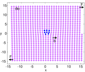
Figure 5: (Color online) Edge dislocation for the piecewise linear $g(x)$ of Eq. (2) with (a) $\alpha=0.27$, (b) $\alpha=0.29$, (c) $\alpha=0.32$.

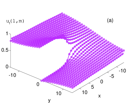
Figure 6: (Color online) Profile of $u_{1}(l,m)$ for an edge dislocation with the piecewise linear $g(x)$ of Eq. (2) when (a) $\alpha=0.24$, (b) $\alpha=0.32$.

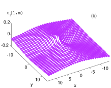
Figure 7: (Color online) Profile of $u_{2}(l,m)$ for an edge dislocation with the piecewise linear $g(x)$ of Eq. (2) when (a) $\alpha=0.24$, (b) $\alpha=0.27$, (c) $\alpha=0.29$, (d) $\alpha=0.32$.

In our numerical calculations of the static edge dislocation, we use the elastic constants of tungsten (which is an isotropic bcc crystal), $C_{11}=521$ GPa, $C_{12}=201$ GPa, $C_{44}=160$ GPa ($C_{11}=C_{12}+2C_{44}$) hir82 . This yields $\nu=0.278$. Figure 5 shows the structure adopted by the deformed lattice $(l+u_{1}(l,m),m+u_{2}(l,m))$ when $\nu=0.278$. for the asymmetric piecewise linear function $g(x)$ with three different values of $\alpha$. The profiles of the displacement vector are shown in Figures 6 and 7. The glide motion of edge dislocations occurs on the glide plane defined by their Burgers vector and the dislocation line, and in the direction of the Burgers vector. In our case, a shear stress in the direction $y$, will move the dislocation in the direction $x$. For conservative or damped dynamics, the applied shear stress has to surpass the static Peierls stress to depin a static dislocation, and a moving dislocation propagates provided the applied stress is larger than the dynamic Peierls stress (smaller than the static one) car03 . Numerical solutions show that the dimensionless Peierls stress depends on $\alpha$ in Eq. (2) as shown in Fig. 2. As the interval of $x$ for which $g^{\prime}(x)<0$ shrinks (which occurs as $\alpha$ decreases), the static Peierls stress increases and the dislocation becomes harder to move. The size of the dislocation core is also related to the shape of $g(x)$. As shown by Figures 5 to 7, the dislocation core expands as $\alpha$ increases: for $\alpha\leq 0.26$, the dislocation core is very narrow, as shown in Figs. 5(a) and 7(a). Figs. 5(b), and 7(a) to 7(c) show that the dislocation core widens one lattice point as $\alpha$ sweep the interval $0.26<\alpha<0.29$, in which the variation of the Peierls stress is very small (see the plateau in Fig. 2). The dislocation core gains more lattice points as $\alpha$ increases to 0.32 and beyond, cf. Figs. 5(c), 6(b) and 7(d). Thus the size of the dislocation core and the Peierls stress are related to the width of the interval of $x$ for which $g^{\prime}(x)<0$ and to the actual value of the slope. As an additional example, the symmetric sine function $g(x)=\sin(2\pi x)/(2\pi)$ has wide subintervals of small slope, which produces very low Peierls stresses and an artificially wide dislocation core. In kkl ; car03 , this problem was avoided by setting $u_{2}=0$ and changing $g(D^{+}_{1}u_{1})\leftrightarrow D^{+}_{1}u_{1}$ and $2\pi g(D^{+}_{2}u_{1})=\sin(2\pi D^{+}_{1}u_{1})$ in (16) and (18). A moving dislocation is a discrete traveling wave advancing along the $x$ axis, and having far field $(u_{1}(l-ct,m)+Fm,u_{2}(l-ct,m))$. The analysis of depinning and motion of planar edge dislocations follows that explained in Ref. car03 with technical complications due to our more complex discrete model.

II.3 Interaction of edge dislocations and crack formation

The reduced 2D model (16) - (17) can be solved numerically to illustrate interaction of edge dislocations. Figure 8 illustrates the repulsion of equal-sign edge dislocations whereas opposite edge dislocations attract each other and form dislocation loops as in Fig. 9 or dislocation dipoles as in Fig. 10. Friction terms affect numerical simulations of the model as follows. As in the case of 1D models wavy , atoms may oscillate far from the core of a moving dislocation when the equations of motion are conservative or slightly damped. Large friction (order one coefficients) reduces the oscillations of individual atoms, the instantaneous position of the core of the defect is easier to locate and its movement in the distorted lattice is easier to follow. Small friction (order $10^{-2}$ coefficients) results in dislocation glide combined with oscillations of the individual atoms. The figures 8, 9 and 10 were obtained with small friction. See Refs. wavy, and carPRL01, on the impact of friction and inertia on 1D wave front profiles.

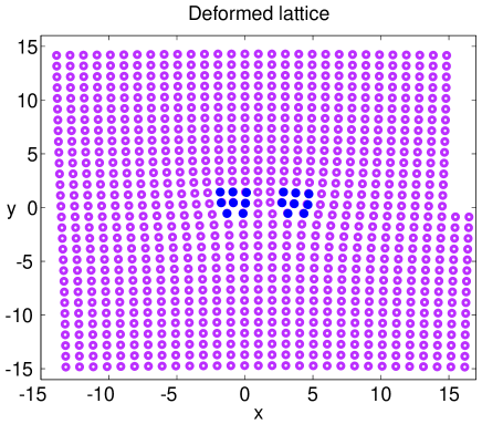
Figure 8: (Color online) Repulsion of like sign edge dislocations.

Figure 9: (Color online) Atraction of opposite sign edge dislocations leading to formation of a dislocation loop.

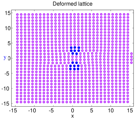
Figure 10: (Color online) Atraction of opposite sign edge dislocations leading to formation of a dislocation dipole.

Figure 11 shows the formation of a crack propagating in the $x$ direction under an applied tension in the $y$ direction. In principle, numerically solving the discrete equations of motion we can find: (i) the threshold stress for crack propagation, (ii) the direction of propagation, (iii) the crack speed, and (iv) the crack shape. We do not need to impose additional conditions such as displacement thresholds for breaking atomic bonds as in the usual spring models for brittle fracture sle81 ; guinea .

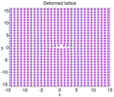
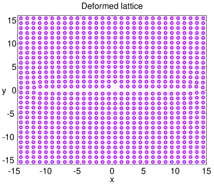
Figure 11: (Color online) Snapshots showing crack generation and growth induced by applying a tension in the direction $y$ to a dislocation dipole.

III Elasticity in a non-orthogonal basis

III.1 Equations of motion

For fcc or bcc crystals, the primitive vectors of the unit cell are not orthogonal. To find a discrete model for these crystals, we should start by writing the strain energy density in a non-orthogonal vector basis, $a_{1}$, $a_{2}$, $a_{3}$, in terms of the usual orthonormal vector basis $e_{1}$, $e_{2}$, $e_{3}$ determined by the cube sides of length $a$. Let $x_{i}$ denote coordinates in the basis $e_{i}$, and let $x^{\prime}_{i}$ denote coordinates in the basis $a_{i}$. Notice that the $x_{i}$ have dimensions of length while the $x^{\prime}_{i}$ are dimensionless. The matrix $T=(a_{1},a_{2},a_{3})$ whose columns are the coordinates of the new basis vectors in terms of the old orthonormal basis can be used to change coordinates as follows:

$$x_{i}^{\prime}=T_{ij}^{-1}x_{j},\;x_{i}=T_{ij}x^{\prime}_{j}.$$ (20)

Similarly, the displacement vectors in both basis are related by

$$u_{i}^{\prime}=T_{ij}^{-1}u_{j},\;u_{i}=T_{ij}u^{\prime}_{j},$$ (21)

and partial derivatives obey

$${\partial\over\partial x_{i}^{\prime}}=T_{ji}{\partial\over\partial x_{j}},\;{\partial\over\partial x_{i}}=T_{ji}^{-1}{\partial\over\partial x_{j}^{\prime}}.$$ (22)

By using these equations, the strain energy density $W=(1/2)c_{iklm}e_{ik}e_{lm}$ can be written as

$$W={1\over 2}\,c_{ijlm}{\partial u_{i}\over\partial x_{j}}{\partial u_{l}\over\partial x_{m}}={1\over 2}\,c_{rspq}^{\prime}{\partial u_{r}^{\prime}\over\partial x_{s}^{\prime}}{\partial u_{p}^{\prime}\over\partial x_{q}^{\prime}},$$ (23)

where the new elastic constants are:

$$c_{rspq}^{\prime}=c_{ijlm}T_{ir}T_{sj}^{-1}T_{lp}T_{qm}^{-1}.$$ (24)

Notice that the elastic constants have the same dimensions in both the orthogonal and the non-orthogonal basis. To obtain a discrete model, we shall consider that the dimensionless displacement vector $u^{\prime}_{i}$ depends on dimensionless coordinates $x^{\prime}_{i}$ that are integer numbers $u^{\prime}_{i}=u^{\prime}_{i}(l,m,n;t)$. As in the case of sc crystals, we replace the distortion tensor (gradient of the displacement vector in the non-orthogonal basis) by a periodic function of the corresponding forward difference, $w_{i}^{(j)}=g(D^{+}_{j}u^{\prime}_{i})$, cf. Eq. (2). The discretized strain energy density is

$$W(l,m,n;t)={1\over 2}\,c_{rspq}^{\prime}g(D^{+}_{s}u_{r}^{\prime})\,g(D^{+}_{q}u_{p}^{\prime}).$$ (25)

The elastic constants $c_{rspq}^{\prime}$ can be calculated in terms of the Voigt stiffness constants for a cubic crystal, $C_{11}$, $C_{44}$ and $C_{12}$. Eq. (6) yields $c_{ijlm}=C_{44}(\delta_{il}\delta_{jm}+\delta_{im}\delta_{lj})+C_{12}\delta_{ij}\delta_{lm}-H(\delta_{1i}\delta_{1j}\delta_{1l}\delta_{1m}+\delta_{2i}\delta_{2j}\delta_{2l}\delta_{2m}+\delta_{3i}\delta_{3j}\delta_{3l}\delta_{3m})$, where $H=2C_{44}+C_{12}-C_{11}$ measures the anisotropy of the crystal and Eq. (24) provides the tensor $c_{rspq}^{\prime}$. The elastic energy can be obtained from Eq. (25) for $W$ by means of Eqs. (4). Then the equations of motion (7) are

$$\rho a^{3}\,{\partial^{2}u^{\prime}_{i}\over\partial t^{2}}=-T^{-1}_{iq}T_{pq}^{-1}{\partial V\over\partial u_{p}^{\prime}},$$

which, together with Eqs. (4) and (25), yield

$$\rho\,{\partial^{2}u^{\prime}_{i}\over\partial t^{2}}=T^{-1}_{iq}T_{pq}^{-1}\,D^{-}_{j}[c_{pjrs}^{\prime}\,g^{\prime}(D^{+}_{j}u_{p}^{\prime})\,g(D^{+}_{s}u_{r}^{\prime})].$$ (26)

This equation becomes (10) for orthogonal coordinates, $T^{-1}_{iq}=\delta_{iq}/a$, once we take into account the Einstein convention on summation over repeated indices in (10).

III.2 Far field of a dislocation

As in the case of sc crystals studied in Section II, we should determine the elastic far field of a dislocation under zero stress to set up the initial and boundary data needed to solve numerically the discrete equations of motion (26). We can calculate the elastic far field of any straight dislocation following the method explained in Chapter 13 of Hirth and Lothe’s book hir82 . Firstly, we determine the elastic constants in an orthonormal coordinate system $e_{1}^{\prime\prime}$, $e_{2}^{\prime\prime}$, $e_{3}^{\prime\prime}$ with $e_{3}^{\prime\prime}=-\xi$ parallel to the dislocation line. The result is

$$c_{ijkl}^{\prime\prime}=c_{ijkl}-H\sum_{n=1}^{3}(S_{in}S_{jn}S_{kn}S_{ln}-\delta_{in}\delta_{jn}\delta_{kn}\delta_{ln}).$$ (27)

Here the rows of the orthogonal matrix $S=(e_{1}^{\prime\prime},e_{2}^{\prime\prime},e_{3}^{\prime\prime})^{t}$ are the coordinates of the $e_{i}^{\prime\prime}$’s in the old orthonormal basis $e_{1}$, $e_{2}$, $e_{3}$. In these new coordinates, the elastic displacement field $(u_{1}^{\prime\prime},u_{2}^{\prime\prime},u_{3}^{\prime\prime})$ depends only on $x_{1}^{\prime\prime}$ and on $x_{2}^{\prime\prime}$. The Burgers vector and the elastic displacement field satisfy $b^{\prime\prime}_{1}=b^{\prime\prime}_{2}=0$ and $u_{1}^{\prime\prime}=u_{2}^{\prime\prime}=0$ for a pure screw dislocation in an infinite medium. For a pure edge dislocation, $b^{\prime\prime}_{3}=0$ and $u_{3}^{\prime\prime}=0$. Secondly, the displacement vector $(u_{1}^{\prime\prime},u_{2}^{\prime\prime},u_{3}^{\prime\prime})$ is calculated as follows:

• Select three roots $p_{1},p_{2},p_{3}$ with positive imaginary part out of each pair of complex conjugate roots of the polynomial $det[a_{ik}(p)]=0$, $a_{ik}(p)=c_{i1k1}^{\prime\prime}+(c_{i1k2}^{\prime\prime}+c_{i2k1}^{\prime\prime})p+c^{\prime\prime}_{i2k2}p^{2}$.

• For each $n=1,2,3$ find an eigenvector $A_{k}(n)$ associated to the zero eigenvalue for the matrix $a_{ik}(p_{n})$.

• Solve Re$\sum_{n=1}^{3}A_{k}(n)D(n)=b^{\prime\prime}_{k},$ $k=1,2,3$ and Re$\sum_{n=1}^{3}\sum_{k=1}^{3}(c^{\prime\prime}_{i2k1}+c^{\prime\prime}_{i2k2}p_{n})A_{k}(n)D(n)=0$, $i=1,2,3$ for the imaginary and real parts of $D(1)$,$D(2)$,$D(3)$.

• For $k=1,2,3$, $u_{k}^{\prime\prime}=$ Re$[-{1\over 2\pi i}\sum_{n=1}^{3}A_{k}(n)D(n)\ln(x_{1}^{\prime\prime}+p_{n}x_{2}^{\prime\prime})]$.

Lastly, we can calculate the displacement vector $u_{k}^{\prime}$ in the non-orthogonal basis $a_{i}$ from $u_{k}^{\prime\prime}$.

III.3 Discrete models for fcc metals

For fcc metals, the non-orthogonal vector basis comprising primitive vectors is

$$a_{1}={a\over 2}\,(1,1,0),\;a_{2}={a\over 2}\,(0,1,1),\;a_{3}={a\over 2}\,(1,0,1).$$ (28)

The equations of motion are (26) with the corresponding transformation matrix $T=(a_{1},a_{2},a_{3})$.

We shall now analyze the motion of dislocations in the case of gold. The initial and boundary data for the numerical simulations are constructed from the far fields of dislocations in anisotropic elasticity as explained in the previous Subsection. We have considered two straight dislocations: the perfect edge dislocation directed along $\xi=(-1,1,-2)/\sqrt{6}$ (with a Burgers vector which is one of the translation vectors of the lattice, and therefore glide of the dislocation leaves behind a perfect crystal hul01 ) and the pure screw dislocation along $\xi=(1,1,0)/\sqrt{2}$. For the perfect edge dislocation, we select:

$$e_{1}^{\prime\prime}=(-1,-1,0)/\sqrt{2},\;e_{2}^{\prime\prime}=(1,-1,-1)/\sqrt{3},\;e_{3}^{\prime\prime}=(1,-1,2)/\sqrt{6},$$ (29)

which are unit vectors parallel to the Burgers vector ${\bf b}$, the normal to the glide plane ${\bf n}$, and minus the tangent to the dislocation line $-\xi$, respectively. For the pure screw dislocation, we have:

$$e_{1}^{\prime\prime}=(1,-1,2)/\sqrt{6},\;e_{2}^{\prime\prime}=(-1,1,1)/\sqrt{3},\;e_{3}^{\prime\prime}=(-1,-1,0)/\sqrt{2},$$ (30)

where $e_{2}^{\prime\prime}$ is a unit vector normal to the glide plane and $e_{3}^{\prime\prime}$ is a unit vector parallel to the dislocation line and to the Burgers vector (but directed in the opposite sense).

For gold, $C_{11}=186$ GPa, $C_{44}=42$ GPa, $C_{12}=157$ GPa and $H=55$ GPa. The lattice constant is $a=4.08$ Å  and the density is $\rho=1.74$ g/cm³. Figures 12 and 13 show the perfect edge dislocation and the screw dislocation obtained as stationary solutions of model (26). Due to the boundary conditions we have chosen, their far fields match the corresponding elastic far fields of the dislocations (written in the non-orthogonal coordinates corresponding to the primitive cell vectors $a_{1}$, $a_{2}$, $a_{3}$). Dark and light colors are used to trace points placed in different planes in the original lattice. Note that the planes perpendicular to the Burgers vector in Fig. 12 have a two-fold stacking sequence ‘dark-light-dark-light …’ The extra half-plane of the edge dislocation consists of two half planes (one dark and one light) in the dark-light-dark-light …  sequence. Movement of this unit dislocation by glide retains continuity of the dark planes and the light planes across the glide plane, except at the dislocation core where the extra half planes terminate hul01 .

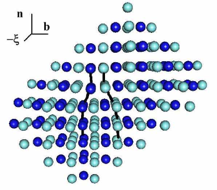
Figure 12: (Color online) Perfect edge dislocation in a gold lattice displaying a two-fold stacking sequence of planes. Lines locating the dislocation core are a guide for the eye.

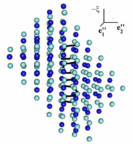
Figure 13: (Color online) Screw dislocation in a gold lattice. Lines locating the dislocation core are a guide for the eye.

III.4 Discrete models for bcc metals

The discrete model for bcc metals is similar to that for fcc metals explained in the previous Subsection, but the non-orthogonal vector basis comprising primitive vectors is now

$$a_{1}={a\over 2}\,(1,1,1),\;a_{2}={a\over 2}\,(-1,1,1),\;a_{3}={a\over 2}\,(1,-1,1).$$ (31)

The equations of motion are (26) with the corresponding transformation matrix $T=(a_{1},a_{2},a_{3})$.

As in the previous Subsection, we calculate the elastic displacements of an edge dislocation and a screw dislocation in iron. For the edge dislocation we select:

$$e_{1}^{\prime\prime}=(1,1,1)/\sqrt{3},\;e_{2}^{\prime\prime}=(-1,0,1)/\sqrt{2},\;e_{3}^{\prime\prime}=(1,-2,1)/\sqrt{6},$$ (32)

which are unit vectors in the directions of the Burgers vector ${\bf b}$, the normal to the glide plane ${\bf n}$ and the dislocation line vector, respectively. For the pure screw dislocation:

$$e_{1}^{\prime\prime}=(-1,0,1)/\sqrt{2},\;e_{2}^{\prime\prime}=(-1,2,-1)/\sqrt{6},\;e_{3}^{\prime\prime}=-(1,1,1)/\sqrt{3}$$ (33)

where $e_{2}^{\prime\prime}$ is the normal to the glide plane and $e_{3}^{\prime\prime}$ a unit vector parallel to the dislocation line and to the Burgers vector.

For iron, $C_{11}=242$ GPa, $C_{44}=112$ GPa, $C_{12}=146.5$ GPa and $H=129$ GPa. The lattice constant is $a=2.87$ Å  and the density $\rho=7.86$ g/cm³. Figures 14 and 15 show the edge and the screw dislocations obtained as stationary solutions of model (26). Their far fields match the corresponding elastic far fields of the dislocations (written in the non-orthogonal coordinates corresponding to the primitive cell vectors $a_{1}$, $a_{2}$, $a_{3}$). Dark and ligh colors are used to trace points placed initially in different planes perpendicular to the Burgers vector.

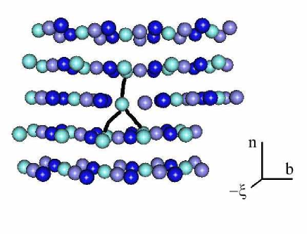
Figure 14: (Color online) Edge dislocation in an iron lattice. Lines locating the dislocation core are a guide for the eye.

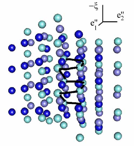
Figure 15: (Color online) Screw dislocation in an iron lattice. Lines locating the dislocation core are a guide for the eye.

IV Conclusions

We have proposed discrete models describing defects in crystal structures whose continuum limit is the standard linear anisotropic elasticity. The main ingredients entering the models are the elastic stiffness constants of the material and a dimensionless periodic function that restores the translation invariance of the crystal and, together with the elastic constants, determines the Peierls stress. The parameter value of a specific one-parameter family of periodic functions can be selected so as to fit the observed or calculated value of the Peierls stress for the material under study. For simple cubic crystals, their equations of motion are derived and solved numerically to describe simple screw and edge dislocations. Moreover, we have obtained numerically edge dislocation loops and dipoles, and observed crack generation and growth by applying a tension in the vertical direction to a dislocation dipole. For fcc and bcc metals, the primitive vectors along which the crystal is translationally invariant are not orthogonal. Similar discrete models and equations of motion are found by writing the strain energy density and the equations of motion in non-orthogonal coordinates. In these later cases, we have determined numerically stationary edge and screw dislocations.

Acknowledegments

We thank Ignacio Plans for a careful reading of this paper and many helpful comments. This work has been supported by the MCyT grant BFM2002-04127-C02, and by the European Union under grant HPRN-CT-2002-00282.

Appendix A Derivation of the equations of motion

Firstly, let us notice that

$${\partial W\over\partial u_{i}(l,m,n;t)}={\partial W\over\partial e_{jk}}{\partial e_{jk}\over\partial u_{i}(l,m,n;t)}={1\over 2}\,\sigma_{jk}\,{\partial\over\partial u_{i}(l,m,n;t)}\left[g(D^{+}_{j}u_{k})+g(D^{+}_{k}u_{j})\right]$$

$$={1\over 2}\,\sigma_{jk}\,\left[g^{\prime}(D^{+}_{j}u_{k}){\partial(D^{+}_{j}u_{k})\over\partial u_{i}(l,m,n;t)}+g^{\prime}(D^{+}_{k}u_{j}){\partial(D^{+}_{k}u_{j})\over\partial u_{i}(l,m,n;t)}\right],$$ (34)

where $W$ is a function of the point $(l^{\prime},m^{\prime},n^{\prime})$, and we have used the definition of stress tensor:

$$\sigma_{ij}={\partial W\over\partial e_{ij}},$$ (35)

and its symmetry, $\sigma_{ij}=\sigma_{ji}$. Now, we have

$${\partial\over\partial u_{i}(l,m,n;t)}[D^{+}_{1}u_{k}(l^{\prime},m^{\prime},n^{\prime};t)]=\delta_{ik}\,(\delta_{l\,l^{\prime}+1}-\delta_{ll^{\prime}})\,\delta_{mm^{\prime}}\delta_{nn^{\prime}},$$ (36)

and similar expressions for $j=2,3$. By using (34) - (36), we obtain

$${\partial\over\partial u_{i}(l,m,n;t)}\sum_{l^{\prime},m^{\prime},n^{\prime}}W(l^{\prime},m^{\prime},n^{\prime};t)=-\sum_{j}D^{-}_{j}[\sigma_{ij}\,g^{\prime}(D^{+}_{j}u_{i})]\,.$$ (37)

In this expression, no sum is intended over the subscript $i$, so that we have abandoned the Einstein convention and explicitly included a sum over $j$. Therefore Eq. (8) for conservative dynamics becomes

$$M\,\ddot{u}_{i} = \sum_{j}D^{-}_{j}[\sigma_{ij}\,g^{\prime}(D^{+}_{j}u_{i})],$$ (38)

which yields Eq. (10). Except for the factor $g^{\prime}(D^{+}_{j}u_{i})$, these equations are discretized versions of the usual ones in elasticity ll7 .

References

- (1) E-address ana-carpio@mat.ucm.es.
- (2) E-address bonilla@ing.uc3m.es.
- (3) F.R.N. Nabarro, Theory of Crystal Dislocations, Oxford University Press (Oxford, UK, 1967).
- (4) J.P. Hirth and J. Lothe, Theory of Dislocations, 2nd edition, John Wiley and Sons (New York, 1982).
- (5) L. B. Freund, Dynamic Fracture Mechanics, Cambridge University Press (Cambridge UK, 1990).
- (6) P. Szuromi and D. Clery, eds. Special Issue on Control and use of defects in materials, Science 281, 939 (1998).
- (7) E. Gerde and M. Marder, Nature 413, 285 (2001). See also D.A. Kessler, Nature 413, 260 (2001).
- (8) O. Rodríguez de la Fuente, M.A. González and J.M. Rojo, Phys. Rev. B 63, 085420 (2001).
- (9) V. Fiorentini, M. Methfessel and M. Scheffler, Phys. Rev. Lett. 71, 1051 (1993).
- (10) J.W. Matthews and A.E. Blakeslee, J. Crystal Growth 27, 118 (1974).
- (11) D. Hull and D.J. Bacon, Introduction to Dislocations, 4th edition, Butterworth -Heinemann (Oxford UK, 2001).
- (12) H. Brune, H. Röder, C. Boragno, and K.Kern, Phys. Rev. B 49, R2997 (1994); C. Günther, J. Vrijmoeth, R.Q. Hwang and R.J. Behm, Phys. Rev. Lett. 74, 754 (1995); C.B. Carter and R.Q. Hwang, Phys. Rev. B 51, R4730 (1995).
- (13) O. Rodríguez de la Fuente, J.A. Zimmerman, M.A. González, J. de la Figuera, J.C. Hamilton, W.W. Pai and J.M. Rojo, Phys. Rev. Lett. 88, 036101 (2002).
- (14) N. W. Ashcroft and N. D. Mermin, Solid State Physics, Harcourt Brace College Pub. (Fort Worth 1976). Chapter 22.
- (15) A.S. Kovalev, A.D. Kondratyuk, A.M. Kosevich and A.I. Landau, Phys. stat. sol. (b), 177, 117 (1993), A.S. Kovalev, A.D. Kondratyuk and A.I. Landau, Phys. stat. sol. (b), 179, 373 (1993); A.I. Landau, Phys. stat. sol. (b), 183, 407 (1994).
- (16) H. Suzuki, in Dislocation Dynamics, ed. by A. H. Rosenfield et al. MacGraw Hill, N.Y. 1967. Page 679.
- (17) A. Carpio and L.L. Bonilla, Phys. Rev. Lett. 90, 135502 (2003).
- (18) L.D. Landau and E.M. Lifshitz, Theory of elasticity, 3rd edition, Pergamon Press (London, 1986). Chapter 4.
- (19) A. Carpio and L.L. Bonilla, unpublished.
- (20) A. Carpio and L.L. Bonilla, Phys. Rev. E 67, 056621 (2003).
- (21) A. Carpio and L.L. Bonilla, Phys. Rev. Lett. 86, 6034 (2001); A. Carpio and L.L. Bonilla, SIAM J. Appl. Math. 63, 1056 (2003).
- (22) L.I. Slepyan, Sov. Phys. Dokl. 26, 538 (1981). [Dokl. Akad. Nauk SSSR 258, 561 (1981)].
- (23) O. Pla, F. Guinea, E. Louis, S. V. Ghaisas and L.M. Sander, Phys. Rev. B 61, 11472 (2000).