Quasiparticle entanglement: redefinition of the vacuum and reduced density matrix approach.

Abstract

A scattering approach to entanglement in mesoscopic conductors with independent fermionic quasiparticles is discussed. We focus on conductors in the tunneling limit, where a redefinition of the quasiparticle vacuum transforms the wavefunction from a manybody product state of noninteracting particles to a state describing entangled two-particle excitations out of the new vacuum. The approach is illustrated with two examples (i) a normal-superconducting system, where the transformation is made between Bogoliubov-de Gennes quasiparticles and Cooper pairs [1], and (ii) a normal system, where the transformation is made between electron quasiparticles and electron-hole pairs [2, 3]. This is compared to a scheme where an effective two-particle state is derived from the manybody scattering state by a reduced density matrix approach.

1 Introduction.

Over the last decade, entanglement has come to be viewed as a possible resource for various quantum information and computation purposes. The prospect of scalability and integrability of solid state quantum circuits with conventional electronics has led to great interest in the investigation of entanglement in solid state systems. A broad spectrum of proposals for generation, manipulation and detection of entanglement in solid state systems is given in this volume. Of particular interest is the entanglement of individual quasiparticles in mesoscopic conductors. Phase coherence is preserved on long time scales and over long distances, allowing for coherent manipulation and transportation of entangled quasiparticles. Moreover, individual quasiparticles are the elementary entanglable units in solid state conductors and investigation of quasiparticle entanglement can provide important insight in fundamental quantum mechanical properties of the particles and their interactions.

Recently, a number of proposals for creation of entanglement in mesoscopic systems based on scattering of quasiparticles have been put forth [1, 2, 3, 4, 5, 6, 7, 8, 9, 10, 11, 12]. Our main interest here is to discuss a central aspect of such systems operating in the tunneling regime, namely the role of the redefinition of the vacuum in creating an entangled two-particle state. To this aim we consider the two original proposals, Refs. [1] and [2, 3], were the ground state reformulation was discussed. The emphasis in these works was on entanglement of the orbital degrees of freedom [1], the discussion however applies equally well to spin entanglement. In the first proposal [1], we investigated a normal mesosocopic conductor contacted to a superconductor. The superconductor was treated in the standard mean-field description, giving rise to a Bogoliubov-de Gennes scattering picture with independent electron and hole quasiparticles. It was shown that Andreev reflection at the normal-superconducting interface together with the redefinition of the vacuum can gives rise to an entangled two-electron state emitted from the superconductor into the normal conductor. Second, Beenakker et al [2] and later the authors [3] investigated a normal conductor in the quantum Hall regime. It was shown that the scattering of individual electron quasiparticles together with the redefinition of the vacuum can give rise to emission of entangled electron-hole pairs from the scattering region.

In the present paper, first a general framework for entanglement of independent fermionic quasiparticles in mesoscopic conductors is presented. The role of the system geometry and the accessible measurements in dividing the conductor into subsystems as well as defining the physically relevant entanglement is emphasized. We then consider a simple, concrete example with a multiterminal beamsplitter geometry and derive the emitted manybody scattering state. Two different approaches to the experimentally accessible two-particle entanglement are discussed. First, a general scheme for arbitrary scattering amplitudes based on a reduced density matrix approach is outlined and then applied to the state emitted by the beamsplitter geometry. The orbital entanglement of the reduced state is discussed in some limiting cases. Second, for the system in the tunneling limit, we show how an entangled two-particle state is created by a redefinition of the vacuum. The redefinition leads to a transition from a single-particle to a two-particle picture, with the wavefunction being transformed from a many-body state of independent quasiparticles to a state describing an entangled two-particle state created out of the redefined vacuum. Based on this discussion, a detailed investigation of the entanglement in the systems in Refs. [1, 3] is presented.

2 Entanglement in mesoscopic conductors.

The concept of entanglement appeared in physics in the mid nineteen thirties [13] as a curious feature of quantum mechanics giving rise to strong non-local correlations between spatially separated particles. The non-local properties of entanglement contradicted a commonly held ”local, realistic” view of nature and led Einstein, Podolsky and Rosen (EPR) to conclude, in their famous paper [14], that quantum mechanics was an incomplete theory. With the inequalities of Bell [15], presented three decades later, it became possible to experimentally test the predicted non-local properties of entangled pairs of particles. Since then a large number of experiments have been carried out, predominantly with pairs of entangled photons [16, 17, 18], where a clear violation of a Bell Inequality has been demonstrated, providing convincing evidence against the local realistic view of nature. To date, however, no violation of a Bell Inequality with electrons has been demonstrated.

During the last decade, the main interest has turned to entanglement in the context of quantum information processing [19]. It has become clear that entanglement can be considered as a resource for various quantum information tasks, such as quantum cryptography [20], quantum teleportation [21] and quantum dense coding [22]. The notion of entanglement as a resource naturally led to the question of how to quantify the entanglement of a quantum state. A considerable number of measures of entanglement have been proposed to date [23, 24], ranging from describing abstract mathematical properties of the state to quantifying how useful the state is for a given quantum information task.

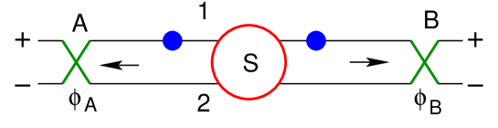
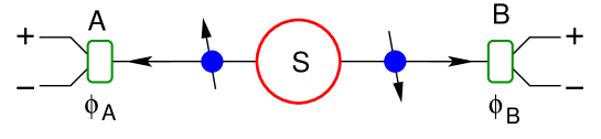
Figure 1: Picture of orbital (upper) and spin (lower) entanglement scheme. From the source S, an orbitally entangled, e.g. $|\tilde{\Psi}_{O}\rangle=1/\sqrt{2}(|1\rangle_{A}|1\rangle_{B}+|2\rangle_{A}|2\rangle_{B})$, or spin entangled, e.g. $|\tilde{\Psi}_{S}\rangle=1/\sqrt{2}(|\uparrow\rangle_{A}|\downarrow\rangle_{B}-|\downarrow\rangle_{A}|\uparrow\rangle_{B})$ state is emitted, with one particle propagating towards $A$ and one towards $B$. At $A$ and $B$, the particles are modulated, e.g. via single qubit rotations parameterized by angles $\phi_{A}$ and $\phi_{B}$. The particles are then detected in electronic reservoirs $+$ and $-$.

It is mainly the prospect of quantum information processing in solid state conductors that has motivated the recent interest in entanglement in mesoscopic conductors. In this work we do however not try to answer the ambitious question what quantum information tasks can be performed in mesoscopic systems. We do also not consider any particular measure of entanglement, instead we focus the discussion on the entangled quantum state. Given the state, the entanglement, quantified by ones measure of liking, can in principle be calculated. Therefore we are interested in the basic first step in a quantum information processing scheme, namely the creation, manipulation and detection of quasiparticle entanglement. A large number of implementations of this first step have been proposed, typically a certain mechanism is suggested that leads to emission of entangled particles from a ”source” S. The particles propagate out to spatially separated regions A and B, where they are manipulated and detected. Two schematics of generic systems for orbital and spin entanglement are shown in Fig. 1.

Very recently, in a number of works [1, 2, 3, 4, 5, 6, 7, 8, 9, 10, 11] entanglement in systems of quasiparticles has been investigated within the framework of scattering theory. These proposals are of particular interest because working with independent particles allows for a complete characterization of the emitted many-body state for arbitrary scattering amplitudes. Moreover, the notion of entanglement without direct interaction between the quasiparticles, a known concept in the theory of entanglement [25], has appeared puzzling to members of the mesoscopic community. The perception in the mesoscopic physics community has started to change only with the apperance of Ref. [2]. This makes it important to thoroughly analyze the origin of the entanglement. Here we contribute to such an analysis, focusing on the creation of entangled two-particle states due to redefinition of the vacuum. For comparison, an approach based on the reduced two-particle density matrix is discussed as well. Although not investigated here, it is probable that the two types of states turn out to be of different “usefulness” for quantum information processing, making a detailed comparision of interest. We start by stating some important general properties of entanglement and comment on their application to entanglement in mesoscopic conductors.

i) The entanglement of a state in a given system depends on how the system is formally parted in to subsystems [26]. If the system is considered as one entity, i.e. with all quasiparticles living in the same Hilbert space, one has to consider the question of entanglement of indistinguishable particles [27, 28]. For a mesoscopic system of independent fermionic quasiparticles, the ground state is given by a product state in occupation number formalism, i.e. the wavefunction is a single Slater determinant. Apart from the correlations due to fermionic statistics the particles show no correlations and the state is not entangled. However, if the system is considered as consisting of several spatially separated subsystems, one can pose questions about the entanglement between spatially separated, distinguishable quasiparticles living in the different subsystems. The latter is typically the case in the proposed mesoscopic systems (see Fig. 1), which are naturally parted into the source S and the two regions A and B. The entanglement between two particles, one in A and one in B, is in many situations nonzero. Quite generally, the physically relevant partitions into subsystems are defined by the system geometry and the possible measurements one can perform on the system [29, 30].

ii) The entanglement that can be investigated and quantified is determined by the possible measurements one can perform on the system. Although a wide variety of measurements in mesoscopic conductors in principle can be imagined, the most commonly measured quantities are currents and current correlators, i.e. current noise [31, 32]. In particular, in several recent works it was proposed to detect entanglement via measurements of current correlators [1, 2, 3, 5, 6, 7, 8, 9, 10, 11, 12, 33, 34]. This leads us to focus the discussion on entanglement detectable with current correlation measurements. All current cross correlation measurements, needed to investigate spatially separated particles, are to date measurements of second order correlators. Importantly, the second order current correlators are two-particle observables and can thus only provide direct information about two-particle entanglement. We thus limit our investigations here to the two-particle properties of the state [35].

Considering the typical mesoscopic entanglement setup in Fig. 1, the points i) and ii) lead us to discuss the entanglement between two spatially separated particles, one in A and one in B, detectable via correlations of currents flowing out into the reservoirs. Such a bipartite system is also the most commonly considered one in investigations of entanglement. Importantly, the entanglement can be both in the orbital [1] as well as in the spin degrees of freedom, the relevant entanglement depends on the proposed system geometry which can be designed to investigate orbital [1, 2, 3, 7] or spin [4, 5, 6, 10, 11, 12, 33, 47] entanglement. We also note that our measurement based scheme excludes all types of occupation number or Fock-space entanglement, e.g. the linear superposition of two particles at $A$ and two at $B$ [which in an occupation number notation can be written as the Fock-space entangled state $|0\rangle_{A}|2\rangle_{B}+|2\rangle_{A}|0\rangle_{A}$]. There is thus no need to enforce additional constraints [36, 37] on the state to exclude the physically irrelevant Fock-space entanglement.

3 System and scattering state.

To clearly illustrate the basic principles, we present here the formalism for independent quasiparticles in the most elementary mesoscopic system possible. We focus the discussion on the orbital entanglement which has the advantage that it can be manipulated and detected [1, 3] with existing experimental techniques. However, for completeness, spin information is retained throughout the discussion.

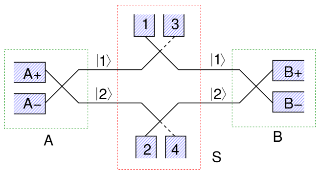
Figure 2: Schematic of the entanglement setup. The source region $S$ (dashed red box) consists of two beamsplitters connected to four reservoirs $1,2,3$ and $4$. The regions $A$ and $B$ (dashed blue boxes) consist of one beamsplitter and two reservoirs each. The orbital modes $|1\rangle$ and $|2\rangle$ out of the source region are displayed. Reservoirs $1$ and $2$ are kept at a potential $V$, the remaining reservoirs are grounded.

The system is shown in Fig. 2. In the source region, two single mode reflectionless beamsplitters are connected to four electronic reservoirs $1,2,3$ and $4$. A voltage bias $V$ is applied to reservoirs $1$ and $2$, while reservoirs $3$ and $4$ are kept at zero bias. Quasiparticles injected from reservoirs $1$ and $2$ scatter at the beamsplitters and propagate out towards regions $A$ and $B$. In $A$ and $B$, the quasiparticles are scattered at another pair of beamsplitters (i.e. a local single qubit rotation) and then detected in four reservoirs $A+,A-,B+$ and $B-$, all kept at zero potential. We emphasize that all components of this system can be realized in a conductor in the quantum Hall regime [3].

In this work we are interested in the entanglement of the state emerging from the source region, before the quasiparticles reach the beamsplitters in regions $A$ and $B$. The manipulation and detection processes taking place in $A$ and $B$ are thus not investigated. The two orbital modes $|1\rangle$ and $|2\rangle$, with labels $1$ and $2$ denoting from which reservoir the particles are emerging (see Fig. 2), constitute the orbital two-level, or pseudo-spin, system. Working within the quasiparticle scattering approach [32], we introduce operators $a_{m\sigma}^{\dagger}(E)$ creating electron quasiparticles at energy $E$ with spin $\sigma$, incident from reservoirs $m=1,2,3$ and $4$. The energy is counted from the Fermi level of the unbiased reservoirs. The transport state of the system at zero temperature is given by

$$|\Psi\rangle=\prod_{0<E<eV}a_{1\uparrow}^{\dagger}(E)a_{1\downarrow}^{\dagger}(E)a_{2\uparrow}^{\dagger}(E)a_{2\downarrow}^{\dagger}(E)|0\rangle$$ (1)

where $|0\rangle$ is the quasiparticle vacuum, a filled Fermi sea at energies $E<0$. This describes filled, noiseless streams of electrons emitted from reservoirs $1$ and $2$, propagating towards the first pair of beamsplitters. To describe the state after scattering at the beamsplitters, we introduce operators $b_{Am^{\prime}\sigma^{\prime}}(E)$ and $b_{Bm^{\prime}\sigma^{\prime}}(E)$ for particles originating from reservoir $m^{\prime}$, propagating from the beamsplitters towards regions $A$ and $B$ respectively. The operators $b_{Am^{\prime}\sigma^{\prime}}(E)$ and $b_{Bm^{\prime}\sigma^{\prime}}(E)$ are related to $a_{m\sigma}(E)$ via the scattering matrices of the beamsplitters. For simplicity we consider identical beamsplitters, taken independent on $E$ and $\sigma$, giving (suppressing spin and energy index)

$$\left(\begin{array}[]{c}b_{A1}\\ b_{B1}\end{array}\right)=\left(\begin{array}[]{cc}r&t^{\prime}\\ t&r^{\prime}\end{array}\right)\left(\begin{array}[]{c}a_{1}\\ a_{3}\end{array}\right),\hskip 2.84544pt\left(\begin{array}[]{c}b_{A2}\\ b_{B2}\end{array}\right)=\left(\begin{array}[]{cc}r&t^{\prime}\\ t&r^{\prime}\end{array}\right)\left(\begin{array}[]{c}a_{2}\\ a_{4}\end{array}\right)$$ (2)

We note that only static scatterers are considered here, the discussion could however straightforwardly be extended to time dependent scatterers, recently investigated in the context of entanglement in Refs. [38, 39].

To simplify the notation, a collective quantum number $n=\{1\uparrow,1\downarrow,2\uparrow,2\downarrow\}$ denoting both orbital mode and spin is introduced. The state describing particles propagating out towards $A$ and $B$ can then be written

$$|\Psi\rangle = \prod_{0<E<eV,n}\left[rb_{An}^{\dagger}(E)+tb_{Bn}^{\dagger}(E)\right]|0\rangle$$ (3)

Due to the scattering, the outflowing streams are noisy and the properties of the particles flowing towards $A$ and $B$ can be investigated via noise measurements. Here we are interested in the entanglement between two particles in the outflowing streams, one towards $A$ and one towards $B$. Importantly, the state $|\Psi\rangle$ in Eq. (3) is a many-body state, it describes a linear superposition of different number of particles at $A$ and $B$, ranging from zero to in principle infinity. Since only two-particle entanglement is considered, one thus needs to deduce the two-particle properties of the state $|\Psi\rangle$. Below we present two different approaches to do this, giving rise to two different quantum states with in general different entanglement.

4 Reduced two-particle density matrix approach.

We first discuss a general approach, applicable for arbitrary scattering amplitudes. Starting with the properties of the correlators of outflowing currents towards A and B, we note that the cross correlators (in the most general situation) are determined by averages of the type [32]

$$\langle b_{An}^{\dagger}(E)b_{Am}(E^{\prime})b_{Bk}^{\dagger}(E^{\prime\prime})b_{Bl}(E^{\prime\prime\prime})\rangle$$ (4)

$$= \langle b_{An}^{\dagger}(E)b_{Bk}^{\dagger}(E^{\prime\prime})b_{Bl}(E^{\prime\prime\prime})b_{Am}(E^{\prime})\rangle\propto\rho_{nm}^{kl}(E,E^{\prime},E^{\prime\prime},E^{\prime\prime\prime})$$

using in the second step the anticommutation relations for fermionic operators. The term $\rho_{nmkl}(E,E^{\prime},E^{\prime\prime},E^{\prime\prime\prime})$ is by definition an element of the reduced two-particle density matrix (in the energy basis). The current correlators are thus fully characterized by the reduced two-particle density matrix

$$\rho = \sum_{nmkl}\int dEdE^{\prime}dE^{\prime\prime}dE^{\prime\prime\prime}\rho_{nm}^{kl}(E,E^{\prime},E^{\prime\prime},E^{\prime\prime\prime})$$ (5)

$$\times b^{\dagger}_{An}(E)b_{Bk}^{\dagger}(E^{\prime\prime})|0\rangle\langle 0|b_{Bl}(E^{\prime\prime\prime})b_{Am}(E^{\prime}).$$

Accordingly, the entanglement potentially detectable via noise measurements is the entanglement of the reduced two-particle density matrix. Clearly, this is the situation for any two-particle observable. It should be emphasized that the two-particle density matrix physically describes the correlations of two particles out of the streams flowing towards $A$ and $B$, leaving all other particles unobserved. This is qualitatively different from a projection of a two-particle state out of the full many-body state, where only the components of the state containing exactly two particles are selected. It is shown below that these two different ways of extracting a two-particle state out of a many particle state can give rise to different states, and consequently to different entanglement.

Even with the object of interest confined to the reduced two-particle density matrix, a full characterization of the entanglement is cumbersome since $\rho$ is in general a mixed state and the two particles live in infinite dimensional Hilbert spaces spanned by $\{E,n\}$. In some simple situations (see e.g. below), the density matrix in Eq. (5) can be written as a direct product of the density matrices for the different degrees of freedom, e.g. $\rho=\rho_{O}\otimes\rho_{S}\otimes\rho_{E}$, where the subscripts $O,S$ and $E$ denote orbital, spin and energy respectively. This allows one to independently characterize the entanglement with respect to the different degrees of freedom. In particular, the orbital subspace in Fig. 2 and in e.g. Refs. [1, 2, 3] as well as generically the spin 1/2 space are two-level systems or qubits, giving rise to a system of two coupled qubits, well studied in the entanglement literature (see e.g. Ref. [40])

However, in the general case, with arbitrary scattering amplitudes, the reduced two-particle density matrix can not be written as a direct product, i.e. $\rho\neq\rho_{O}\otimes\rho_{S}\otimes\rho_{E}$. What can then be said about the entanglement? Of particular interest is the entanglement detectable via zero frequency current correlators, generally the quantity investigated in experiments. The zero frequency limit effectively projects the operators in Eq. (4) to the same energy [32] . For scattering amplitudes independent on energy on the scale of $eV$, the energy argument in Eq. (5) can be suppressed, giving a reduced density matrix

$$\bar{\rho} = \sum_{nm,kl}\rho_{nm}^{kl}b^{\dagger}_{An}b_{Bk}^{\dagger}|0\rangle\langle 0|b_{Bl}b_{Am},\hskip 14.22636pt\rho_{nm}^{kl}\propto\langle b_{An}^{\dagger}b_{Bk}^{\dagger}b_{Bl}b_{Am}\rangle.$$ (6)

The density matrix $\bar{\rho}$ contains information about the orbital and spin parts of the state only. Interestingly, following the opposite approach and considering the quasiparticle ($E>0$) correlator for coincident times, closely related to the electronic counterpart [3] to the joint detection probability introduced by Glauber [41] in quantum optics, one finds the same reduced density matrix $\bar{\rho}$ as in the zero frequency limit. Similar results for short time current correlators have been obtained in Refs. [5, 9, 10, 11].

The reduced density matrix $\bar{\rho}$ for the system under consideration (see Fig. 2) is evaluated from Eqs. (1), (2) and (6) to be

$$\bar{\rho}=\frac{1}{8}\left({\bf 1}_{O}\otimes{\bf 1}_{S}-F_{O}\otimes F_{S}\right),\hskip 14.22636ptF=\left(\begin{array}[]{cccc}1&0&0&0\\ 0&0&1&0\\ 0&1&0&0\\ 0&0&0&1\end{array}\right)$$ (11)

expressed in the orbital basis $\{|1\rangle_{A}|1\rangle_{B},|1\rangle_{A}|2\rangle_{B},|2\rangle_{A}|1\rangle_{B},|2\rangle_{A}|2\rangle_{B}\}$ and the spin basis $\{|\uparrow\rangle_{A}|\uparrow\rangle_{B},|\uparrow\rangle_{A}|\downarrow\rangle_{B},|\downarrow\rangle_{A}|\uparrow\rangle_{B},|\downarrow\rangle_{A}|\downarrow\rangle_{B}\}$. Here ${\bf 1}$ is the $4\times 4$ unit matrix. Note that since the particles in $A$ and $B$ are distinguishable there is no need for anti-symmetrization and we can use the notation e.g. $a_{A1\uparrow}^{\dagger}a_{B2\downarrow}^{\dagger}|0\rangle=|1\rangle_{A}|2\rangle_{B}\otimes|\uparrow\rangle_{A}|\downarrow\rangle_{B}$. Formally, the first term in Eq. (11) results from the direct pairing of the operators in the bracket in Eq. (5) and is given by the direct product of the single particle density matrices at $A$ and $B$. The second term results from the exchange pairing. Since the direct term by definition does not describe any nonlocal correlations (it is a separable state with respect to $A$ and $B$), it is the exchange correlations which are responsible for the entanglement. For the current correlators, it should be noted that the first term determines the product of the averaged currents, while the second term determines the irreducible current correlators, i.e. the correlators of the current fluctuations, the noise. We also note that $\bar{\rho}$ is independent on scattering amplitudes, a consequence of the assumption of identical, spin independent beamsplitters.

As is clear from Eq. (11), even though we consider a simple geometry with spin-independent scattering, the reduced density matrix $\bar{\rho}$ is not a direct product between orbital and spin part, i.e. $\bar{\rho}\neq\rho_{O}\otimes\rho_{S}$. Many observables are however not sensitive to the spin degree of freedom, as is the case for cross correlators between total currents $I=I_{\uparrow}+I_{\downarrow}$, typically the cross correlators investigated in mesoscopic conductors. The effective orbital density matrix accessible via current correlators is then obtained by tracing $\bar{\rho}$ over the spin degree of freedom, giving

$$\rho_{O}\equiv\mbox{tr}_{S}\left[\bar{\rho}\right]=\frac{1}{6}\left(2{\bf 1}-F\right)=\frac{1}{6}\left({\bf 1}+2|\Psi_{O}\rangle\langle\Psi_{O}|\right)$$ (12)

with $|\Psi_{O}\rangle=1/\sqrt{2}\left[|1\rangle_{A}|2\rangle_{B}-|2\rangle_{A}|1\rangle_{B}\right]$. This state, an example of a Werner state [42], can via suitable local transformations be written on a separable form [43, 44] with respect to $A$ and $B$ and is consequently not entangled. We note that the same holds for the reduced spin density matrix $\rho_{S}$, obtained by tracing over orbital degrees of freedom.

A different situation occurs if one considers a spin-polarized system, as was done e.g. in [2, 3]. In this case the density matrix is purely orbital, obtained from Eq. (6) by suppressing the spin notation. For the system in Fig. 2 we obtain

$$\rho_{O}=\frac{1}{2}\left({\bf 1}-F\right)=|\Psi_{O}\rangle\langle\Psi_{O}|,\hskip 14.22636pt$$ (13)

an orbital singlet, i.e. a maximally entangled state, again independent on scattering amplitudes. This result can be understood by considering the energy and spin independent incoming two-particle state $|\Psi\rangle=a_{1}^{\dagger}a_{2}^{\dagger}|0\rangle$, the version of the state in Eq. (1) appropriate under the stated assumptions. The corresponding outgoing state is

$$|\Psi\rangle=\left[r^{2}b_{A1}^{\dagger}b_{A2}^{\dagger}+t^{2}b_{B1}^{\dagger}b_{B2}^{\dagger}+rt\left(b_{A1}^{\dagger}b_{B2}^{\dagger}-b_{A2}^{\dagger}b_{B1}^{\dagger}\right)\right]|0\rangle$$ (14)

The first two terms describe two particles at A or two at B, while the last term describes one particles at A and one at B. As is clear from Eq. (6), only the last term, which is just $|\Psi_{O}\rangle$, contributes to $\rho_{O}$. Importantly, for the two-particle state in Eq. (14), the reduced density matrix approach gives the same result as projecting out the part of the state which contains one particle at $A$ and one at $B$. Both procedures are thus equivalent to a post-selection of entanglement, as originally discussed in quantum optics [45] (see e.g. Ref. [46] for a discussion for fermions). Various issues of projection and post-selection were recently discussed in a number of works on entanglement in mesoscopic conductors with arbitrary scattering amplitudes [3, 7, 10, 11] (for a related discussion, see also [6]).

It is interesting to note the clear difference between an orbital state obtained by tracing $\bar{\rho}$ over the spin degrees of freedom and the orbital state in a spin polarized system. The difference can be attributed to the fact that only spins of the same spieces are nonlocally correlated, i.e. contribute to the entanglement of the state. Detecting (without spin resolution) two particles, one at $A$ and one at $B$, the probability of obtaining two identical spins is only one half, reducing the entanglement of the state to zero.

5 Tunneling limit, vacuum redefinition.

A qualitatively different approach to the characterization of the emitted state can be taken in the limiting case of a tunneling system, as was done in Refs. [1, 2, 3].

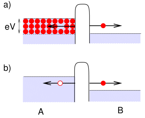
Figure 3: Pictures for particles flowing out from a beamsplitter in the source region. a) Single particle scattering picture. A transmission of a particle in the filled stream incident on the beamsplitter leads to creation of an electron flowing out towards $B$ and a missing electron, i.e. a hole, in the streams flowing out towards $A$. b) Electron-hole pair creation picture, the single particle scattering event creates an electron-hole pair on top of the redefined vacuum, with the electron moving out towards $B$ and the hole towards $A$.

Consider the state in Eq. (3). In the tunneling limit, $t\ll 1$, we can expand the product to first order in $t$ as

$$\prod_{0<E<eV,n}\left[rb_{An}^{\dagger}(E)+tb_{Bn}^{\dagger}(E)\right]$$

$$\hbox to0.0pt{\hss${}={}$}...\left[rb_{An}^{\dagger}(E)+tb_{Bn}^{\dagger}(E)\right]\left[rb_{An^{\prime}}^{\dagger}(E)+tb_{Bn^{\prime}}^{\dagger}(E)\right]...$$

$$\hbox to0.0pt{\hss${}\times{}$}\left[rb_{An}^{\dagger}(E^{\prime})+tb_{Bn}^{\dagger}(E^{\prime})\right]...\left[rb_{An}^{\dagger}(E^{\prime\prime})+tb_{Bn}^{\dagger}(E^{\prime\prime})\right]...$$

$$\hbox to0.0pt{\hss${}={}$}\prod_{0<E<eV,n}b_{An}^{\dagger}(E)+t\int_{0}^{eV}dE^{\prime}\sum_{n^{\prime}}..b_{An^{\prime}}^{\dagger}(E)..b_{Bn^{\prime}}^{\dagger}(E^{\prime})..b_{An}^{\dagger}(E^{\prime\prime})..$$ (15)

where the last term contains $b_{An}$ operators at all energies and $n$’s except $\{E^{\prime},n^{\prime}\}$, in the same order as in the line above (we consider a continuous spectrum). Using the property that $b_{An^{\prime}}(E^{\prime})b_{An^{\prime}}^{\dagger}(E^{\prime})|0\rangle=|0\rangle$ and that the operator products $b_{An^{\prime}}(E^{\prime})b_{An^{\prime}}^{\dagger}(E^{\prime})$ and $b_{Bn^{\prime}}(E^{\prime})^{\dagger}b_{An^{\prime}}(E^{\prime})$ commutes with all $b$-operators at different energies $E\neq E^{\prime}$ or $n\neq n^{\prime}$, we can write the state in Eq. (3) in a suggestive way by inserting $b_{An^{\prime}}(E^{\prime})b_{An^{\prime}}^{\dagger}(E^{\prime})$ in front of $|0\rangle$ and reordering the operators, giving

$$|\Psi\rangle = \prod_{0<E<eV,n}b_{An}^{\dagger}(E)|0\rangle$$ (16)

$$+ t\int_{0}^{eV}dE^{\prime}\sum_{n^{\prime}}b_{Bn^{\prime}}^{\dagger}(E^{\prime})b_{An^{\prime}}(E^{\prime})\prod_{0<E<eV}b_{An}^{\dagger}(E)|0\rangle$$

$$= \left[1+t\int_{0}^{eV}dE^{\prime}\sum_{n^{\prime}}b_{Bn^{\prime}}^{\dagger}(E^{\prime})b_{An^{\prime}}(E^{\prime})\right]\prod_{0<E<eV,n}b_{An}^{\dagger}(E)|0\rangle$$

The first term describes filled streams of quasiparticles flowing out towards $A$. The second term, with a small amplitude $t\ll 1$, describes the same filled streams with one electron missing and in addition a second electron propagating out towards $B$ (in mode $1$ or $2$). It is thus very natural to incorporate the filled, noiseless stream of quasiparticles flowing out towards $A$ into a new vacuum $|\bar{0}\rangle$, the second term then describes an electron-hole excitation out of the redefined vacuum. Formally, we can write the new vacuum in terms of the old vacuum $|0\rangle$ as

$$|\bar{0}\rangle=\prod_{0<E<eV,n}b_{An}^{\dagger}(E)|0\rangle$$ (17)

The new ground state is thus a filled Fermi sea at energies $E<0$ in $B$ and at $E<eV$ in $A$. The fermionic operators describing excitations out of the new vacuum are defined as

$$c^{\dagger}_{A\bar{n}}(E^{\prime})=\pm b_{An}(E),\hskip 14.22636ptc^{\dagger}_{Bn}(E)=b_{Bn}^{\dagger}(E)$$ (18)

where $\bar{n}$ denotes a spin opposite to $n$, $+(-)$ is for spin up (down) in $\bar{n}$ and $E^{\prime}=eV-E$. The transformation in Eq. (18) is thus equivalent to an inverse Bogoliubov transformation. We can then write the wavefunction in Eq. (16) as (reintroducing spin and orbital notation)

$$|\Psi\rangle=|\bar{0}\rangle+|\bar{\Psi}\rangle$$ (19)

with

$$|\bar{\Psi}\rangle=t\int_{0}^{eV}dE\sum_{j=1,2}\left[c_{B\downarrow j}^{\dagger}(E)c_{A\uparrow j}^{\dagger}(E^{\prime})-c_{B\uparrow j}^{\dagger}(E)c_{A\downarrow j}^{\dagger}(E^{\prime})\right]|\bar{0}\rangle$$ (20)

The wavefunction $|\bar{\Psi}\rangle$ describes a two-particle excitation, an electron-hole pair, out of the redefined vacuum $|\bar{0}\rangle$. The redefinition of the vacuum thus gives rise to a transformation from a picture with a many-body state of independent particles to a picture with two-particle excitations out of a ground state.

There are a number of important conclusions to be drawn from the result above, and to be put in relation to the result for the reduced density matrix approach:

(i) The state is wavepacket-like, i.e. it consists of a sum of electron-hole pairs at different energies, a detailed characterization of a similar wavepacket state emitted in a normal-superconductor system is given by us in Ref. [47]. As pointed out in Ref. [1], the average time between two subsequent wavepackets is much longer than the “width” of each wavepacket, i.e. subsequent entangled pairs are well separated in time, in contrast to the reduced two-particle state in the large transparency limit. This temporal separation probably makes the entangled state created by a redefinition of the vacuum more useful for quantum information processing, due to the possibility of addressing the individual entangled pairs. We remark that the formal procedure used above to calculate the state in Eq. (20) is essentially identical to the one for calculating the wavefunction of the two-photon state emitted in a parametric down conversion process in optics [48].

(ii) In a first quantization notation, we can write the wavefunction of the excitation

$$|\bar{\Psi}\rangle = t\int_{0}^{eV}dE\left[|1\rangle_{A}|1\rangle_{B}+|2\rangle_{A}|2\rangle_{B}\right]$$ (21)

$$\otimes \left[|\downarrow\rangle_{A}|\uparrow\rangle_{B}-|\uparrow\rangle_{A}|\downarrow\rangle_{B}\right]\otimes|E^{\prime}\rangle_{A}|E\rangle_{B}$$

This state is a direct product of the orbital, spin and energy parts of the state, in contrast to the general situation for the reduced two-particle state. Both the orbital and the spin state are maximally entangled Bell states. The spin state is a singlet as one would expect of an excitation out of a spinless groundstate, created by spin-independent scattering.

(iii) As was emphasized in Ref. [2], the redefinition of the vacuum is possible only in fermionic systems, i.e. it relies on the existence of a filled Fermi sea such that a removal of an electron below the Fermi energy creates a hole quasiparticle. This is further emphasized by the fact that the new groundstate, just as the initial one is noiseless.

(iv) The correlators between electron currents are simply related to the correlators between electron and hole currents as $\langle\Delta I^{e}(t)\Delta I^{h}(t^{\prime})\rangle=-\langle\Delta I^{e}(t^{\prime})\Delta I^{e}(t)\rangle$. Consequently, the electron-hole correlators are experimentally accessible and the electron-hole entanglement is, in line with the discussion above, a physically relevant object to study.

Importantly, the redefinition of the vacuum and the transformation to an electron-hole picture can be performed for an arbitrary transmission. However, in this case the resulting state describes a superposition of different numbers of electron-hole pairs. To obtain a two-particle state, one has to calculate a reduced electron-hole density matrix along the same line as in Eq. (5), i.e. replacing the electron operator $a_{An}^{\dagger}$ with the quasiparticle operator $c_{A\bar{n}}^{\dagger}$ etc. Performing such a calculation in the low transparency limit, one obtains as expected $|\bar{\Psi}\rangle\langle\bar{\Psi}|$, with $|\bar{\Psi}\rangle$ given by Eq. (21). It is however not possible from the reduced density matrix approach to conclude whether the emitted state is a true two-particle state or a reduced two-particle state.

For arbitrary scattering amplitudes, to quantitatively compare the reduced density matrix approach for electrons and holes to the results for electrons discussed above, we consider the simplest situation with low frequency correlators, i.e. all $c$-operators at equal energy, and a spin polarized conductor. The reduced orbital density matrix for the system in Fig. 2 is then given by

$$\rho_{O}^{eh}=\frac{1}{2(1+T)}\left[T{\bf 1}+2R|\tilde{\Psi}_{O}\rangle\langle\tilde{\Psi}_{O}|\right],$$ (22)

with $|\tilde{\Psi}_{O}\rangle=1/\sqrt{2}\left[|1\rangle_{A}|1\rangle_{B}+|2\rangle_{A}|2\rangle_{B}\right]$ and the scattering probabilities $R=1-T=|r|^{2}$. Interestingly, in contrast to the density matrix in Eq. (11), the density matrix $\rho_{O}^{eh}$ depends on the scattering probabilities. The state $\rho_{O}^{eh}$ is a Werner state, entangled for $R>T$. In the limit $T\ll 1$, one has $\rho_{O}^{eh}=|\tilde{\Psi}_{O}\rangle\langle\tilde{\Psi}_{O}|$, an orbital Bell state, maximally entangled. Moreover, away from the tunneling limit, the two-particle entanglement in the electron-hole picture is smaller than the entanglement in the electron picture [the state in Eq. (13) is maximally entangled]. This is in agreement with the findings of Lebedev et al [10], who investigated the conditions for a violation of a Bell Inequality for a scatterer with arbitrary transparency, comparing the electron and the electron-hole approaches.

The state $\rho_{O}^{eh}$ can be understood by considering the state in Eq. (14) after redefining the vacuum and transforming to an electron-hole picture, giving

$$|\Psi\rangle=\left[r^{2}+t^{2}c_{B1}^{\dagger}c_{B2}^{\dagger}c_{A1}^{\dagger}c_{A2}^{\dagger}+rt\left(c_{A1}^{\dagger}c_{B1}^{\dagger}+c_{A2}^{\dagger}c_{B2}^{\dagger}\right)\right]|\bar{0}\rangle$$ (23)

The last term is just $|\tilde{\Psi}_{O}\rangle$ while the second term, describing four particles, i.e. two electron-hole pairs, also contributes to the reduced density matrix in Eq. (22), it gives rise to the term $T{\bf 1}$. Interestingly, performing a projection of $|\Psi\rangle$ onto a state with only two particles, one in $A$ and one in $B$, one obtains the maximally entangled state $|\tilde{\Psi}_{O}\rangle$, since the terms with two electron-hole pairs are discarded. The projection approach thus, in the large transparency limit, overestimates the entanglement detectable via current correlations.

To illustrate the relevance of the vacuum redefinition, we now discuss two different systems where this was investigated.

6 Normal-Superconducting entangler.

We first consider the case of a normal-superconducting system, to large extent following Ref. [1]. As in all existing works on entanglement in normal-superconducting systems [4, 5, 47, 49, 51, 52, 53, 54, 55], we consider the superconductor in the mean-field description. The mean field Hamiltonian is bilinear in fermionic operators and is diagonalized by a Bogoliubov transformation, giving rise to a new set of independent electron and hole like quasiparticles. Importantly, although the microscopic mechanism for superconductivity is interaction between electron quasiparticles, in the mean field description it is again possible to find a picture with noninteracting quasiparticles. For a noninteracting normal conductor connected to a superconductor, the whole system can thus be treated within a single particle scattering approach to the Bogoliubov-de Gennes equation [56]. Consequently, the approach above to the entanglement for systems of independent quasiparticles can be applied.

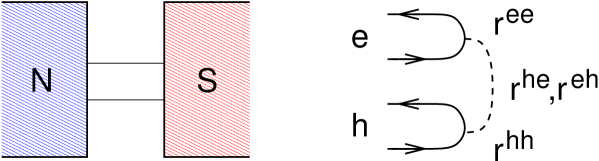
Figure 4: Schematic of the conductor. Left: Mesoscopic conductor contacted to a normal reservoir (blue shaded) and a superconducting reservoir (red shaded). Right: Paths of scattering particles at energies well below the superconducting gap. An incoming electron from the normal reservoir has the amplitude $r^{ee}$ to be reflected as an electron and $r^{he}$ to be reflected as a hole. For incoming holes, the corresponding amplitudes are $r^{eh}$ and $r^{hh}$.

To illustrate the basic principle of two-particle emission, we first consider the case of a two-mode (to connect to the orbital discussion above) normal-superconductor system shown in Fig. 4. At the normal-superconductor interface, for energies well below the superconducting gap, scattering occurs either as Andreev reflection or as normal reflection. Consider the situation with a negative bias $-eV$ applied at the normal reservoir while the superconducting reservoir is kept at zero potential. Counting the energy from the superconducting chemical potential $\mu_{S}$, we consider operators $a_{en}^{\dagger}(E)$ and $a_{hn}^{\dagger}(E)$, creating electron and hole quasiparticle excitations respectively at energy $E$ incident from the normal reservoir. The collective quantum number $n$ denotes as above orbital mode and spin. The state of the system at zero temperature is given by

$$|\Psi\rangle_{NS}=\prod_{0<E<eV,n}a^{\dagger}_{hn}(E)|0\rangle$$ (24)

describing a filled stream of holes injected from the normal reservoir, where $|0\rangle$ is the quasiparticle vacuum. The operators $a_{en}(E)$ and $a_{hn}(E)$ are related to operators $b_{en}(E)$ and $b_{hn}(E)$ for quasiparticles propagating back from the normal-superconducting interface towards the normal reservoir via the scattering matrix (again taken independent on $E$ and $n$) as

$$\left(\begin{array}[]{c}b_{e}\\ b_{h}\end{array}\right)=\left(\begin{array}[]{cc}r^{ee}&r^{eh}\\ r^{he}&r^{hh}\end{array}\right)\left(\begin{array}[]{c}a_{e}\\ a_{h}\end{array}\right)$$ (25)

The state $|\Psi\rangle_{NS}$ can then be written in terms of the $b$-operators

$$|\Psi\rangle_{NS} = \prod_{0<E<eV,n}\left[r^{eh}b_{en}^{\dagger}(E)+r^{hh}b_{hn}^{\dagger}(E)\right]|0\rangle$$ (26)

Considering the tunneling limit, the Andreev reflection amplitude $r^{eh}\ll 1$ and one can proceed in exactly the same way as in Eqs. (15) and (16) to arrive at the wavefunction to leading order in $r^{eh}$ as

$$|\Psi\rangle_{NS} = \left[1+r^{eh}\int_{0}^{eV}dE^{\prime}\sum_{n^{\prime}}b_{en^{\prime}}^{\dagger}(E^{\prime})b_{hn^{\prime}}(E^{\prime})\right]\prod_{0<E<eV,n}b_{hn}^{\dagger}(E)|0\rangle$$

The first term describes a filled stream of hole quasiparticles flowing back towards the normal reservoir. The second term, with a small amplitude $r^{eh}\ll 1$, describes the same filled stream with one hole missing and in addition a second electron propagating back. We can thus proceed as above and incorporate the filled, noiseless stream of hole quasiparticles flowing out towards the normal conductor into a new, redefined vacuum $|\bar{0}\rangle$, given by

$$|\bar{0}\rangle=\prod_{0<E<eV,n}b_{An}^{\dagger}(E)|0\rangle$$ (28)

The fermionic operators describing excitations of the new ground state are given by the Bogoliubow transformation

$$c^{\dagger}_{n}(E)=b_{en}^{\dagger}(E),\hskip 14.22636ptc^{\dagger}_{\bar{n}}(-E)=\pm b_{hn}(E)$$ (29)

where $\bar{n}$ denotes the spin-flip in the electron-hole transformation with $+(-)$ for spin up (down) in $\bar{n}$. Note that the $c$-operators are just standard electron operators. A missing hole in the filled hole stream is thus just an electron with opposite spin and energy compared to the superconducting chemical potential $\mu_{S}$.

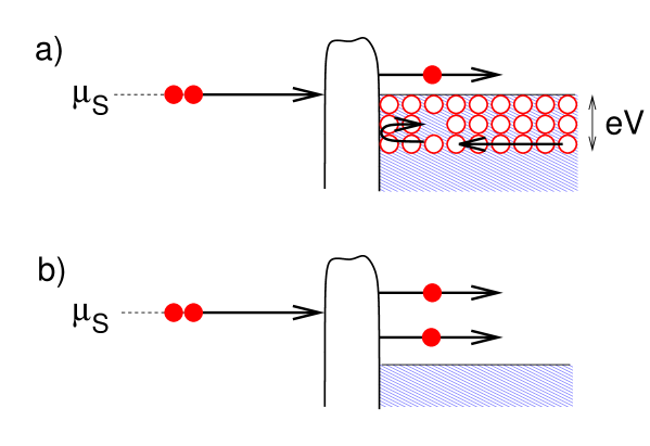
Figure 5: Schematic of a normal-superconducting interface. a) Bogoliubov-de Gennes picture, a filled stream of holes are incident on S from N. An Andreev reflection leads to creation of an electron above the superconducting chemical potential $\mu_{S}$ and a missing hole in the back-flowing hole stream. b) Cooper pair tunneling picture, a Cooper pair tunnels from S to N, leading to a pair of electrons in N, on top of the ground state.

We can then write the wavefunction in Eq. (16) as, reintroducing spin and orbital notation

$$|\Psi\rangle_{NS}=|\bar{0}\rangle_{NS}+|\bar{\Psi}\rangle$$ (30)

with

$$|\bar{\Psi}\rangle=r^{eh}\int_{0}^{eV}dE\sum_{j=1,2}\left[c_{j\uparrow}^{\dagger}(E)c_{j\downarrow}^{\dagger}(-E)-c_{j\downarrow}^{\dagger}(E)c_{j\uparrow}^{\dagger}(-E)\right]|\bar{0}\rangle$$ (31)

The wavefunction $|\bar{\Psi}\rangle$ thus describes a two-particle excitation, an electron pair or Cooper pair, out of the redefined vacuum $|\bar{0}\rangle$. The redefinition of the vacuum thus gives rise to a transformation from a picture with a many-body state of independent particles to a picture with two-electron excitations out of a ground state. We point out that this approach, shown schematically in Fig. 5, provides a formal connection between the scattering and the tunnel Hamiltonian approach (see e.g. Refs. [47, 49]).

To connect this two-particle emission to orbital entanglement, we consider as a concrete example our proposal in Ref. [1]. The system geometry is shown in Fig. 6, a multiterminal normal conductor connected via tunnel barriers to a single superconductor and further to four normal reservoirs. The two regions at $A$ and $B$, with an electronic beamsplitter and two reservoirs respectively, constitute the two subsystems. For details of the proposals we refer the reader to Ref. [1] and Ref. [57]. To first order in tunnel barrier transparency a pair of electrons is emitted on top of the new ground state, at interface $1$ or $2$.

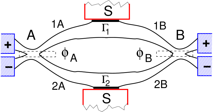
Figure 6: Orbital normal-superconductor entangler: A single superconductor (S) is connected to four normal arms via two tunnel barriers $1$ and $2$ (thick black lines). The arms are joined pairwise in beam splitters A and B and end in normal reservoirs labeled $+$ and $-$. After Ref. [1].

This leads to a state describing a linear superposition of pairs at $1$ and at $2$. Taking into account that the electrons can be emitted either towards $A$ or towards $B$, we have the emitted state given by $|\bar{\Psi}\rangle_{NS}=|\Psi_{1}\rangle_{NS}+|\Psi_{2}\rangle_{NS}$, where

$$|\tilde{\Psi}_{1}\rangle_{NS} = r^{eh}\int_{0}^{eV}dE\sum_{j=1,2}\sum_{\eta=A,B}\left[c_{\eta j\uparrow}^{\dagger}(E)c_{\eta j\downarrow}^{\dagger}(-E)\right.$$

$$\hskip 14.22636pt-\left.c_{\eta j\downarrow}^{\dagger}(E)c_{\eta j\uparrow}^{\dagger}(-E)\right]|\bar{0}\rangle,$$

$$|\tilde{\Psi}_{2}\rangle_{NS} = r^{eh}\int_{-eV}^{eV}dE\left[c_{A1\uparrow}^{\dagger}(E)c_{B1\downarrow}^{\dagger}(-E)-c_{A1\downarrow}^{\dagger}(E)c_{B1\uparrow}^{\dagger}(-E)\right.$$ (32)

$$+\left.c_{A2\uparrow}^{\dagger}(E)c_{B2\downarrow}^{\dagger}(-E)-c_{A2\downarrow}^{\dagger}(E)c_{B2\uparrow}^{\dagger}(-E)\right]|\bar{0}\rangle,$$

The state $|\tilde{\Psi}_{1}\rangle_{NS}$ describes a superposition of two particles at $A$ and two at $B$. This state does however not contribute to the noise correlators or, as is clearly the case, to the two-particle density matrix describing one particle at A and one at B. The state $|\tilde{\Psi}_{2}\rangle_{NS}$ however describes orbitally (as well as spin-entangled) electron “wave packet” pairs, with one particle at A and one at B. This is the entangled state detected by the noise.

7 Normal state entangler.

We then turn to a normal state entangler working in the Quantum Hall regime. Such a system was introduced by Beenakker et al in Ref. [2] and then later considered in [7]. In both Refs. [2] and [7], two parallel edgestates connected via a nonadiabatic, edge channel mixing scattering region was considered. In Ref. [3] we instead considered a topologically different Quantum Hall system, a Hanbury Brown Twiss geometry (or Corbino geometry) with only single edge-states and quantum point contacts. This highly simplifies the experimental realization of the proposal. The system is just a proposal for a physical realization of the system shown in Fig. 2, discussed in detail above, and we therefore keep the discussion short.

The system is shown in Fig. 7, for details we refer the reader to Ref. [3]. A spin-polarized edge state is considered. We take the transmission and reflection probabilities at the point contact $C$ to be $T_{C}=1-R_{C}=T$ and at $D$ to be $T_{D}=1-R_{D}=R$. After scattering at $C$ and $D$, the state $|\Psi\rangle$ consists of two contributions in which the two particles fly off one to $A$ and one to $B$, and of two contributions in which the two particles fly both off towards the same detector QPC.

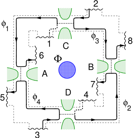
Figure 7: Normal-state orbital entangler: a rectangular Hall bar with inner and outer edges (thin dashed lines) and four quantum point contacts (grey shaded) with transparencies $T_{A},T_{B},T_{C}$ and $T_{D}$. Contacts $2$ and $3$ are sources of electrons (a voltage $eV$ is applied against all other contacts which are at ground). Electrons follow edge states (thick black lines) in the direction indicated by the arrows. An Aharanov-Bohm flux $\Phi$ penetrates the center of the sample (shaded). After Ref. [3].

Consider now the case of strong asymmetry $R\ll 1$, where almost no electrons are passing through the source QPC’s towards $B$. Performing the reformulation of the ground state and the transformation ta an electron-hole picture, we can directly write the full state $|\Psi\rangle$ to leading order in $\sqrt{R}$ as $|\Psi\rangle=|\bar{0}\rangle+\sqrt{R}|\tilde{\Psi}\rangle$, with

$$|\tilde{\Psi}\rangle=\int_{0}^{eV}dE\left[c_{3B}^{\dagger}(E)c_{3A}^{\dagger}(E)-c_{2B}^{\dagger}(E)c_{2A}^{\dagger}(E)\right]|\bar{0}\rangle$$ (33)

Due to the redefinition of the vacuum, we can interpret the resulting state $|\tilde{\Psi}\rangle$ as describing a superposition of ”wavepacket”-like electron-hole pair excitations out of the new vacuum, i.e. an orbitally entangled pair of electron-hole excitations. This is just equivalent to the result in Eq. (21).

8 Conclusions

We have presented a scattering approach to entanglement in mesoscopic conductors with independent fermionic quasiparticles. The role of the system geometry and accessible measurements in defining the relevant entanglement was discussed. As a simple example, a multiterminal mesoscopic conductor with spin-independent scattering was investigated in detail, deriving an expression for the manybody scattering state emitted by the conductor. The focus was on orbital entanglement, accessible with present day experimental technics.

Two different approaches to a two-particle state were considered. The main focus was on conductors in the tunneling limit, where entangled two-particle states arise from a redefinition of the quasiparticle vacuum. The redefinition of the vacuum leads to a transition from a picture with a many-body state of independent particles to a picture with two-particle excitations out of a new ground state. This was compared to the entanglement of an effective two-particle state, obtained by a reduced density matrix approach, applicable for conductors with arbitrary scattering amplitudes. Moreover, the qualitative difference between the reduced two-particle density matrix approach and a projection scheme was discussed.

We showed that the two different approaches, redefinition of the vacuum state and two-particle state reduction, in general give rise to different two-particle states and consequently to different entanglement. This was illustrated by investigating in detail the orbital entanglement for the simple mesoscopic conductor, focusing on the spin-polarized regime. In the tunneling limit, we applied our approach with the redefinition of the vacuum state to the systems proposed in Refs. [1], a normal-superconducting heterostructure, and in [3], a conductor in the Quantum Hall regime. This showed the qualitative as well as quantitative similarities between the entangled states emitted in the two systems.

References

References

- [1] P. Samuelsson, E.V. Sukhorukov, and M. Büttiker, Phys. Rev. Lett. 91, 157002 (2003).
- [2] C.W.J. Beenakker, C. Emary, M. Kindermann, J.L. van Velsen, Phys. Rev. Lett. 91, 147901 (2003).
- [3] P. Samuelsson, E.V. Sukhorukov, and M. Büttiker, Phys. Rev. Lett. 92, 026805 (2004).
- [4] G.B. Lesovik, T. Martin and G. Blatter, Eur. Phys. J. B 24, 287 (2001).
- [5] N. M. Chtchelkatchev, G. Blatter, G. B. Lesovik, Th. Martin, Phys. Rev. B 66, 161320 (2002).
- [6] L. Faoro, F. Taddei, and R. Fazio, Phys. Rev. B 69, 125326 (2004).
- [7] C.W.J. Beenakker, M. Kindermann, Phys. Rev. Lett. 92, 056801 (2004).
- [8] M. Büttiker, P. Samuelsson and E.V. Sukhorukov, Physica E 20, 33 (2003).
- [9] C.W.J. Beenakker, M. Kindermann, C.M. Marcus, A. Yacoby, Fundamental Problems of Mesoscopic Physics, eds. I.V. Lerner, B.L. Altshuler, and Y. Gefen, NATO Science Series II. Vol. 154 (Kluwer, Dordrecht, 2004).
- [10] A. V. Lebedev, G. B. Lesovik, G. Blatter, Phys. Rev. B 71, 045306 (2005).
- [11] A. V. Lebedev, G. Blatter, C. W. J. Beenakker, G. B. Lesovik, Phys. Rev. B 69, 235312 (2004).
- [12] A. Di Lorenzo, Yu. V. Nazarov, cond-mat/0408377.
- [13] E. Schrödinger, Naturwissenschaften, 23, 807 (1935); 23, 844 (1935).
- [14] A. Einstein, B. Podolsky and N. Rosen, Phys. Rev. 47, 777 (1935).
- [15] J.S. Bell, Physics 1, 195 (1965); Rev. Mod. Phys. 38, 447 (1966).
- [16] W. Tittel, J. Brendel, H. Zbinden, and N. Gisin, Phys. Rev. Lett 81, 3563 (1998).
- [17] G. Weihs, T. Jennewein, C. Simon, H. Weinfurter and A. Zeilinger, Phys. Rev. Lett 81, 5039 (1998).
- [18] A. Aspect, Nature 398, 189 (1999).
- [19] M. Nielsen and I. Chuang, Quantum Computation and Quantum Information (Cambridge Univ. Press, Cambridge, 2000).
- [20] A.K. Ekert, Phys. Rev. Lett. 67, 661 (1991).
- [21] C.H. Bennett, G. Brassard, C. Crépeau, R. Josza, A. Peres, and W.K. Wooters, Phys. Rev. Lett. 70, 1895 (1993).
- [22] C.H. Bennett and S.J. Wiesner, Phys. Rev. Lett. 69, 2881 (1992).
- [23] M. Keyl, Phys. Rep. 369, 431 (2002).
- [24] D. Bruss, J. Math. Phys, 43, 4237 (2002).
- [25] For some recent illuminating examples, see e.g. V. Vedral, quant-ph/0302040.
- [26] A. Peres, Quantum theory: concepts and methods, Doordrecht, Kluwer, 1993.
- [27] J. Schliemann, D. Loss, and A. H. MacDonald, Phys. Rev. B 63, 085311 (2002).
- [28] K. Eckert, J. Schliemann, D. Bruss, and M. Lewenstein, Ann. Phys. 299, 88 (2002).
- [29] P. Zanardi, Phys. Rev. Lett. 87, 077901 (2001).
- [30] P. Zanardi, D. Lidar, and S. Lloyd, Phys. Rev. Lett. 92, 060402 (2004).
- [31] M. Büttiker, Phys. Rev. B 46, 12485 (1992).
- [32] Ya. M. Blanter and M. Büttiker, Phys. Rep. 336, 1 (2000).
- [33] G. Burkhard, D. Loss, and E.V. Sukhorukov, Phys. Rev. B 89, 176401 (2000).
- [34] X. Maitre, W.D. Oliver, and Y. Yamamoto, Physica E 6, 301 (2000).
- [35] For works on multiparticle entanglement in mesoscopic systems and detection schemes based on higher order current correlators, see C.W.J. Beenakker, M. Kindermann, Phys. Rev. Lett. 92, 056801 (2004) and C.W.J. Beenakker, C. Emary, M. Kindermann, Phys. Rev. B 69, 115320 (2004).
- [36] S. D. Bartlett, H. M. Wiseman, Phys. Rev. Lett. 91, 097903 (2003).
- [37] H. M. Wiseman, S. D. Bartlett, J. A. Vaccaro, quant-ph/0309046.
- [38] P. Samuelsson and M. Büttiker, cond-mat/0410581.
- [39] C.W.J. Beenakker, M. Titov, B. Trauzettel, cond-mat/0502055.
- [40] W. Wooters, Phys. Rev. Lett 80, 2245 (1998).
- [41] R. Glauber, Phys. Rev. 130, 2529 (1963).
- [42] R.F. Werner, Phys. Rev. A 40, 4277 (1989).
- [43] A. Peres, Phys. Rev. Lett 77, 1413 (1996).
- [44] M. Horodecki, P. Horodecki, and R. Horodecki, Phys. Lett. A 223, 1 (1996).
- [45] Y.H. Shih and C.O. Alley, Phys. Rev. Lett. 61, 2921 (1988).
- [46] S. Bose and D. Home, Phys. Rev. Lett. 88, 050401 (2002).
- [47] P. Samuelsson, E.V. Sukhorukov, and M. Büttiker, Phys. Rev. B 70, 115330 (2004).
- [48] Z. Y. Ou, L. J. Wang, X. Y. Zou, and L. Mandel, Phys. Rev. A 41, 566 (1990).
- [49] P. Recher, E. V. Sukhorukov, and D. Loss, Phys. Rev. B 63, 165314 (2001).
- [50] E. Prada and F. Sols, Eur. Phys. J. B 40, 379 (2004).
- [51] P. Recher and D. Loss, Phys. Rev. B 65, 165327 (2002).
- [52] C. Bena, S. Vishveshwara, L. Balents and M. P. A. Fisher, Phys. Rev. Lett 89, 037901 (2002).
- [53] P. Recher and D. Loss, Phys. Rev. Lett 91, 267003 (2003).
- [54] V. Bouchiat, N. Chtchelkatchev, D.Feinberg, G.B. Lesovik, T. Martin, J. Torres, Nanotechnology 14, 77 (2003).
- [55] O. Sauret, T. Martin, D. Feinberg, cond-mat/0410325.
- [56] S. Datta, P.F. Bagwell and M.P. Anantram, Phys. Low-Dim. Struct. 3, 1 (1996).
- [57] P. Samuelsson, E. V. Sukhorukov and M. Büttiker, Turk. J. Phys. 27, 481 (2003).