Exact Solution of a Field Theory Model of Frontal Photopolymerization

Abstract

Frontal photopolymerization (FPP) provides a versatile method for the rapid fabrication of solid polymer network materials by exposing photosensitive molecules to light. Dimensional control of structures created by this process is crucial in applications ranging from microfluidics and coatings to dentistry, and the availability of a predictive mathematical model of FPP is needed to achieve this control. Previous work has relied on numerical solutions of the governing kinetic equations in validating the model against experiments because of the intractability of the governing non-linear equations. The present paper provides exact solutions to these equations in the general case in which the optical attenuation decreases (photobleaching) or increases (photodarkening) with photopolymerization. These exact solutions are of mathematical and physical interest because they support traveling waves of polymerization that propagate logarithmically or linearly in time, depending on the evolution of optical attenuation of the photopolymerized material.

I Introduction

Photopolymerization is a common method of rapidly forming solid network polymer materials and it is possible to create intricate three-dimensional structures by selectively polymerizing photosensitive materials through masks opaque to light. The conversion process from a liquid to a solid does not occur uniformly in this fabrication technique because of the attenuation of light within the photopolymerizable material (PM) and this process is normally accompanied by non-uniform monomer-to-polymer conversion profiles perpendicular to the illuminated surface Odian (1991); Fouassier (1995); Fouassier and Rabek (1993); Decker (1998, 2002). Physically, these conversion profiles propagate as traveling waves of network solidification that invade the unpolymerized medium exposed to radiation (generally ultraviolet light, UV) if the process occurs in the presence of strong optical attenuation and limited mass and heat transfer. The frontal aspect of the polymerization process is apparent in the photopolymerization of thick material sections and has counterparts in degradation (including discoloration) processes in polymer films exposed to UV radiation, where the breaking of chemical bonds rather than their formationis often the prevalent physical process.

Frontal photopolymerization (FPP) is utilized in diverse fabrication processes, ranging from photolithography of microcircuits to dental restorative and other biomedical materials, and numerous coatings applications (paints and varnishes, adhesives and printing inks) Decker (1998, 2002). We have recently explored the use of FPP in the fabrication of microfluidic devices Harrison et al. (2004); Cabral et al. (2004); Wu et al. (2004); Cygan et al. (2005); Hudson et al. (2004).

We emphasize that FPP is a distinct mode of polymerization from thermal (TFP) and isothermal (IFP) frontal polymerization, which involve autocatalytic reactions. While these polymerization methods also involve wavelike polymerization fronts, the front propagation is sustained by the thermal energy released from an exothermic polymerization reaction. This self-propagating frontal growth can be initiated by a localized heat source (TFP) of by a polymer network seed (IFP) and has been reviewed by Pojman et al. Khan and Pojman (1996); Pojman et al. (1996); Lewis et al. (2004).

Given the complexity of the chemical reactions involved in FPP, a ‘minimal’ field theoretic model of this process was introduced in previous work based on physical observables relevant to the fabrication process Cabral et al. (2004); Cabral and Douglas (2005). Specifically, this FPP model concerns itself with two basic front properties and their evolution in space and time: (1) the position of the solid/liquid front, which defines the patterned height and (2) the light transmission of the PM layer. This formulation naturally leads to a system of coupled partial differential equations involving two coupled field variables, the extent of monomer-to-polymer conversion $\phi(x,t)$ and the light attenuation $Tr(x,t)$ as a function of the distance from the illuminated surface $x$ and time $t$.

Before describing our mathematical model, we briefly illustrate the physical nature of FPP through experiments on a model UV polymerizable material, described in Section II and discussed in Section III. The derivation of this model is reviewed in Section IV and Section V presents exact solutions of these non-linear equations.

II Experimental

The photopolymerization experimental setup dis consists of a collimated light source, a photomask, a polymer photoresist and a substrate, as depicted in Fig. 1. We choose a multifunctional thiol-ene formulation (NOA81, Norland Products, NJ) as the photopolymerizable material (PM) for this study. This optically clear, liquid PM functions as a negative photoresist and cures under 365 nm ultraviolet light (UVA) into a hard solid (Shore D durometer 90 and $\sim$ 1 GPa modulus). Moreover, thiol-enes polymerize rapidly at ambient conditions (with minimal oxygen inhibition) and achieve large depths of cure Jacobine (1993); Cramer et al. (2002, 2003); Reddy et al. (2003). In previous work, we have characterized the kinetics of FPP of these systems as a function of PM composition, temperature and nanoparticle loading Cabral et al. (2004); Cabral and Douglas (2005).

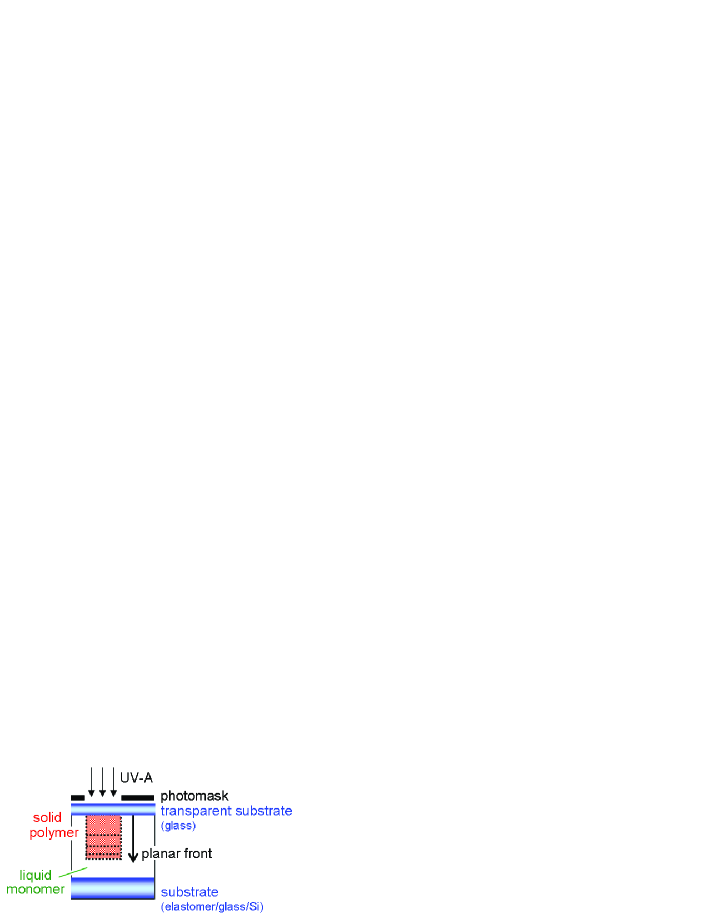
Figure 1: Schematic of the frontal photopolymerization (FPP), depicting a monomer-to-polymer conversion front induced by light exposure moving towards the bulk polymerizable material (PM). Our experimental setup consists of a collimated UV source (365 nm), a photomask, and a PM confined between two surfaces, typically glass and an elastomer sheet.

The liquid PM was poured into an elastomeric (polydimethylsiloxane, Sylgard 184, Dow Corning) gasket and covered with a plasma-cleaned glass slide (Corning 2947). The oxygen plasma was an Anatech-SP100 operating at 80 Pa (600 mTorr), with 60 W for 3 min. Photomasks were printed on regular acetate sheet transparencies (CG3300, 3M) using a 1200 dots per inch HP Laserjet 8000N printer. The mask consisted of a square array of large posts (2 mm $\times$ 2 mm) and was placed directly over the top glass slide. An aluminum shutter was placed over the specimen and moved manually, controlling the exposure time of each post. The light source was a Spectroline SB-100P flood lamp, equipped with a 100 Watt Mercury lamp (Spectronics), placed at a variable distance (100’s of mm) from the specimen to adjust the incident intensity. The light intensity was measured with a Spectroline DIX-365A UV-A sensor and DRC-100X radiometer (both Spectronics) with 0.1 $\mu$W/mm² (10 $\mu$W/cm²) resolution. The UV dose administered to each patterned post was calculated as the product of the incident light intensity $I_{0}\equiv I(x=0)$, light transmission $Tr$ of the mask ($\sim$ 80 %) and glass slide ($\sim$ 94 %), and exposure time $t$, as $UVdose\equiv TrI_{0}t$ ; $x$ is depth distance normal to the surface in the PM. Photopolymerization was carried out under a fume hood at 30 ^∘C, with incident light intensity of (2 and 10) $\mu$W/mm²; a wide UV dose window covering 0.04 mJ/mm² to 180 mJ/mm² was investigated.

Upon UV light exposure, imaged areas become insoluble to selective solvents ethanol and acetone, which are used to develop the pattern. Compressed air and a succession of alternating ethanol/acetone rinses are employed until the unpolymerized material is thoroughly removed. The resulting pattern has well defined dimensions but is still a ‘soft’ solid. A flood UV exposure (for about 50 times the patterning dose), completes the crosslinking process of the material into a hard solid, largely preserving its dimensions. The topography of the resulting photopolymerized structure was mapped by stylus profilometry, using a Dektak 8 profilometer (Veeco, CA), equipped with a 12.5 $\mu$m stylus and operating at 10 mg force. For post heights beyond the profilometer 1 mm limit, a caliper (Digit-cal MK IV, Brown & Sharpe) was utilized. Measurement uncertainty ranged from 5 % to 10 %, depending on the pattern height. A typical profilometer scan of two arrays of posts exposed to increasing UV doses is shown in Fig. 2. The resulting patterned dimensions range from approximately 70 to 1000 $\mu$m in height.

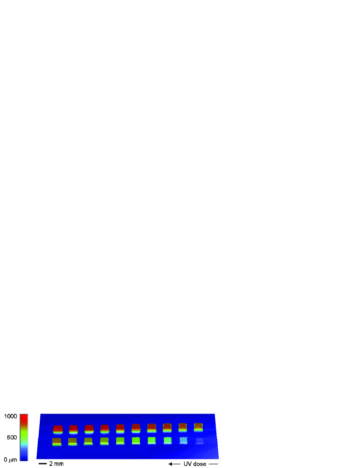
Figure 2: Topography map of an array of FPP squares obtained by stylus profilometry. The exposure time for each square was defined by a shutter system and was varied linearly in 30 s intervals, totaling 10 min. The resulting heights $h(t)$, however, increase in a strongly non-linear fashion, apparently leveling off at long exposures. The incident intensity was 1.8 $\mu$W/mm² and the UV dose window sampled was (0.05 to 10) mJ/mm².

In order to explore the spatio-temporal variation of the light intensity upon photocuring, a second series of experiments were devised. The transmission of PM samples of different thickness was monitored as a function of time during the conversion process. The PM was confined between transparent glass slides with spacers of defined thickness; this assembly was placed between the UV source and the radiometer and the transmitted light intensity was recorded as a function of time. Sample thickness was limited to 1 mm due to light attenuation and sensor sensitivity to the actinic wavelength. The effective sample transmission $Tr(x,t)$ was obtained from the recorded intensity $I(x,t)$ and the Beer-Lambert relation $Tr(x,t)\equiv(I(x,t)/I_{0})/Tr(glass)^{2}=\exp\left[-\bar{\mu}(x,t)x\right]$, after subtracting the attenuation due to the glass slides (2 $\times$ 1 mm); $x$ is the sample thickness (a constant in this experiment) and $t$ is the exposure time.

III Frontal Polymerization Induced by Light

We first establish the basic nature of the frontal photopolymerization (FPP) based on experimental evidence. The propagation of a planar monomer-to-polymer conversion front, emanating from the illuminated surface, is depicted in Fig. 1. A topographic map of arrays of FPP fronts measured by profilometry is shown in Fig. 2. The interface between the polymerized solid and the liquid pre-polymer, characteristic of frontal polymerization, is evident after ‘development’ (selective washing away of the unpolymerized material) of the pattern. The height dependence of exposure dose (the product of exposure time $t$ and light intensity $I_{0}$) was obtained from a series of experiments and characterizes the FPP frontal kinetics. Results for the PM studied, for a light dose window of a few millijoues per square centimeter to 20 J/cm², at 30 ^∘C are shown in Fig. 3a. We define ‘front position’ $h(t)$ in a straightforward way as the measured thickness of the solidified material after UV exposure and development (washing away the unsolidified PM). This criterion is a natural choice for rapid prototyping and fabrication using FPP. Also, in practical applications, it is useful to express results in terms of light dose, rather than exposure time. The validity of interchanging dose and $t$ depends on the reaction kinetics independence of $I_{0}$, which applies to the PM in the conditions studied Cabral et al. (2004).

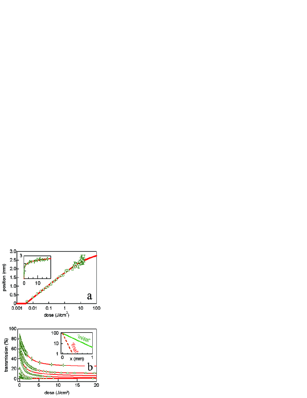
Figure 3: Experimental FPP results for an illustrative ‘partial photo-darkening’ polymerization. (a) Front position dependence on UV dose (light intensity exposure time) showing an initial logarithmic dependence followed by a crossover. The inset is a linear plot. (b) Optical transmission (up to 365 nm) variation during photocuring for PM samples of constant thickness. The inset depicts the log transmission as a function of thickness for the ‘initial’ (before conversion) and final (‘full conversion’) stages of photopolymerization, where the simple Beer-Lambert law holds, yielding the asymptotic $\mu_{0}$ and $\mu_{\infty}$ attenuation coefficients.

The optical transmission of this specific PM decreases during photocuring and this process is captured in Fig. 3b for a series of specimens with different thickness. There is clearly a drop in $Tr$ upon photopolymerization indicating partial photodarkening. The figure inset shows the thickness-dependent transmission before (‘initial’) and after (‘final’) a long UV exposure (until Tr reaches a plateau), in the usual Beer-Lambert representation. Other photoresists ‘photobleach’ during the process, due to consumption of a strongly absorbing species (generally the photoinitiator), or may remain virtually ‘invariant’ (with constant light transmission) upon conversion. The experimental results presented in Fig. 3 characterize the general nature of FPP and illustrate the kinetics of its observables, front position $h(t)$ and transmission $Tr(x,t)$, in a ‘photodarkening’ material.

IV Frontal Photopolymerization (FPP) Model

Photopolymerization begins with the absorption of light, which generates the reactive species responsible for chain initiation. The addition of a strongly light-absorbing photoinitiator modifies the optical properties of the medium and its consumption in the course of network formation, in conjunction with network formation and the formation of photopolymerization by-products, leads to an evolving optical attenuation. The consumption of the photoinitiator alone can be expected to lead to a reduction of the optical attenuation in the UV frequency range (‘photobleaching’), but the resulting polymer network can have an increased optical attenuation so that the net optical attenuation can increase upon photopolymerization (‘photodarkening’). Moreover, the addition of nanoparticle additives will also change the optical properties of the medium from those of the unfilled material in a non-trivial fashion.Cabral and Douglas (2005) We thus develop a model of photopolymerization that does not presume either photobleaching or photodarkening as a general consequence of photopolymerization. The nature of the polymerization front development has distinct features in these physical situations that we discuss in separate sections below after summarizing our general model.

The kinetic model of FPP Cabral et al. (2004); Cabral and Douglas (2005) conceives of the photopolymerization process in terms of a coarse-grained field theoretic perspective. The state of the material is assumed to be characterized by field variables that describe the extent to which the material is polymerized and the spatially and temporally dependent optical attenuation evolves in response to the photopolymerization process. While this model has mathematical similarities with classic theories of photo-polymerization Wegscheider (1923); Mauser (1967), it directly focuses on observable properties of FPP rather than the concentration of the various chemical species involved. The main variables of interest in the kinetic model are the FPP front position $h(t)$, as defined, for example, by the solid/liquid interface, the light transmission $Tr(x,t)$ of the PM layer and the optical attenuation constants ($\mu_{0}$, $\mu_{\infty}$) of the monomer and the fully converted material, respectively. The extent of polymerization $\phi(x,t)$ is then introduced as an ‘order parameter’ describing the extent of conversion of the growing polymerization front. The field variable $\phi(x,t)$ describes the average ratio of photopolymerized to unpolymerized material at a depth $x$ (the illuminated surface defines the coordinate origin) into the PM and satisfies the limiting relations $\phi(x,t\rightarrow 0)=0$ (no polymer) and $\phi(x,t\rightarrow\infty)=1$ (full polymerization) for all $x>0$. The second field variable $Tr(x,t)$ describes the optical transmission of the photopolymerizable medium of thickness $x$ at time $t$. This coarse-grained description of the photopolymerization front propagation has analogies with phase-field descriptions of ordering processes such a crystallization and dewetting where propagating fronts are also observed Warren and Boettinger (1995); Ferreiro et al. (2002).

The evolution of the photopolymerization process is modeled by introducing appropriate rate laws for the specified minimal set of field variables Cabral et al. (2004); Cabral and Douglas (2005). The rate of change of $\phi(x,t)$ is taken to be proportional to the optical transmission $Tr(x,t)$, the amount of material available for conversion and the reaction conversion rate $K$,

$$\frac{\partial\phi(x,t)}{\partial t}=K\left[1-\phi(x,t)\right]Tr(x,t)$$ (1)

Once photopolymerization has commenced, the material is considered to be a two-component system (consisting of reacted and unreacted material) whose components do not generally have the same optical attenuation coefficient $\mu$. The non-uniformity of the conversion profile will generally give rise to an effective attenuation factor $\bar{\mu}(x,t)$, which depends on thickness during conversion. Only before photocuring and near full conversion $\bar{\mu}(x,t)$ becomes constant. In our mean-field model, we postulate that the material can be described using a spatially varying and temporally evolving average optical attenuation,

$$\bar{\mu}(x,t)\equiv\mu_{0}\left[1-\phi(x,t)\right]+\mu_{\infty}\phi(x,t),$$

where ($\mu_{0}$) and ($\mu_{\infty}$) are the attenuation coefficients of the unexposed monomer and fully polymerized material, respectively. The variation leads to an evolution in the light intensity (or transmission) profile with depth according to the generalized Beer-Lambert relation,

$$\frac{\partial Tr(x,t)}{\partial x}=-\bar{\mu}(x,t)Tr(x,t),$$ (2)

where the usual Beer-Lambert law for a homogeneous material, $Tr(x,t)=\exp(-\bar{\mu}x)$, is recovered for short and long times as $\bar{\mu}(x,t\rightarrow 0)=\mu_{0}$ and $\bar{\mu}(x,t\rightarrow\infty)=\mu_{\infty}$.

Specific boundary conditions must be specified in order to solve such differential equations. Initially $\phi(x,0)=0$, while at the incident surface of the sample ($x=0$), we have no attenuation, thus $Tr(0,t)=1$. These are sufficient to determine unique solutions to Eqs. (1) and (2). We should also note that we can quickly solve Eq. (1) when $x=0$ to obtain

$$\phi_{0}(t)\equiv\phi(0,t)=1-\exp(-Kt),$$ (3)

an expression for the polymerized fraction at the edge of the sample that is independent of all model parameters except $K$.

The idealization of FPP evolution modeled by Eqs. (1) and (2) neglects the fact that numerous chemical components are actually generated in the course of photopolymerization and ignores the presence of additives and impurities that are often present in the photopolymerizable material. Additionally, it assumes simple chemical kinetics, defined by a single constant $K$. Thus, it is not clear a priori whether such a simple order parameter treatment of FPP is suitable. Judgement of the adequacy of our approach must be decided by comparison to measurements performed over a wide range of conditions. We next consider the final basic observable property of the FPP process, the position of the photopolymerization front.

As in ordinary gelation, we can expect solidification to occur once $\phi$ exceeds a certain ‘critical conversion fraction’ $\phi_{c}$ ($\ll$1). Since the liquid material can be simply washed away after any exposure time, the height $h(t)$ at which $\phi(x,t)=\phi_{c}$ indicates the surface of the photopolymerized material after curing and washing. This defines the position of FPP front in a concrete way and we adopt it below. Our previous measurements have shown that $\phi_{c}$ tends to be rather small [$\phi_{c}\sim\emph{O}(0.01)$] in our thiol-ene photopolymerizable material Cabral et al. (2004); Cabral and Douglas (2005) and this property is expected to be rather general. A small $\phi_{c}$ can be understood from the fact that solidification in polymerizing materials Lee and McKenna (1988) (e.g., ‘superglue’) normally involves a combination of glass formation and gelation, since the glass transition temperature strongly increases upon polymerization of a low molecular weight monomer. Accordingly, we adopt the representative value $\phi_{c}=0.02$ in our discussion below.

Equations (1) and (2) define a system of non-linear partial differential equations whose solution depends on three material parameters: the short and long-time attenuation coefficients, as well as the conversion rate $K$. The former two parameters can be measured independently with a series of transmission measurements of unpolymerized and fully polymerized specimens of different thicknesses. $K$ is determined by the polymerization chemistry and is a structural variable, yet both can be obtained as fitting parameters. The former has been the focus of much of the previous research Rytov et al. (1966); Terrones and Pearlstein (2001a, b); Terrones and Pearlstein (2003, 2004); Ivanov and Decker (2001); Goodner and Bowman (2002); O’Brien and Bowman (2003); Miller et al. (2002); Belk et al. (2003); Cramer et al. (2002, 2003); Reddy et al. (2003); Wegscheider (1923); Mauser (1967), and is not discussed in the present paper.

The coupled non-linear differential Eqs. (1) and (2) have not yet been solved analytically, apart from special limits that are briefly summarized in the next section. These exactly solvable cases include ‘total photobleaching’ where $\mu_{0}>0$ and $\mu_{\infty}=0$ and ‘photo-invariant polymerization’ in which the optical properties of the medium do not change in the course of polymerization (i.e., $\mu_{0}=\mu_{\infty}\equiv\bar{\mu}$). Front propagation is quite different in these different physical situations and we briefly describe the nature of FPP in these limiting cases, and then explore the full solution in some other physically relevant cases, where we identify those basic features of FPP that can be recognized experimentally. Rytov et al. Rytov et al. (1966) is one of few previous papers to study these different types of FPP, both by analytic modelling and experiment. This work, however, had to introduce rough approximations to obtain estimates of front properties.

V Exact Formal Solution of Kinetic Equations in Limiting Cases

V.1 Total Photobleaching
($\mu_{0}>0$ and $\mu_{\infty}=0$)

The initiator of the photopolymerization reaction often absorbs light strongly and the absorption of radiation can expected to lead to a reduction of the optical attenuation upon UV radiation through the chemical degradation of this reactive species. If this was the only species contributing to the optical attenuation of the medium, then the photopolymerized material would become increasingly transparent to light, becoming perfectly transparent to the radiation at infinite times. This is evidently an idealized model of photopolymerized materials, but most theoretical discussions of photopolymerization Decker (1998, 2002); Rytov et al. (1966); Terrones and Pearlstein (2001a, b); Terrones and Pearlstein (2003, 2004); Ivanov and Decker (2001); Goodner and Bowman (2002); O’Brien and Bowman (2003); Miller et al. (2002); Belk et al. (2003) are restricted to this limiting case based on the assumption that the PM initiator dominates the optical attenuation.

The case of perfect optical absorption is one of the few cases in which an exact solution can be expressed in terms of elementary functions, and this solution is instructive into basic features of FPP. In this case, the PM has a positive attenuation constant ($\mu_{0}>$ 0) and the attenuation of the polymerized material equals, $\mu_{\infty}=0$. In this case, Eqs. (1) and (2) can be easily solved to find that the conversion fraction $\phi(x,t)$ for perfect photobleaching equals Cabral and Douglas (2005)

$$\phi(x,t)=\frac{1-\exp(-Kt)}{1-\exp(-Kt)+\exp(\mu_{0}x-Kt)}.$$ (4)

Note that this expression reduces to Eq. (3) when $x=0$, and that the conversion fraction is defined solely for $x>0$. Eq. (4) was obtained long ago by Wegscheider Wegscheider (1923), but the physical interpretation of these equations differs in his treatment which models the concentration of reactive species, rather than the extent of photopolymerization.

Equation (4) can be written equivalently in terms of the coordinate $z$ moving with the front as,

$$\phi(z,t)=1/\left[1+\exp(\mu_{0}z)\right]=\frac{1}{2}\left(1+\tanh\left(\frac{\mu_{0}z}{2}\right)\right)$$ (5)

$$z=x-x_{f},\ x_{f}=\left[Kt+\ln\left[1-\exp(-Kt)\right]\right]/\mu_{0},$$ (6)

where $x_{f}$ is the inflection point of the front that propagates in space as the front advances. This position can also be identified in this model by a mathematically equivalent condition $\phi=1/2$, and the front position can thus can be defined by a (unique) maximum in $-\partial\phi(x,t)/\partial x=\phi_{x}$,

$$\left.\frac{\partial^{2}\phi}{\partial x^{2}}\right|_{x_{f}}=0.$$ (7)

The position $x_{f}$ is particularly applicable as a definition of the interface location if optical methods are used to probe the position of the front. Alternatively, as described in the previous section, it is sometimes more useful to define the front position by a ‘critical’ value of the order parameter $\phi(x,t)=\phi_{c}$ (e.g., value of $\phi$ at which the material becomes a solid). This front definition Cabral et al. (2004); Cabral and Douglas (2005); Hirose et al. (1990) leads to a travelling wave solution whose displacement also obeys Eq. (6).

Indeed, if we define a new coordinate $z_{h}=x-h(t)$, and insist that $\phi(z_{h}=0)=\phi_{c}$, we determine $h(t)$ as,

$$h(t)=x_{f}+\frac{1}{\mu_{0}}\ln\left(\frac{1}{\phi_{c}}-1\right).$$ (8)

Using the representative value of $\phi_{c}=0.02$ introduced above, we plot $h(t)$ in Fig. 5. The offset between our two interface position choices is then $\mu_{0}(h-x_{f})\approx 3.892$, for this example.

Equation (6) implies that $\phi(x,t)$ evolves as a propagating sigmoidally-shaped front whose position is defined by $x_{f}$. Since this profile will be compared with $\phi$ profiles for the general solution of Eqs. (1) and (2) below, we plot $\phi(z)$ in Figure 4 (the photo-invariant profile is discussed in the following section).

Figure 4: Conversion fraction $\phi$ as a function of z for both total photobleaching (solid) and photo-invariant polymerization (dotted), with $\mu_{0}=1.0$ mm^-1.

The position of this front $x_{f}$ (defined here by the inflection point, or $\phi=1/2$) is shown in Fig. 5. At long times ($t\gg K^{-1}$), the front translates linearly in time with a constant velocity $K/\mu_{0}$. Linear front propagation has commonly been reported in experimental studies of FPP kinetics (e.g., Rytov et al. (1966)).

At early times the position of the inflection point lies outside the polymerizing sample. Specifically, Eq. (3) implies $\phi(0,t)=1-\exp(-Kt)$, which can be less than $\phi=1/2$, the value of $\phi$ at the inflection point. The inflection point appears after an induction time,

$$\tau=\frac{\ln 2}{K},$$ (9)

which explains the intercept of the interface position shown in Fig. 5.

Figure 5: Plots of $x_{f}$ [mm] (emerging after an induction time $Kt\approx 1$) and $h(t)$ [mm] (emerging with little induction time at $Kt\rightarrow 0$) as a function of $Kt$ for both total photobleaching (solid) and photo-invariant polymerization (dotted), for $\mu_{0}=1.0$ mm^-1. At late times the total photobleaching position has a linear slope, corresponding to a front velocity of $K/\mu_{0}$

From our definition of the position of the FPP front, the width of the front $\xi$ can be correspondingly defined as the reciprocal of the magnitude of $\phi_{x}$ at the front position,

$$\xi\equiv 1/\left|\phi_{x}(x_{f})\right|$$ (10)

This definition is suitable for any symmetric front shape for which $\phi(x,t)\approx 1/2$ at the inflection point and we note that $\phi(x_{f},t)$ exactly equals $1/2$ for total photobleaching.

The light transmission $Tr$ is similarly exactly calculated as a function of either ($x,t$) or ($z,t$) as

$$Tr(x,t) = \left[{1-\exp(-Kt)+\exp(\mu_{0}x-Kt)}\right]^{-1};$$ (11)

$$Tr(z,t) = \frac{\phi(z)}{1-\exp(-Kt)}$$ (12)

This expression reduces to the Beer-Lambert relation, $Tr(x,t\rightarrow 0^{+})=\exp[-\mu_{0}x]$ for the photopolymerizable material at short times and $Tr(x,t)$ itself frontally propagates into the medium with increasing time. [$Tr(x,t)$ for air is unity in our model so that $Tr(x<0,t)\equiv 1$.] All of space thus becomes ‘transparent’ to radiation (i.e., $\mu$ = 0) in the limit of infinite times for total photobleaching, i.e., $Tr(x,t\rightarrow\infty)=1$. We plot $Tr(x,t)$ for representative dimensionless times $Kt$ in Fig. 6.

Figure 6: Time evolution of $Tr(x,t)$ as a function of $x$ for both total photobleaching (dotted) and photo-invariant polymerization (solid), for $\mu_{0}=1.0$ mm^-1. The total photobleaching case is shown for dimensionless times of $Kt=1,5,10,15$ and 20 (moving from left to right). At long times and large $x$, the slope of $\ln Tr$ approaches $1/\mu_{0}$, while for $x\rightarrow 0$ the slope of $\ln Tr$ approaches $1/\mu_{\infty}$ [see Eq. (2)].

V.2 Photo-Invariant Polymerization
($\mu_{0}>0$ and $\mu_{\infty}=\mu_{0}$)

Another important limit of our FPP model involves the situation in which the optical attenuation of the polymerized medium is taken to be unchanged from the pure monomer. This situation is a reasonable approximation if the monomer is the predominant component of the photopolymerizable material and if its optical properties (and density) are insensitive to conversion. In this photo-invariant polymerization case, the conversion fraction equals

$$\phi(x,t)=1-\exp[-K\exp(-\mu_{0}x)t].$$ (13)

As in the previous limiting case, note that this expression reduces to Eq. (3) when $x=0$. (Curiously, $1-\phi(x,t)$ is the Gumbel function Gumbel (1958) of extreme value statistics.) Eq. (13) can be written in the coordinate frame $z$ of the moving front as,

$$\phi(z,t) = 1-\exp[-\exp(-\mu_{0}z)]$$ (14)

$$z\equiv(x-x_{f}), x_{f}=\frac{\ln(Kt)}{\mu_{0}},$$ (15)

and we have plotted $\phi(z)$ and $x_{f}$ for this limiting case in Figs. 4 and 5. We note that $x_{f}$ is the position of the inflection of $\phi(x,t)$, and $\phi=1-e^{-1}\approx 0.632$ at this point. We see from this plot that $\phi(x,t)$ once again has an invariant sigmoidal shape.

As before, we define the height $h(t)$ of the FPP front by the condition $\phi(h,t)=\phi_{c}$:

$$\phi_{c}=1-\exp[-K\exp(-\mu_{0}h)t]$$ (16)

and we infer that the height $h(t)$ of the front grows logarithmically with time [see Eqn. (15), and Cabral et al. (2004)]

$$h(t,\mu_{0},K,\phi_{c}) = \frac{\ln(t/\tau)}{\mu_{0}}$$ (17)

$$\tau(K,\phi_{c}) \equiv \frac{\ln[1/(1-\phi_{c})]}{K}$$ (18)

This logarithmic front movement is contrasted with the linear frontal kinetics of the perfect photobleaching case. The expression for $h(t)$ in Eq. (17) is restricted to $t>\tau$ since the solidification front does not form instantaneously with light exposure, but grows at $x=0$ as dictated by Eq. (3). Thus, an induction time $\tau$ is required for $\phi$ to first approach $\phi_{c}$ and for the front to begin propagating. The magnitude of the induction time depends on the selected threshold $\phi_{c}$, becoming much larger for $x_{f}$ as $\phi_{c}$ approaches $\phi$ at the inflection point, $\phi_{f}$ [see Eq. (18)]. Notice that the slope of the $\ln(t)$ factor, describing the growth of $h(t)$ in Eq. (17), depends only on the optical attenuation $\mu_{0}$ rather than the rate of reaction and that the intercept governing the initial front growth is governed by $\tau$, which in turn depends on the rate constant, optical intensity and $\phi_{c}$. Such travelling wavefronts with a logarithmic displacement in time occur in diverse contexts Ben-Naim et al. (2001); Majumdar (2003). Our measurements of FPP with a thiol-ene photopolymerizable material have generally indicated logarithmic front displacement over appreciable time scales (see Fig. 3 and Cabral et al. (2004); Cabral and Douglas (2005)).

The transmission $Tr(x,t)$ does not evolve in time for photo-invariant polymerization; $Tr(x,t)$ simply decays exponentially with depth ($x$) according to the Beer-Lambert relation, $Tr(x,t)=\exp(-\mu_{0}x)$. This invariance with time is contrasted in Fig. 6 with the wave-like propagation of $Tr(x,t)$ in the photobleaching case, corresponding to the invasion of the polymerizable material of attenuation $\mu_{0}$ by an optically transparent medium.

It is important to realize that Eq. (17) describes the initial FPP growth process for an arbitrary optical attenuation of the polymerized material ($\mu_{0}>0$). Moreover, Eq. (17) describes the long time asymptotic growth provided that $\mu_{0}$ is replaced by its non-vanishing counterpart $\mu_{\infty}$ for the fully polymerized material. These extremely useful approximations arise simply because $\mu(x,t)$ is slowly varying in these short and long time “fixed-point” limits. The crossover between these limiting regimes can be non-trivial and is addressed below. In many practical instances, however, the time range is restricted to the initial stage governed by Eq. (17).

V.3 General FPP solution

Previous investigations of FPP have relied on numerical solutions of the governing kinetic equations in comparison to FPP measurements validating the model. These treatments were sufficient to demonstrate a good consistency between the model and experiment Cabral et al. (2004); Cabral and Douglas (2005), but many aspects of the model are difficult to infer in the general case without a full analytic treatment of the problem.

First, we define the transform variables $\theta=-\ln(1-\phi)$ and $\delta=-\ln(Tr)$. Eqs. (1) and (2) are then rewritten as

$$\frac{\partial\theta}{\partial t}=Ke^{-\delta},$$ (19)

and

$$\frac{\partial\delta}{\partial x}=\mu_{\infty}-(\mu_{\infty}-\mu_{0})e^{-\theta}.$$ (20)

We now take the $x$-derivative of Eq. (19) and the $t$-derivative of Eq. (20) and subtract the resulting equations obtaining

$$\frac{\partial^{2}}{\partial x\partial t}(\delta-\theta)=\mu_{\infty}\frac{\partial\theta}{\partial t}.$$ (21)

This equation can be integrated directly, yielding

$$\frac{\partial}{\partial x}(\delta-\theta)=\mu_{\infty}\theta+c_{1},$$ (22)

where $c_{1}(x)$ is an arbitrary function of $x$. We now impose the first of two boundary conditions: namely that at $t=0$, $\phi=0$ for all $x$ so $\theta(x,0)=0$, while $\delta(x,0)=\mu_{0}x$. This implies that $c_{1}(x)=\mu_{0}$, a constant. If we now insert Eq. (20) into Eq. (22) we find

$$\frac{\partial\theta}{\partial x}=(\mu_{\infty}-\mu_{0})\left(1-e^{-\theta}\right)-\mu_{\infty}\theta,$$ (23)

which again can be integrated. This integration gives

$$x=\frac{1}{\mu_{\infty}}\int^{\theta}_{\theta_{0}}\frac{d\theta^{\prime}}{\lambda\left(1-e^{-\theta^{\prime}}\right)-\theta^{\prime}},$$ (24)

where we define $\lambda\equiv 1-\mu_{0}/\mu_{\infty}$ and impose the second boundary condition $\theta_{0}=Kt$ (see Eq. 3.) Note that $\theta_{0}$ is the dimensionless time introduced above. An expression for $\theta$ is obtained by defining the auxiliary function, $\cal J_{\lambda}(\theta)$,

$${\cal J_{\lambda}(\theta)}\equiv\int^{\theta}_{1}\frac{d\theta^{\prime}}{\lambda\left(1-e^{-\theta^{\prime}}\right)-\theta^{\prime}}.$$ (25)

Although ${\cal J_{\lambda}}(\theta)$ is non-standard, it can be readily determined as with other, more familiar, special functions. The existence of an inverse function of ${\cal J_{\lambda}}(\theta)$ is guaranteed if $\lambda<1$, which is assured by the physics of the problem (since this restriction simply implies $\mu_{0}>0$). Insight into ${\cal J}_{\lambda}(\theta)$ is found by noting that for large values of its argument, ${\cal J}_{\lambda}(\theta)$ is well approximated by,

$${\cal J_{\lambda}}(\theta)\approx{\cal J_{\lambda}}(C)+\ln|\lambda-C|-\ln|\lambda-\theta|.$$ (26)

where $C\gg 1$ is a point of expansion. For small values of the argument we can develop another expansion about $c\ll 1$

$${\cal J_{\lambda}}(\theta)\approx{\cal J_{\lambda}}(c)+\frac{\ln(c)}{1-\lambda}-\frac{1}{1-\lambda}\ln\theta.$$ (27)

For much of the range of its arguments,

$$\left({\cal J}_{\lambda}(\theta)-\mathrm{const}\right)\propto\ln(\theta).$$

We can now rewrite Eq. (24) as

$$\mu_{\infty}x={\cal J_{\lambda}(\theta)}-{\cal J_{\lambda}}(Kt).$$ (28)

Eq. (28) fully solves the problem, since we can now write $\theta(x,t)$ formally as

$$\theta(x,t)={\cal J_{\lambda}}^{-1}(\mu_{\infty}x+{\cal J_{\lambda}}(Kt));\quad\phi(x,t)=1-e^{-\theta}.$$ (29)

Note that the dependencies upon $x$ and $t$ are fully separated, implying a functional invariance in the propagation of the $\phi$ interface’s shape. We explore this invariance in detail below.

We can also solve for $Tr$, using the formal solution to Eq. (2)

$$Tr(x,t)=\exp\left\{-\int_{0}^{x}dx^{\prime}\left[\mu_{0}(1-\phi(x^{\prime},t))+\mu_{\infty}\phi(x^{\prime},t))\right]\right\}.$$ (30)

Remarkably, this can integrated to fully solve the problem:

$$Tr(x,t)=\frac{\lambda\phi+\ln(1-\phi)}{\lambda\phi_{0}+\ln(1-\phi_{0})}=\frac{\lambda\phi+\ln(1-\phi)}{\lambda(1-e^{-Kt})-Kt}.$$ (31)

The solutions for the basic measurable variables $\phi(x,t)$ and $Tr(x,t)$ are now formally complete. Using any simple mathematical software the above solutions can be implemented, solved and plotted.

V.3.1 Shape of the interface

Based on our experience with the two limiting cases of total photobleaching and photoinvariant polymerization, we expect the interface shape to be sigmoidal. We now analyze the solution in an effort to determine its general properties, without reference to particular parameter choices. We know that $\phi(x,t)$ should increase at any fixed position as $t$ increases. From Eq. 23 we can easily find $\partial\phi/\partial x$ as,

$$\frac{\partial\phi}{\partial x}=\mu_{\infty}(1-\phi)\left[\lambda\phi+\ln(1-\phi)\right].$$ (32)

Since $\lambda\leq 1$ and $\mu_{\infty}>0$, we see that $\partial\phi/\partial x$ is always less than $0$. This is our first observation about the shape of the curve: its slope is such that $\phi$ monotonically decreases as $x$ increases. Our second observation comes from Eq. (3), where we see that $\phi_{0}=\phi(0,t)$ rises from $0$ to $1$ as $t$ increases, while $\phi(x\rightarrow\infty)$ approaches $0$. We also note that since $\phi$ monotonically decreases as $x$ increases, $\phi_{0}$ is the time-independent maximum value of $\phi$. This property derives from the invariance of $\phi(x)$ interface shape in time (see below).

As for the two limiting cases, the shape can be further examined by computing the inflection point of $\phi$, e.g. the extremum of $\partial\phi/\partial x$:

$$\frac{\partial^{2}\phi}{\partial x^{2}}\propto\lambda(1-2\phi_{f})-1-\ln(1-\phi_{f})=0,$$ (33)

where $\phi_{f}$ is the value of $\phi$ at the inflection point. It is interesting that the value of $\phi_{f}$ at the inflection point can be determined by an equation involving elementary functions, while the determination of the position of this point, $x_{f}$, requires the use of our auxiliary function ${\cal J}_{\lambda}$. If we desire, we can compute $\theta_{f}$ using $\theta_{f}=-\ln(1-\phi_{f})$. Note that for physical values of $\lambda<1$, there is only one solution to Eq. (33). This unique value of $\phi_{f}$ can exceed the maximum value of $\phi$, which occurs, as noted above, at $\phi(0,t)$. In this case the plot of $\phi(x,t)$ has no inflection point. Once the induction time $t>-\ln(1-\phi_{f})/K$ has passed, then the inflection point exists for positive values of $x$.

Thus, we have a detailed picture of the interface profile characteristics:

1. The maximum value of $\phi(x,t)$ at any given time is always at $x=0$, and this maximum value, $\phi_{0}=\phi(0,t)$, rises in time as $\phi_{0}=1-\exp(-Kt)$ .

2. Both $\phi$ and $\partial\phi/\partial x$ approach 0 when $x\rightarrow\infty$.

3. $\partial\phi/\partial x<0$ for all values of $x$, thus $\phi$ decreases monotonically with increasing $x$.

4. There is a single extreme value of the slope $\partial\phi(x,t)/\partial x$. This extremum is found when $\phi=\phi_{f}$ as dictated by Eq. (33), but only when $t>-\ln(1-\phi_{f})/K$.

This description outlines precisely the sort of sigmoidal shape we expected based on our physical understanding of the system.

V.3.2 Position of the interface

We next explore the properties of the above solution for $\phi(x,t)$ in as much generality as possible. Eq. (28) is particularly illuminating, since it can be rewritten as

$$z\equiv x-x^{*} = \frac{1}{\mu_{\infty}}{\cal J_{\lambda}}(\theta)-x_{0}$$ (34)

$$x^{*} = x_{0}-\frac{1}{\mu_{\infty}}{\cal J_{\lambda}}(Kt),$$ (35)

where we now see that the shape of the interface is invariant in time, as it was in the limiting cases, and propagates with the position $x^{*}(t)$. Indeed, we can invert Eq. (34) and write

$$\theta(z)=-\ln(1-\phi(z))={\cal J}_{\lambda}^{-1}(\mu_{\infty}(z+x_{0}))$$ (36)

While we are free to choose any value of the offset of the interface position $x_{0}$, several choices present themselves. One is the position of the inflection point $x_{f}$, defined by the solution to Eq. (34) with $\theta=\theta_{f}$, found from Eq. 33. If we set $x^{*}=x_{f}$ we then have the formal equations describing the interfacial positions,

$$x_{0} = \frac{1}{\mu_{\infty}}{\cal J_{\lambda}}(\theta_{f}),$$ (37)

$$x_{f} = \frac{1}{\mu_{\infty}}\left({\cal J_{\lambda}}(\theta_{f})-{\cal J_{\lambda}}(Kt)\right)$$ (38)

We can get more insight into the properties of this inflection point by calculating the solution to Eq. (33) for all $\lambda\in(-\infty,1]$. Both $\theta_{f}$ and $\phi_{f}$ vary over a fairly narrow range, as is seen in Fig. 7, where $\phi_{f}\in[0.5,~{}0.797]$ and $\theta_{f}\in[\ln 2,~{}1.594]$.

Figure 7: Plot of $\theta_{f}$ (solid upper curve) and $\phi_{f}$ (dotted lower curve) as a function of $\lambda$. In the limit $\lambda\rightarrow-\infty$, $\phi_{f}\rightarrow 0.5$ and $\theta_{f}\rightarrow\ln 2$.

As was done in the limiting cases, we can also define the “height function” $h(t)$, by choosing a particular value of $\phi=\phi_{c}$ which marks the interface position. With this choice, and the relation $\theta_{c}=-\ln(1-\phi_{c})$, we then have the formal expressions

$$x_{0} = \frac{1}{\mu_{\infty}}{\cal J_{\lambda}}(\theta_{c}),$$ (39)

$$h(t) = \frac{1}{\mu_{\infty}}\left({\cal J_{\lambda}}(\theta_{c})-{\cal J_{\lambda}}(Kt)\right).$$ (40)

The only difference between $x_{f}$ and $h$ is the fixed ‘offset’

$$h(t)-x_{f}=\frac{1}{\mu_{\infty}}\left({\cal J_{\lambda}}(\theta_{c})-{\cal J_{\lambda}}(\theta_{f})\right).$$ (41)

V.3.3 Induction time

In our study of the limiting cases, we found an induction time when $\phi(x,t)$ first exceeded $\phi_{f}$ (at the inflection point) or $\phi_{c}$ (the physically selected interface position). In general, regardless of what convention we choose for the interface position, the induction time will be simply the solution to $\phi_{0}=\phi^{*}$, where $\phi^{*}$ is the value of $\phi$ at the interface $\phi_{f}$ or $\phi_{c}$. Using Eq. (3) this is simply

$$\tau=\frac{-\ln(1-\phi^{*})}{K}$$ (42)

Because of this induction time, and the different values of $\phi^{*}$ used in our definitions of $x_{f}$ and $h$, these functions can actually behave quite differently at early times. Typically we select $\phi_{c}\ll 1$, and thus, for this case, the induction time will be relatively short on experimental time scales, $\tau\approx\phi_{c}/K$. On the other hand, our computation of the range of $\phi_{f}\in(0.5,0.797)$ implies a range in $\tau\in(0.693,1.594)$. These values of $\tau$ are between 35 and 80 times larger than induction times established using a typical choice of $\phi_{c}=0.02$.

V.3.4 Approximations to the front position

It is useful to obtain approximate expressions for Eq. (34). At early times we can develop an approximation solely for $h$, since $x_{f}$ is undefined at early times. Using Eq. (27) we obtain the explicit estimate

$$h(t)\approx\frac{1}{\mu_{0}}\ln\left(\frac{Kt}{\theta_{c}}\right);\ \theta_{c}<Kt\ll 1$$ (43)

Thus, an early time log-linear plot of $h(t)$ will yield a slope of $1/\mu_{0}$. Note that this expression is exact for the case of photo-invariant polymerization, as comparison with Eq. (18) reveals.

At long times, we can develop a general expression for an approximate form to $x^{*}$ using Eq. (26). Thus, we introduce an expansion for the limit $C\gg 1$,

$$x^{*}\approx x_{0}-c_{1}+\frac{1}{\mu_{\infty}}\ln|\lambda-Kt|$$ (44)

where $c_{1}=[{\cal J}_{\lambda}(C)+\ln|\lambda-C|]/\mu_{\infty}$.

We recall, however, the limiting case where $\mu_{\infty}=0$ (total photobleaching) yields,

$$x^{*} = x_{0}+\frac{1}{\mu_{0}}\left[Kt+\ln\left(1-e^{-Kt}\right)\right],$$ (45)

$$x_{0} = \frac{1}{\mu_{0}}\ln\left(\frac{1}{\phi^{*}}-1\right),$$ (46)

which has a linear $x^{*}\propto t$ behavior at long times. This seems quite different from the logarithmic behavior given above for the general expression. How can this be understood? In the limit $\mu_{\infty}\rightarrow 0$, we have that $\lambda\rightarrow-\infty$. For any non-zero value of $\mu_{\infty}$ the logarithmic behavior the approximate form must dominate at long times. However there will always be an intermediate time (perhaps a very long time if $|\lambda|$ is large!) when $Kt\ll|\lambda|$, and in this case we can expand the $\ln|\lambda-Kt|\approx\ln|\lambda|-Kt/\lambda$ to obtain linear behavior.

$$x^{*}\approx x_{0}-c_{1}+\frac{Kt}{\mu_{0}-\mu_{\infty}}+\frac{\ln|\lambda|}{\mu_{\infty}};\ 1\ll Kt\ll|\lambda|$$ (47)

Now that we have a “general” solution to our kinetic equations, we examine the specific cases of partial photodarkening and partial photobleaching.

V.4 Illustration of general solution: partial photobleaching vs. photodarkening

The limits of perfect photobleaching and photo-invariant polymerization are ideals that only approximately arise in practice. In general, the optical attenuation of the polymerizable material is always greater than zero and can either increase or decrease upon conversion.

It is possible that the reactive products generated by the photoinitiator or the polymerization of the monomer increase the optical attenuation so that the polymerized material becomes increasingly opaque to radiation with increasing time: partial photodarkening ($\mu_{\infty}>\mu_{0}$). We find that this is a common situation in our FPP measurements, regardless of the presence of nanoparticles, or temperature variations Cabral et al. (2004); Cabral and Douglas (2005). For this case we choose the realistic model parameters: $\mu_{0}$ = 1 mm^-1, $\mu_{\infty}=5.0$ mm^-1, $K$= 1 s^-1. As mentioned before, we select the representative value for $\phi_{c}$ = 0.02.

Figure 8: Evolution of the conversion $\phi$ with time for partial photodarkening (parameters in text), plotted (going up and leftward) at $Kt=$0.1, 0.5, 1.0, 1.40897, 5, 20, 50, 100, 1000, and 10000.

The spatio-temporal variation of the conversion fraction $\phi(x,t)$ is shown in Fig. 8 and its the derivative $-\partial\phi(x,t)/\partial x$ is shown in Fig. 9. (Since the slope is negative definite, we plot its magnitude $-\partial\phi/\partial x$). We see the development of a well defined advancing front as in the perfect photobleaching and photo-invariant limits, discussed above. We compare these results with other choices of the parameters below.

Figure 9: Evolution of $-\partial\phi/\partial x$ in time for partial photodarkening, shown (going up and left to right) at $Kt=$0.1, 0.5, 1.0, 1.40897, 5, 20, 50, 100, 1000, and 10000.

In contrast to photodarkening, we also consider the case where $\mu_{\infty}$ is small: partial photobleaching ($\mu_{\infty}<\mu_{0}$). Specifically, we keep all other parameters the same but reduce $\mu_{\infty}$ by a factor of 10. Thus, $\mu_{\infty}=0.5$ mm^-1, implying $\lambda=-1$. The behavior of this system should then be somewhere between the partial photoinvariant case and the total photobleaching limit.

Note that the frontal kinetics of FPP is specified by only 4 basic model parameters in the framework of our model: $\mu_{0}$, $\mu_{\infty}$, $K$ and $\phi_{c}$. The attenuation coefficients can be determined independently with a set of $Tr$ vs. thickness experiments of the neat and fully polymerized material (Fig. 3). $K$ may be determined by the time (or dose) dependence of the $Tr$, for various thicknesses. Finally, the solidification conversion threshold $\phi_{c}$ is obtained by fitting measurements of height as a function of dose to our theory.

We next consider a comparative analysis of the FPP front cases. The extent of polymerization conversion fraction $\phi$ propagates as a shape invariant waveform, after an induction period. The time evolution of $\phi$ for partial photodarkening is illustrated in Fig. 8 with parameters $\lambda=0.8$ and $\mu_{\infty}=5.0$. We find from Eq. 33 that $\phi_{f}=0.755605$, and therefore $\theta_{f}=-\ln(1-0.755605)=1.40897$. Accordingly, the shape of $\partial\phi/\partial x$, plotted in Fig. 9, is invariant for $Kt>1.40897$ and simply propagates to the right as $t$ increases. For the partial photobleaching case we find $\theta_{f}=0.852606$ and $\phi_{f}=0.573697$. This shape invariance is best understood and appreciated by transforming $\phi$ into the moving coordinate $z$ of the front (as in Fig. 4), which is shown below. First, however, we consider the time dependence of the position of the front. As before, the location of the peak in $\partial\phi/\partial x$ defines $x=x_{f}(t)$ [Eq. (38)]. We now see why $x_{f}$ is also a suitable alternative choice for the position of the FPP front (particularly if optical methods are used to locate the interface experimentally). Evidently, the peak height and shape of $\partial\phi/\partial x$ are invariant after the peak first appears at $Kt>\theta_{f}$.

Figure 10: Conversion $\phi(z)$ as a function of the coordinate in the moving frame of the front $z$ for 4 different cases: total photobleaching (solid, $\lambda=-\infty$), partial photobleaching (long-dash, $\lambda=-1.0$), photoinvariant (dotted, $\lambda=0$), and partial photodarkening (short-dash, $\lambda=0.8$). The plots were chosen so that they intersect at $\phi=\phi_{c}$. The profiles are time-invariant.

The time-invariant nature of the front propagation of $\phi$ in the moving frame is illustrated in Fig. 10. We observe that the $\phi(z)$ profiles are sigmoidal and independent of time when plotted with respect to the transformed variable $z=x-h(t)$. All curves intersect when $\phi=\phi_{c}$, explaining the overlap at low values of $\phi(z)$.

Since $x_{f}(t)$ and $h(t)$ are both important measures of FPP frontal kinetics, we compute these observable quantities in Fig. 11 for all four cases: total photobleaching (solid, $\lambda=-\infty$), partial photobleaching (long-dash, $\lambda=-1.0$), photoinvariant (dotted, $\lambda=0$), and partial photodarkening (short-dash, $\lambda=0.8$). In all cases, the interface evidently appears after its (dimensionless) induction time $Kt=-\ln(1-\phi^{*})$, where $\phi^{*}=\phi_{c}=0.02$ for the height $h$ (group emerging near $Kt\rightarrow 0$), while $\phi^{*}=\phi_{f}$ for the inflection point front position $x_{f}$ (group emerging near $Kt\approx 1$), where $\phi_{f}$ is found from Eq. (33). Note that the vertical offset between $x_{f}$ and $h$ is the constant $x_{0}$ dictated by Eq. (38). All the examples shown reach $x_{f},\ h\propto\ln Kt$ at late times (near where $Kt>|\lambda|$), except for total photobleaching, which remains in linear growth kinetics at late times.

Figure 11: Front position $x_{f}$ (emerging from the $Kt$-axis near $Kt\approx 1$) and $h$ (emerging as $Kt\rightarrow 0$) as a function of $Kt$. We show all 4 cases: total photobleaching (solid, $\lambda=-\infty$), partial photobleaching (long-dash, $\lambda=-1.0$), photoinvariant (dotted, $\lambda=0$), and partial photodarkening (short-dash, $\lambda=0.8$). The interface appears after its induction time $Kt=-\ln(1-\phi^{*})$, where $\phi^{*}=\phi_{c}=0.02$ for the plots of $h$ while $\phi^{*}=\phi_{f}$ for the case of $x_{f}$.

As in the total photobleaching case, we see that the FPP front position (as defined by the inflection point) is insensitive to crossover effects since this feature develops at late times (see Fig. 11). The displacement in time is logarithmic after a short induction time. The front position $h(t)\equiv x(\phi=\phi_{c})$, as defined by a ‘critical’ conversion (here, $\phi_{c}=0.02$), does exhibit a noticeable crossover. As anticipated from Eq. (5), the front position $h(t)$ moves logarithmically at ‘short’ times where $\bar{\mu}(x,t\rightarrow 0)\approx\mu_{0}$ and crosses over to a slope determined by $\bar{\mu}(x,t\rightarrow\infty)\approx\mu_{\infty}$, respectively, as the monomer interconverts to a polymerized network. In the partial photodarkening case, the front moves faster initially ($\propto 1/\mu_{0}$) and slows down ($\propto 1/\mu_{\infty}$) at later times. The situation occurs in the case of partial photobleaching.

The evolution of the light intensity is sensitive to the evolution of the optical attenuation and is thus particularly interesting and informative about the nature of the front development. The transmission $Tr(x,t)$ (dimensionless intensity profile) as a function of depth for various curing times is plotted in Fig. 12 for both sets of parameters. The initial profile is simply $Tr=e^{-\mu_{0}x}$, and it decreases in the manner given by Eq. (31). In the short and long time limits, we see that the usual Beer-Lambert law holds and the intensity decays exponentially in $x$, with attenuation coefficients $\mu_{0}$ and $\mu_{\infty}$, respectively. At intermediate times, there is a crossover between these two asymptotic regimes. Note that an attempt to fit experimental transmission results with the simple Beer-Lambert law would result in an unphysical ($\neq$ 1) intercept for infinitely thin films, symptomatic of the necessity of accounting for the variation in $\mu$ in the course of photopolymerization. This is how we first recognized the importance of partial photodarkening in our former measurements Cabral et al. (2004); Cabral and Douglas (2005).

Figure 12: Transmission $Tr(x,t)$ as a function of position at the late time of $Kt=10.0$, for 4 different cases: total photobleaching (solid, $\lambda=-\infty$), partial photobleaching (long-dash, $\lambda=-1.0$), photoinvariant (dotted, $\lambda=0$, and partial photodarkening (short-dash, $\lambda=0.8$). The slopes exhibit the expected crossover from $1/\mu_{0}$ to $1/\mu_{\infty}$. The frontal character of $Tr(x,t)$ is illustrated in Fig. 6 and Figs. 4 and 5 of Cabral and Douglas (2005).

Figures 10–12 summarize our findings for the conversion $\phi(z)$ and light attenuation $Tr(x,t)$ profiles, frontal kinetics (using both inflection $x_{p}$ and height $h$ criteria) for the four cases illustrated: total and partial photobleaching, photoinvariant and partial photodarkening polymerization. We see from this comparative discussion that, while the properties of polymerization front propagation in the unpolymerized material are general, the shape of the fronts $\phi$ and $Tr$ and the time development of the front position (linear and logarithmic, induction time) depends on the evolution of the optical attenuation upon polymerization.

VI Conclusions

We have exactly solved a model frontal photopolymerization (FPP) that directly addresses the kinetics of the growth front position and the change in optical attenuation in time under general circumstances. This model involves an order parameter $\phi(x,t)$ describing the extent of conversion of monomer to polymer (solid) and the extent of light attenuation, $Tr(x,t)$. Many aspects of the photopolymerization process derive from the changing character of the optical attenuation $\mu$ in the course of PM exposure to light, and we illustrate how this effect can lead to significant changes in the kinetics of front propagation.

The optical attenuation of the photopolymerizable material leads to non-uniformity in the extent of polymerization. Solidification develops first at the boundary when the polymer conversion becomes sufficiently high and then a front of solidification invades the photopolymerizable material in the form of a wave. We find that the interface between the solid and liquid is described by a polymerization density profile $\phi(z)$ whose shape is invariant in time. The time dependence of the front movement and the shape of $\phi(z)$ depend on the change of the optical attenuation accompanying polymerization. The position of the front is established using one of two methods: by specification of a critical value $\phi_{c}$ for which solidification occurs (a convenient definition for photolithography where the liquid material is simply washed away after photo exposure) or by determination of the inflection point in $\phi(z)$. We find that the initial frontal growth kinetics are logarithmic in time, governed by the optical properties of the unconverted material and are followed by a transient crossover. Front displacement in this crossover regime is complex, as it depends on whether conversion decreases or increases the optical attenuation. At long times, the front displacement becomes universally logarithmic in time (excluding the case of “perfect photobleaching” where the optical attenuation after UV exposure exactly vanishes and fronts propagate linearly in time), but it may take an (impractically) long time for this asymptotic behavior to be reached. Many of the asymptotic properties of the general case of evolving optical attenuation that we describe in our model are captured in a simplified model in which the optical attenuation is assumed to be a positive, non-vanishing constant: photo-invariant polymerization.

Our general treatment of photopolymerization has been found to quantitatively describe frontal growth in both neat Cabral et al. (2004) and nanoparticle filled Cabral and Douglas (2005) photopolymerizable materials (thiol-ene copolymers) and to capture the effect of temperature (through a single rate parameter) Cabral and Douglas (2005). This description provides a predictive framework for controlling the spatial dimension of photopolymerizable materials for microfluidics and other applications, where the rapid microfabrication of solid structures is required.

VII Acknowledgments

Support from the NIST Combinatorial Methods Center (NCMC) is greatly appreciated.

References

- Odian (1991) G. Odian, Principles of Polymerization (John Wiley & Sons: New York, 1991).
- Fouassier (1995) J.-P. Fouassier, Photoinitiation, Photopolymerization, and Photocuring (Hanser / Gardner Publications: Cincinnati, OH, 1995).
- Fouassier and Rabek (1993) J.-P. Fouassier and J. F. Rabek, Radiation Curing in Polymer Science and Technology (Elsevier Applied Science: London, 1993).
- Decker (1998) C. Decker, Polymer Int. 45, 133 (1998).
- Decker (2002) C. Decker, Polymer Int. 51, 1141 (2002).
- Harrison et al. (2004) C. Harrison, J. T. Cabral, C. Stafford, A. Karim, and E. J. Amis, J. Microeng. Micromach. 14, 153 (2004).
- Cabral et al. (2004) J. T. Cabral, S. D. Hudson, C. Harrison, and J. F. Douglas, Langmuir 20, 10020 (2004).
- Wu et al. (2004) T. Wu, Y. Mei, J. T. Cabral, C. Xu, and K. L. Beers, J. Am. Chem. Soc. 126, 9880 (2004).
- Cygan et al. (2005) Z. T. Cygan, J. T. Cabral, K. L. Beers, and E. J. Amis, Langmuir (2005).
- Hudson et al. (2004) S. D. Hudson, J. T. Cabral, W. Goodrum, K. L. Beers, and E. J. Amis, Appl. Phys. Lett. (2004).
- Khan and Pojman (1996) A. M. Khan and J. A. Pojman, Trends Polym. Sci. 4, 253 (1996).
- Pojman et al. (1996) J. A. Pojman, V. M. Ilyashenko, and A. M. Khan, J. Chem. Soc., Faraday Trans. 92, 2825 (1996).
- Lewis et al. (2004) L. L. Lewis, C. A. DeBisschop, J. A. Pojman, and V. A. Volpert, in Nonlinear Dynamics In Polymeric Systems (Eds. J. A. Pojman, Q. Tran-Cong-Miyata Q., pp. 169, ACS Symposium Series 869, 2004).
- Cabral and Douglas (2005) J. T. Cabral and J. F. Douglas, Polymer (2005).
- (15) Certain commercial equipment, instruments, or materials are identified in this paper in order to specify the experimental procedure adequately. such identification is not intended to imply recommendation or endorsement by the national institute of standards and technology, nor is it intended to imply that the materials or equipment identified are necessarily the best available for the purpose.
- Jacobine (1993) A. F. Jacobine, in Radiation Curing in Polymer Science and Technology (Eds. J.-P. Fouassier and J. F. Rabek, Vol. 3, Chapter 7, pp. 171, Elsevier Applied Science: London, 1993).
- Cramer et al. (2002) N. B. Cramer, J. P. Scott, and C. N. Bowman, Macromolecules 35, 5361 (2002).
- Cramer et al. (2003) N. B. Cramer, T. Davies, A. K. O’Brien, and C. N. Bowman, Macromolecules 36, 4631 (2003).
- Reddy et al. (2003) S. K. Reddy, N. B. Cramer, T. Cross, R. Raj, and C. N. Bowman, Chem. Mat. 15, 4257 (2003).
- Wegscheider (1923) R. Wegscheider, Z. Phys. Chem. CIII 103, 273 (1923).
- Mauser (1967) H. Z. Mauser, Naturforsch. B 22, 569 (1967).
- Warren and Boettinger (1995) J. A. Warren and W. Boettinger, Acta Metall. Mater. 43, 689 (1995).
- Ferreiro et al. (2002) V. Ferreiro, J. F. Douglas, J. A. Warren, and A. Karim, Phys. Rev. E 65, 051606 (2002).
- Lee and McKenna (1988) A. Lee and G. B. McKenna, Polymer 29, 1812 (1988).
- Rytov et al. (1966) B. L. Rytov, V. B. Ivanov, V. V. Ivanov, and V. M. Anisimov, Polymer 37, 5695 (1966).
- Terrones and Pearlstein (2001a) G. Terrones and A. J. Pearlstein, Macromolecules 34, 3195 (2001a).
- Terrones and Pearlstein (2001b) G. Terrones and A. J. Pearlstein, Macromolecules 34, 8894 (2001b).
- Terrones and Pearlstein (2003) G. Terrones and A. J. Pearlstein, Macromolecules 36, 6346 (2003).
- Terrones and Pearlstein (2004) G. Terrones and A. J. Pearlstein, Macromolecules 37, 1565 (2004).
- Ivanov and Decker (2001) V. V. Ivanov and C. Decker, Polymer Int. 50, 113 (2001).
- Goodner and Bowman (2002) M. D. Goodner and C. N. Bowman, Chem. Eng. Sci. 57, 887 (2002).
- O’Brien and Bowman (2003) A. O’Brien and C. N. Bowman, Macromolecules 36, 7777 (2003).
- Miller et al. (2002) G. A. Miller, L. Gou, V. Narayanan, and A. B. Scranton, J. Polym. Sci. A, Polym. Chem. Ed. 40, 793 (2002).
- Belk et al. (2003) M. Belk, K. G. Kostarev, V. Volpert, and T. M. Yudina, J. Phys. Chem. B 107, 10292 (2003).
- Hirose et al. (1990) T. Hirose, K. Wakasa, and M. Yamaki, J. Mater. Sci. 25, 1209 (1990).
- Gumbel (1958) E. J. Gumbel, Statistics of Extremes (Columbia University Press, New York, 1958).
- Ben-Naim et al. (2001) E. Ben-Naim, P. L. Krapivsky, and S. N. Majumdar, Phys. Rev. E 64, 035101 (2001).
- Majumdar (2003) S. N. Majumdar, Phys. Rev. E 68, 026103 (2003).