Sound modes broadening for Fibonacci one dimensional quasicrystals.
Abstract
We investigate vibrational excitation broadening in one dimensional Fibonacci model of quasicrystals (QCs). The chain is constructed from particles with masses and following the Fibonacci inflation rule. The eigenmode spectrum depends crucially on the mass ratio . For (what roughly mimics icosahedral () QCs) there are three almost dispersionless optic modes separated from the acoustic mode by three large gaps, for (what mimics -QCs) there is one dispersionless optic mode and one acoustic mode. We calculate also the eigenfunctions which near the gaps are deviated strongly from simple (Bloch-like) periodic functions. All calculations performed self-consistently within the regular expansion over the three wave coupling constant. The problem can be treated as well in the framework of the perturbation theory over the parameter which we formally consider as a small parameter. The approach can be extended to three dimensional systems. We find that in the intermediate range of mode coupling constants, three-wave broadening for the both types of systems (1D Fibonacci and 3D -QCs) depends universally on frequency and scales as (where and are constants). For smaller values of the coupling constant broadening turns out proportional to . Our general qualitative conclusion is that for a system with a non-simple elementary cell phonon spectrum broadening is always larger than for a system with a primitive cell (provided all other characteristics are the same).
pacs:
61.44.Br, 63.20.DjI Introduction
Extensive experimental and theoretical work on quasiperiodic systems (i.e. materials which exhibit non-periodic long-range order) has revealed interesting new properties which are not found in either periodic or in disordered systems (see e.g., CS86 - SR03 , the references we will quote in more details in what follows). One of the remarkable features of QCs, (e.g., revealed in neutron diffraction and inelastic scattering experiments) is the apparent conflict between the high structure quality of these materials and their vibrational excitations which are rather reminiscent of those for disordered materials CF03 , RF03 .
Although as it was mentioned already above, there is a considerable literature discussing eigenmodes and related properties of QCs, and a number of sophisticated calculations have been published over the last 20 years, there is still a clear need for a simple (but yet non-trivial) theoretical model with predictions which can be directly tested experimentally. For instance, results found by exact diagonalization of dynamical matrices at high symmetry points of the small Brillouin zone for corresponding QCs approximants (see e.g. HK93 ) lead to very rich density of vibrational states including many different modes. However there is still very limited correspondence between these theoretical studies and only two or three broad and almost dispersionless optical modes (besides acoustical phonons at smaller frequencies) observed in experiments BB93 , BB95 , BB99 , DB99 , SK02 . In part this frustrating situation is just due to the lack of a simple and tractable model, and the main goal of this paper is geared towards the building and testing of a simple model for vibrational modes in -QCs.
Our motivations for presenting this paper are twofold. First is based on a simple observation that a disallowed in conventional crystalline materials 5-th order rotational symmetry of -QCs determines the unique golden ratio of incommensurate length scales that completely defines the structure of all -QCs. As we will see in what follows that many robust and experimentally testable features of the excitation spectra in -QCs are sensitive to only this specific feature of the structure. Second - we go one step further with respect to the results known already in the literature (see, e.g., KC96 , LO86 ) providing in the present paper a systematic procedure for handling vibrational mode broadening in QCs. The broadening is often considered as a nuisance, while as we will show, it provides valued information on QC physical properties and eigenmode structure. To our knowledge such a calculation of the eigenmode broadening in QCs was not carried out thus far. The simplest model structure constructed by the same golden ratio is the 1D Fibonacci chain. Our aim is not to claim that the Fibonacci 1D model we propose necessarily holds for real 3D -QC materials but to analyze the model and to compare qualitatively its predictions with experimental data. Note, however, that all calculations can be performed self-consistently not only in 1D but as well can be generalized for 3D QCs. Besides we study the model within the regular expansion over the parameter , assuming that , where is some ”effective binary QC”(see its definition below in the section II) mass ratio. Of course our oversimplified model is only a zero approximation which may not have exactly right numbers but could lead to more or less right shapes of the dispersion laws. The reasonability of our assumptions, model and physics behind will be commented at various places in this paper.
Our paper is organized as follows. In the next section II we describe our model and calculate its vibrational spectrum. In section III we compute the eigenfunctions, and in section IV we find the mode broadening due to anharmonic three wave coupling. Finally we review and discuss our results in conclusion section V. In two appendices to the paper we collect some more specialized technical material required for the calculations phonon line broadening due to anharmonic third order processes for the 5-particle approximants to the infinite Fibonacci chain (appendix A) and three wave phonon broadening in isotropic 3D system with -space limited by the sphere (appendix B). Those readers who are not very interested in mathematical derivations can skip these appendices finding all essential physical results in the main text of the paper.
II Fibonacci Model
As it is well known a regular periodic 1D lattice can be generated from one basic unit cell by simple translation. For the ideal periodic system the solution of the equation of motion is wavelike and the vibrational spectrum forms one or more vibrational bands. The density of state is singular near these bands edges. In the opposite limit of the totally disordered lattice, the wave functions exhibit localization behavior, and one has only a discrete spectrum. The quasiperiodic lattices we are interested in this paper are intermediate in this sense between ideally periodic and totally disordered systems. To generate 1D quasiperiodic system one has to apply more general procedure. We are constructing the chain from particles with masses and in the following way (so-called the Fibonacci inflation rule):
| (1) |
and so forth such that the ratio [number of ]/[number of ] approaching the golden mean value (the same as for -QCs) in the limit of long sequences. A symmetrical inflation rule and can be also used to generate a Fibonacci chain where the roles of majority and minority basis are exchanged. To determine the phonon spectrum of the Fibonacci chain we have to solve the dynamic equations for every atom ( is the displacement of the -th atom):
| (2) |
Here and below we employ the units with elastic moduli equal to unity. Of course it is impossible to solve (2) analytically for an arbitrary chain, with more than 4 particles, therefore numerical methods should be used to investigate the system.
The computations can be performed in many ways. For example one can find the vibrational spectrum using the standard transfer matrix formalism LO86 . However, predominantly aiming to analyze mode broadening, we will use here another approach seems to be more appropriate for our purposes. First of all it is more convenient instead of the infinite Fibonacci chain to study the finite chain of the length with zero boundary conditions for the displacements , and to have the spectrum for the infinite chain, the results should be computed in the limit . For the conventional 1D crystal, i.e. we easily obtain the well-known spectrum
| (3) |
In the long wavelength limit, , the details of the quasiperiodic structure do not play a significant role for vibrational spectra (unlike electronic spectra), and therefore we get in this limit the same spectrum (3). Evidently it is not the case for finite and . Let us chose to be more specific and somehow in contact with real -QCs. Almost all known -QCs are three component alloys, for example, , , where superscripts indicate the mass number of the element and subscripts show the atomic concentration of the element in the alloy. Unfortunately with the Fibonacci chain we can mimic simply only two component alloys. However, luckily the mentioned above -QCs alloys roughly contain one more light component and two more heavy components, and for the both -QCs we have the mass ratio between the average heavy and the light component about at the composition for , and the mass ratio is at the composition for . We conclude that the composition in the both cases is not very different from the golden ratio, therefore the Fibonacci chain approximation at least in this respect might serve quite reasonable.
To have a nontrivial solution for the particle displacements , the eigenmode frequency must satisfy the eigenvalue equation. The latter one, e.g., in the transfer matrix technique, is the condition that the determinant of the product of transfer matrices should be zero. It allows to find easily the phonon spectrum of the Fibonacci chain (see e.g. KC96 , LO86 ). The spectrum has gaps which may be labeled by the so-called Bloch index ( is the golden mean ratio) and the size of the gaps decreases roughly with increasing . The model exhibits characteristics of both a regular periodic and a disordered system. In the low-frequency region, the system behaves as a regular periodic crystals (and the vibrational eigenfunctions appear extended), in the high-frequency region, there is no unique behavior for the eigenfunctions, and the spectrum shows many gaps. However the exact solution is, so to speak, too exact for our purposes, and contains too many subtle details of the model such as the hierarchical nature of gaps, and all branches of excitations simultaneously, while experimentally observed spectra measured at room temperature are much more poor, and it is not clear whether it is possible at all to observe or to test experimentally these theoretically predicted features of the spectra and to find somehow their characteristics. For -QCs and , for which detailed studies have been carried out BB93 , BB95 , BB99 , DB99 , SK02 , vibrational excitation spectra can be separated into two well defined regimes: the acoustic regime for frequencies smaller than, say, and, for larger frequencies, a regime in which the dynamical response is characterized by a broad band of dispersionless optic-like modes. The optic like spectrum generally consists of 3 or 4 broad ’bands’ (a few wide), and no any gap opening is observed. That is all and, therefore, aiming to understand underlying basic physics and to model even qualitatively observed dependences, one should not refine the model to include some additional mechanisms and details, but just to the contrary, one has to coarse - grained the model, to have a benchmark to compare theoretical predictions and experimental data.
One more comment is in order here. Of course real -QCs are not one-dimensional Fibonacci chain. However the one-dimensional and three-dimensional problems share a common mathematical foundation based on the golden mean ratio , the both systems can be obtained by a projection method from a higher dimensional space (two dimensional square lattice for the Fibonacci model KN84 ), and it is not surprising that they have common quite robust and generic universal properties. As it is the case in related electronic problems RM97 , RB03 we expect the qualitative features of the spectra will carry over to two- and three-dimensional cases, and similar results hold for any irrational . Moreover phonon line broadening, our main concern in this paper, is even more robust phenomenon in QCs than the spectrum itself. Indeed for QCs we have deal with infinitely many density modulation harmonics, filling densely the reciprocal space. However one always can separate a major series of density modulation harmonics, and the corresponding wave vectors scale like , thus depending mainly on universal QC building blocks ratio. Due to this fact though formally the number of relevant states which are in resonance with any given one is infinite, the most of these harmonics have very small amplitudes, and therefore their resonances are irrelevant in our coarse - grained approach. The same can be seen by comparing characteristic time scale of the processes responsible for the line - broadening. For the particular density modulation, the time of energy () transfer is of the order of . Thus when the scattering is dominated by a fast three wave anharmonic coupling we are investigating in this paper, there is no time for an effective influence of the other resonances due to small harmonics of the QC density modulation. Although in this study we are mainly concerned with 1D systems, to support aforesaid qualitative arguments we presented in the appendix B the generalization of our approach to three dimensional systems.
Let us recapitulate the results of our analysis of the 1D Fibonacci chain vibrational modes. The following conclusions are deducted from the numerical solution of the eigenvalue equation, we present in the Fig. 1.
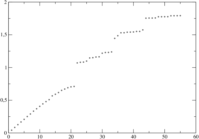
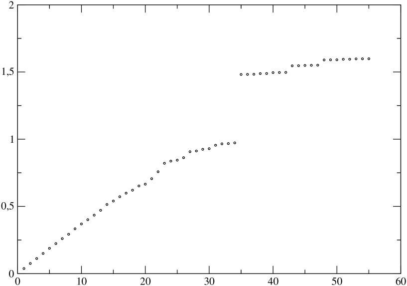
The eigenmodes for 55 particles in the elementary cell shown in Fig.1, computed with zero displacement boundary conditions and for the mass ratio 1:3. Evidently one can distinguish one acoustic branch and optical branches. Qualitatively the same features of the spectrum occur also for 233 or 1000 particles. Let us first consider the case when the mass ratio is about 1:3 and the composition is about 38:62, which can mimic -QC . By a simple coarse-grained (!) inspection of the results of such calculations we find that in this case we have 3 optical modes with rather weak dispersion, one acoustic mode and one ”quasi-optical” mode next to the acoustic one. The gap between the acoustic branch and the first quasi-optical mode is relatively small, much smaller than the other 3 gaps. Analogously for the composition 62:38, the spectrum has only 2 branches, one acoustic and one optic mode, the latter one is almost dispersionless (Fig.2).
The described above method (zero boundary displacements) widely used in the literature (see e.g. KC96 ) is adequate if one is looking for only the spectrum, however, the method is failed for the consideration of anharmonic three wave contributions into mode broadening, what is our calculations ultimate aim. It is evident in the limit . Indeed in the case the eigenfunctions are simply -functions and clearly the mean product of any three functions is always zero. For this product is not zero any more, but it turns out very small. Thus to analyze eigenfunctions and anharmonic contributions for the Fibonacci chain one must use a different approach to describe vibrational modes. For example we can take 5 (remind that 5 is the Fibonacci number) particles in the elementary cell and impose non zero periodic boundary conditions, requiring that phases of the displacements within the elementary cell, are confined in the interval from to . In the standard solid state physics language it is the same as the introduction of quasi-momenta in the first Brillouin zone (evidently for 5 particles in the elementary cell and periodic boundary conditions the introduced phase is the quasi-momentum up to the constant factor). Luckily it occurs that the spectrum calculated in this simple model in the harmonic approximation practically coincides with the spectrum obtained by the previous method, although formally the both spectra are expressed in different variables:
-
•
in the former approach the spectrum consists from the discrete points; every mode can be characterized by a certain number corresponding to a certain mode numeration, (it could be, see, e.g., KC96 , the the eigenfunction nodes number), and the spectrum is one per one correspondence between these numbers and computed eigenfrequencies;
-
•
in the latter approach the phase plays the role of a wave vector (which strictly speaking is undefined in the previous approach since in the Fibonacci model there are no Bloch states).
Therefore now we have 5 modes (eigenfrequencies) which can be represented as the functions of the phase or quasi-momentum. The fact that the both spectra are fairly closed (see Fig.3) is not an accidental coincidence. It is based on a described above natural generalization of the notion of wave vectors for the quasiperiodic systems. Even more we will see in the next section that in the limit of small frequencies the eigenfunctions of the Fibonacci chain vibrational spectrum are practically indistinguishable from the Bloch-like waves, thus one should expect that the displacement phases (or the quasi-momenta) are reminiscent of the mode numbers.

A similar behavior is obtained for the next approximant in the series. As we proceed by considering higher order approximant to the Fibonacci chain, new gaps progressively appear in the spectrum, showing a hierarchical scaling structure. However, all corse-grained global features of the spectrum remains the same as for very short approximants to infinite quasiperiodic chains.
III Eigenfunctions
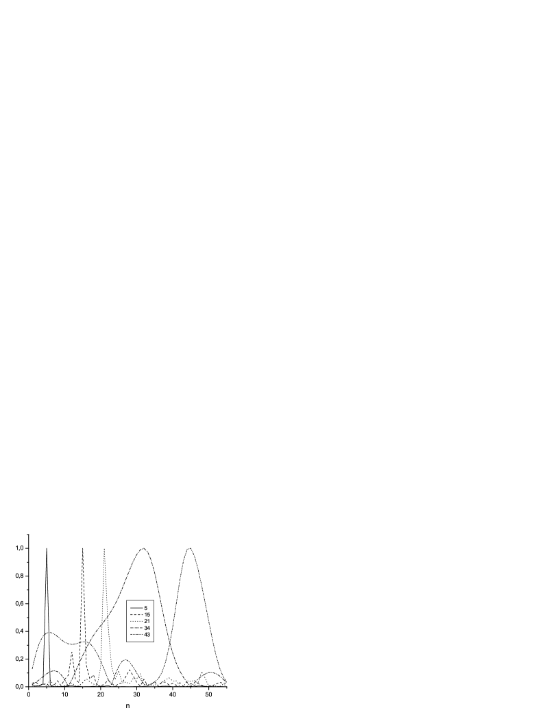
As it is well known if the system is periodic, Bloch’s theorem may be applied, and the solutions of (2) are wavelike, propagating ones. On the contrary, if the lattice is disordered, the eigenfunctions are localized, and the spectrum is a discrete set of levels. Common sense suggests that since the Fibonacci chain is intermediate between periodic and disordered systems, it is expected to show the both characteristics. Let us first consider the eigenfunctions for the discrete point-like spectrum (i.e. the eigenfrequency as the functions of mode numbers). For the small eigenfrequencies the eigenfunctions are similar to the Bloch-like periodic functions. For the particular case of zero boundary conditions these eigenfunctions can be written as . Near the gaps the eigenfunctions are represented as certain linear combinations of the periodic functions, i.e., the wave packets. The spectral width of any of the wave packet is proportional to the value of the gap. The most broad eigenfunctions are at the boundaries of the gaps, and the values of eigen numbers at the gaps are the corresponding Fibonacci numbers. The largest gaps occur for the mass ratio 1:3 at the positions after 2,3,4 elements (for the case when the unit cell length is 5). We illustrated some features of the eigenfunctions in the Fig. 4 where we presented Fourier transforms of 5 typical eigenfunctions for a chain with 55 particles in the elementary cell. From this simple figure important conclusions are arrived at. Namely as it was already noticed above for small eigen numbers the eigenfunctions only slightly differ from periodic Bloch-like ones. However near the gaps the eigenfunctions are strongly deviated from the Bloch solutions and they describe localized or intermediate (critical) states.
To clarify further the situation few remarks are in order here:
-
•
Since the eigenfunctions are not Bloch-like periodic ones, in the thermodynamic limit, () there is no the quasi-momentum conservation law;
-
•
The eigenfunctions near the large gaps have quite broad widths in the reciprocal () space, the spectral distributions of the neighboring eigenfunctions are strongly overlapped. Having in mind neutron measurements it can lead to the situation when some phonon branches are disappeared at certain values and the next branch can appear at the lower quasi-momentum value;
-
•
We note that in all published reasonably accurate inelastic single grain neutron scattering experiments, BB93 , BB95 , BB99 , DB99 , SK02 , the predicted gaps in the vibrational spectra, have not been detected. One can attribute this failure to the mode broadening, which could be larger than the corresponding gaps. However, say the natural broadening, related to the fact that the calculated above eigenfunctions have a finite width in space, is rather small and can not close the big gaps between the optical modes. Therefore one has to include the other broadening mechanisms, and the most relevant one is associated with three phonon interactions LL81 .
IV Three wave broadening
As it was shown in the previous section, that already 5 particles ordered as give the phonon spectrum qualitatively and semi-quantitatively quite close to the spectrum of the large Fibonacci chain. Evidently, for the 5 particles in the elementary cell system, one has 5 branches of the excitations: one acoustic branch (1), one optical mode (2) with non-zero dispersion close to the acoustical mode, and three optical almost dispersionless (3,4,5) modes. For the mass ratio the simple analysis of the spectrum lead to the following not-forbidden anharmonic three phonon processes:
Actually only some parts of the corresponding branches can participate in these three phonon interactions. Indeed, for example, the processes with two phonons from the dispersionless optical modes and one phonon from the acoustic or from the first optical mode are allowed only for the small for the latter mode. All other processes between such phonons are forbidden. Thus we conclude that soft phonons with small wave vectors do not participate in these three phonon processes and, therefore, in this approximation such phonons have no broadening at all. This observation is conformed with known results of inelastic neutron scattering measurements close to the strong Bragg peaks, which show that there is a characteristic wave vector of the order of , such that only for the sound modes exhibit broadening BB93 , BB95 , BB99 , DB99 , SK02 .
IV.1 Basic model
Just to illustrate the point and our calculation scheme, let us first consider the elementary cell with 2 atoms, and . All allowed three wave processes depend strongly on the value of . For the only possible anharmonic process is the decay of the optical phonon with and into the two phonons with . For smaller one has a certain finite region (not only one point) within the optical mode where this kind of three wave processes is not forbidden. To study the three wave phenomena more rigorously one should start with the vibrational Hamiltonian of the system including third order anharmonic terms. The Hamiltonian can be written as LL81
| (4) |
Here are the creation or annihilation operators of the corresponding phonons, is the three wave coupling potential, the integration is performed over the first Brillouin zone, means the complex conjugated contribution, and the summation is performed over all branches of the phonon spectrum (for the simplest model with two particles in the elementary cell, these are one acoustic and one optical branch).
We calculate the simplest one-loop correction to the phonon spectrum. Since the expansion in the Hamiltonian (4) is over the triple phonon interaction vertex can be presented as . Note that actually the interaction vertex has also some smooth dependence on the wave vectors which can be found only numerically. Therefore, to illustrate the essential physics by a simple picture, in the paper we neglect this dependence.
According to the general principles of quantum statistical physics LL81 , the probability of a phonon decay, (i.e. the vibrational mode broadening, we are interested in) can be calculated self-consistently from the Hamiltonian (4). To do it one has to introduce certain bare decrements ( for the simplest model with two particles into the elementary cell) into the phonon eigenstates. As a result we get the following self-consistency Born integral equations
| (5) | |||
where . Our main concern here is the case where the phonon broadening is rather large, therefore the thermal phonon excitations giving dominate contributions into the broadening should be thermally occupied, i.e. ( is Debye temperature), as it is the case in the experimental inelastic neutron scattering investigations BB95 , DB99 , SK02 we have in mind in this paper. Thus in the condition we replace the Bose energy level occupation factor by the Boltzmann distribution function in the high temperature limit. The solutions of these equations can be easily found numerically, and we presented the results in Fig 5.
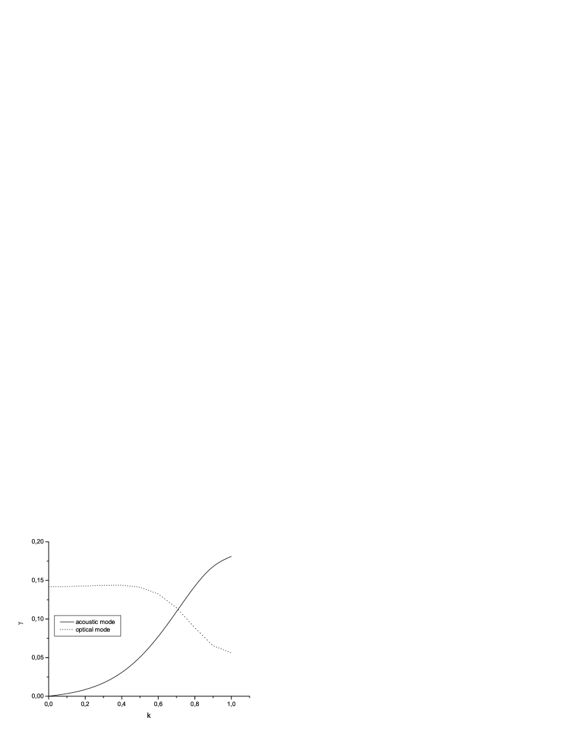
One might think that the equations (5) do not contain any QC-specific feature of the system, but it is only partially true. In fact the mode broadening (5) is determined by the key QC property, namely, a finite band of almost dispersionless optic modes interacting with the acoustic phonon. On the same footing the aforesaid statement is applied in our approach, to any system with a non-simple unit cell. Indeed the low-lying optical modes from approximant crystals might be practically indistinguishable from quasi-local modes. The broadening depends (at a given mass ratio ) on the mode coupling parameter , i.e. it is non universal. It is worth noting also quite peculiar behavior for the optical mode broadening decreasing for . The physics behind can be rationalized as follows. For a given mass ratio about the conservation laws prohibit the three wave interactions of the type for the optical phonons with the wave vectors . This broadening reduction phenomenom is even more pronounced for the smaller coupling constant (as it is demonstrated below in Fig. 7).
To illustrate this non universality we show in Fig. 6 the calculated three wave broadening for a relatively large anharmonic coupling ( in our dimensionless units).

The results in this case (strong coupling) can be fitted by law. For a small coupling constant broadening law is quite different, as we show in Fig. 7, where ). In the both cases the mass ratio was taken , which mimics two kinds of -QCs we described above.
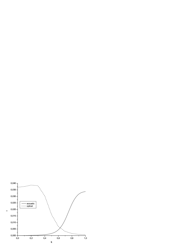
The figures 6 and 7 manifest clearly that dependence does not hold for small anharmonic coupling, and besides the figures show the difference between the regions of parameters corresponding to forbidden and allowed three wave processes. It is worth noting that the three wave anharmonic coupling on the relevant in (5) length scales may be in fact much larger than anharmonic contributions conventionally measured by macroscopic (e.g. specific heat) methods SF02 , SL02 ).
We have shown already in section II that the global structure of the vibration spectrum for quasiperiodic chains can be obtained in practice by considering very short approximants to infinite chains. For the Fibonacci chain, the reasonable size approximant imitating the infinite QC system contains 5 particle in the elementary cell, which is with our choice of masses (). Note in passing that the same statement is true also for electronic spectra RM97 , RB03 . Although the generalization of the presented above analysis and results for two particles in the elementary cell to the unit cells with five atoms is conceptually straightforward, it deserves some precaution, as it implies tedious and bulky calculations, which could be done analytically only under certain rather restrictive approximations. Appendix A to the paper contains basic methodical details and equations necessary for these calculations, and besides it gives a way to construct a regular method for calculating higher order perturbative corrections. Here in Fig. 8 we present only the results of our analysis for the 5-atom elementary cell.

Only the main three-wave processes , , , , are taken into account at the computation, and besides, for the sake of simplicity and having in mind published inelastic neutron scattering experimental data BB93 , BB95 , BB99 , DB99 , SK02 , all in the range above Debye temperature, we assume the classical (Boltzmann) statistics of the vibrational excitations.
Fig. 8 shows that the decrement for the lowest first acoustic branch tends to zero for small wave vectors (as it should be), and that the higher energy mode broadening are in the same range of magnitudes (of the order of in our dimensionless units). Remembering that in the same units characteristic inter-mode spacing (i.e. their eigenfrequency differences) we found in section II is about we come to the following conclusions:
-
•
due to the broadening in the range of resonances between acoustic and optic modes the sound mode can no longer be described as a single excitation;
-
•
large broadening of the acoustic phonon modes is related to the three wave mechanism;
-
•
the very existence of several quiet broad optical modes in QCs can be understood as an illustration that in QCs there are many ways in which the neighboring configurations can be arranged, as a result a single level, which initially was the same for all configurations becomes a band of the modes;
-
•
there are at least two main reasons why three phonon processes lead to much more noticeable contributions to sound absorption in QCs (more precisely in the systems with non-simple unit cells) in comparison with conventional crystals. First for the QC there is a dense set of umklapp vectors, and second there are almost dispersionless optic modes possessing finite widths, and a large phase volume in the reciprocal space is available for the acoustic phonons interacting with the optical modes.
-
•
in own turn this noticeable broadening might be a reason why no forbidden gaps have been observed experimentally.
Few more words on umklapp processes seem appropriate here. As it is a textbook wisdom, the total momentum of any set of interacting particles in a periodic crystal need only be conserved to within a wave vector from the reciprocal lattice. The fundamental role of these so-called umklapp processes is to open further scattering channels where the momentum of the particles in the initial state is different from that of the final state. In a QC its reciprocal space contains all the necessary wave vectors to match any required frequency conversion processes. However this striking fact is almost irrelevant for the linear phenomena since the corresponding susceptibilities anyway should remain constant in space. Evidently it is not the case for non-linear susceptibilities and processes, like three wave interaction, which as we illustrate in the frame work of our model can be enhanced noticeably in the quasiperiodic systems.
IV.2 Refinement of the basic model
Presented in the previous subsection results can be extended in many ways. First, for the sake of a skeptical reader we have to admit that strictly speaking our calculations are not self consistent ones. Indeed in our approach (5) (see also (9) in the appendix A) we have taken into account only three wave processes which are not forbidden in the zero temperature limit. By other words it means that there is no bare phonon mode broadening. For finite temperatures and non-zero bare phonon decay, the other processes could be also relevant, and the most important processes are , because the spectrum of acoustic phonons is approximately linear for small wave vectors (i.e., ), which always allows three phonon interactions. Therefore in the case of finite (and, in fact, not small) temperatures, we have to add the contributions corresponding to these processes into the right-hand side of the first Equation (5) (or for 5-particle elementary cell into the r.h.s. of (9)). We presented in the Fig. 9 the phonon broadening with such a contribution taken into account (for the magnitude of the coupling vertex ).

A nice feature of this contribution is that the shape of the acoustic branch decrement occurs almost independent of the magnitude of (for the interaction constant larger than the threshold which is about 0.005, see Fig. 10).
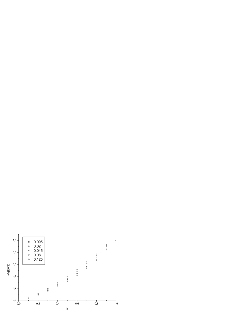
One more note of caution is in order here. In the previous subsection we replaced the Bose distribution function by the classical occupation factor . Luckily the acoustic branch broadening will not change its shape depicted in the Fig. 10 up to the temperature larger than the maximum phonon energy in the acoustic branch. Thus our approximation holds as well in a quite broad range of temperatures.
This universal contribution into the acoustic mode broadening can be also analyzed analytically, and it illustrates several characteristic features of the phenomenom. We believe that the phonon decrement is significantly smaller than its frequency. To simplify consideration we assume also that the decrements of the optical modes do not depend on or , i.e. those aquire the constant values. Experimental data and our numerical investigations show that optical phonon decrements indeed only very weakly depend on the wave vectors. Replacing in the first equation in (9) , ( as above is the sound speed), we are facing to solve the integral equation
| (6) | |||
Since the decrement is assumed to be small in comparison with the frequency it is possible to replace frequencies differences in the numerators in the following way
| (7) |
Evidently the first three terms give the broadening proportional to . The fourth term for the positive values is determined mainly by the integration region , where its denominator is minimal. The last term can be transformed into the same form after the replacement . Eventually this equation can be rewritten as
| (8) |
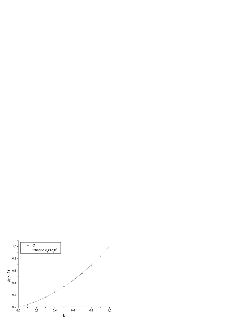
where and are numerical coefficients. The last approximate equality in (8) is obtained after the first iteration in (8). Thus we end up with the following universal analytical form for the acoustic mode decrement . This simple expression fits very well computed numerically function (see Fig. 11).
In order to provide a more complete account of the vibrational broadening phenomena, similar analysis has been performed to include self consistently the potentially relevant processes ( is the vibrational branch number, and as before corresponds to the acoustic mode). We closely follow the same procedure as above for the broadening and thus skipping all details presented only the results in Fig. 12.

It turns out that these new processes have little effect on the acoustic branch decrement, and the broadenings of all other branches only weakly depend on the wave vector and increase monotonically with the branch number. A result that justifies the assumptions made above, and proves that our model includes all ingredients necessary to capture the correct broadening effects in the Fibonacci chain.
IV.3 Self consistent expansion over the parameter .
Thus we investigated the Fibonacci lattice based on the golden ratio (and to confront our results with known and well studied -QCs the mass ratio was ) as an example of the quasiperiodic 1D systems. There are many other non periodic structures which are nonetheless fully deterministic and in this sense highly ordered. Qualitatively the same behavior one can expect also in 1D incommensurate systems. With this remark in mind it is interesting and instructive to extend the analysis of the previous section for a quasiperiodic system with the mass ratio chosen to make use of the smallness of the parameter . If this assumption is granted we can apply a regular expansion over the small what allows us to study even the infinite chain.
To move further on smoothly let us remind the characteristic features of the Fourier spectrum for periodically repeated finite Fibonacci block (remind that the length of the elementary cell is a Fibonacci number also). According to the Nyquist theorem (see e.g., WE83 ) for particles in the elementary cell one can determine only independent Fourier harmonics. The absolute value of each of the Fourier amplitude is an even function of its wave number. The zero wave number harmonic has the largest amplitude. The next large amplitude harmonics have numbers and , with the ratio close to the golden ratio . The next by their amplitudes harmonics have the wave numbers and so on. For example, for the wave numbers of the highest harmonics are . Evidently the amplitudes of all harmonics with non-zero wave numbers are proportional to the small parameter , the corresponding proportionality coefficients are approximately constant and the constant is smaller than one. The amplitude ratio of the different harmonics is independent of the small parameter , and for the first two main harmonics (except the zero harmonic) this ratio is about .
Armed with this knowledge we are in the position now to consider the phonon spectrum in such a system. For particles in the elementary cell we get the spectrum with one acoustic and optical branches. The gaps between the branches are determined by the amplitudes of corresponding Fourier harmonics. The amplitude of the harmonic, say, with the wave number determines two spectral gaps with the numbers and respectively. Noting that the sum of these two gaps is approximately equal to the amplitude of this harmonic, we arrive at the conclusion that the vibrational spectrum of the Fibonacci chain possesses the sequence of the gaps, and the value of the gap depends on its wave number and the parameter . In the limit all gaps also tend to zero. The chain turns into the crystalline Bravais lattice with the only one particle in elementary cell and the only one acoustic phonon branch. For finite but small values of the parameter the difference between the phonon spectra of the quasiperiodic system under consideration and the corresponding Bravais lattice should be also small. To be more specific let us focus on the simplest non Bravais system with three particles in the elementary cell. The main feature of this non Bravais lattice is that the length of Brillouin zone is three times smaller than for its Bravais counterpart, and besides there are two additional non zero Fourier harmonics. The acoustic branch of the non Bravais lattice practically coincides with the corresponding part (one third) of the acoustic branch of the Bravais lattice. However, the optical branches in the non Bravais lattice spectrum are significantly different. Let us denote by the size of the Brillouin zone for the Bravais lattice. For the optical modes we easily get that and , where is the only phonon frequency in the Bravais lattice. Three wave interaction in the Bravais lattice is determined by a certain vertex , which supposed to be not very different from the similar triple interaction vertex between the acoustic phonons for the non Bravais lattice. However in the non Bravais case we have to consider also all other interactions which include the optical phonons. We denote the corresponding vertex , because it describes in fact the four wave coupling, and is the Fourier amplitude of the density modulation at the wave vector . Actually the vertex can also be reduced to , and therefore the natural estimate for the vertices is .
The number of the wave vectors entering into the vibrational thermal broadening is equal to the number of the optical modes. Thus for our simple case with three particles in the elementary cell we have deal with two vectors, and their Fourier amplitudes are equal and proportional to . Furthermore the effective triple vertex in the main over approximation and including all not forbidden processes can be written as
Finally the thermal vibrational mode broadening is determined by the square of this vertex. In a general case the different contributions into do not interfere. Let us remind again that this conclusion is based on our assumption of , what is equivalent to say that the amplitudes , are small, and non small Fourier harmonics are included in the basic structure (as we did above for the harmonic with the wave vector ).
Now we can compare the thermal broadening for the Bravais and non Bravais cases. The only three wave process allowed in the Bravais lattice is evidently . For the non-Bravais case we have besides it also the three wave processes related to the interaction vertex . For our simplest case with three particles in the elementary cell and the both additional vertices coincide and proportional to . One can see that the vibrational broadening for the non Bravais case always exceeds the broadening in its Bravais counterpart. The corresponding difference of the both decrements is proportional to the value (for the sake of simplicity we consider to be a constant). We present the results in Fig. 13 for the and . The qualitative inescapable message of this is that the phonon broadening is always larger for a non-simple elementary cell (in comparison to the corresponding simple Bravais elementary cell).

V Conclusion
In conclusion, in this paper we examine one important (and overlooked in previous investigations) aspect of QC vibration spectra, namely - line broadening. We concentrate on the broadening mechanisms which are intrinsic to the structure of QCs, i.e. those that would be present at any dimension of QCs, and even in a hypothetical defect-free materials. To understand physics, underlying the QC dynamics, we studied first the simplest case - one-dimensional Fibonacci chain. As it is well known facts if the system is periodic, the Bloch theorem LL81 may be applied and, therefore, the solution of the equation of motion is wavelike, the phonon spectrum forms one or more bands, and the density of states is singular near the band edges. On the other hand, if the lattice is totally disordered, the eigenfunctions exhibits localization phenomena, and the spectrum is a discrete set. The QC structure is intermediate between between the ideal periodic and disordered, so it shows characteristic of both systems. For example in the low frequency limit , the spectrum in our coarse-grained approximation appears as continuous because the widths of gaps become smaller than the separation of the eigenmodes in a chain of finite length.
Let us now add a few more ingredients en root to some tentative conclusions. Our model chain is constructed from particles with masses and following the Fibonacci inflation rule. As the length of the pattern goes to infinity, the ratio between the total number of elements of different components approaches constant value. The eigenmode spectrum depends crucially on the mass ratio . For (what roughly mimics -QC ) there are three almost dispersionless optic modes separated from the acoustic mode by three large gaps. For (what mimics -QCs) there is one dispersionless optic mode and one acoustic mode. All calculations performed self-consistently within the regular expansion over the three wave coupling constant. The problem can be treated as well in the framework of the perturbation theory over the parameter which we formally consider as a small parameter. We find noticeable three wave anharmonic contributions into the spectrum, i.e. to the mode broadening. The broadening depends (at a given mass ratio ) on the mode coupling constant, and for relatively strong coupling, is proportional to ( is wave vector transmitted to the mode). The need of an exponent lower than 4 for -dependent line broadening (very often attributed to Rayleigh scattering in disordered materials CF03 , RF03 ) to fit the thermoconductivity data in -QC was indicated also in KC96 . However, the line broadening dependence on wave vectors turns out not universal one. The acoustic mode decrement for the coupling parameter higher than the exponent of the power law becomes smaller than 3, and for very small coupling this kind of power law fitting becomes inadequate. We expect that found for 1D Fibonacci chain robust features of the vibrational spectra will carry over to two and three dimensional cases. To illustrate this statement we extended our approach also to three dimensional systems. We find that in the intermediate range of mode coupling constants, three-wave broadening for the both types of systems (1D Fibonacci and 3D -QCs) depends universally on frequency and scales as (where and are constants). It is instructive to compare these predictions with the results known for say standard (i.e. possessing simple Bravais unit cells) crystalline materials, where the inelastic anharmonic processes lead to a temperature dependent linewidth which scales as , whereas elastic scattering of the Bloch like waves by the static inhomogeneities leads to a temperature independent linewidth proportional to in 3D systems. Our general qualitative conclusion is that for a system with a non-simple elementary cell phonon spectrum broadening is always larger than for a system with a primitive cell (provided all other characteristics are the same). Although our model is a toy model in the sense of caricaturizing some physical features (like, e.g., three wave broadening), when properly interpreted, it can yield quite reasonable values for a variety of measured quantities. Our model establishes the universal properties of the vibrational spectra associated with generic features of any system with a non-simple unit cell.
Acknowledgments
We thank M. de Boissieu and R. Currat for the numerous discussions inspired this work. One of us (E.K.) acknowledges support from INTAS (under No. 01-0105) Grants.
Appendix A
The system of equations for phonon line broadening in the 5- particle approximant to the infinite Fibonacci chain, reads
| (9) |
Here only the main three-wave processes , , , , are taken into account and besides we assume classical statistics for the vibrational excitations. Self-consistent solution to this set of equations shown in Fig. 8 for the mass ratio and parameter , qualitatively resembles experimentally observed spectra. Note, however, that the line - broadening dependence on wave vectors turns out not universal one. The acoustic mode decrement for the nonlinear coupling parameter can be fitted fairly by the power law , but for the higher values of the exponent decreases, and for very small coupling power law fitting is not possible any more.
Appendix B
Despite (at least partially) contradictory results of experimental investigations (s.f., e.g. BB99 , SK02 , and SF02 ) a few conclusions on the following qualitative features of the phonon broadening in 3D systems seem inescapable:
-
•
Sound velocity is approximately isotropic;
-
•
The broadening for wave vectors is also isotropic;
-
•
Phonon lines have almost Lorentzian shapes.
Note also that icosahedron and inverse dodecahedron (the main building blocks for any -QCs) are the most isotropic perfect polyhedrons. The broadening due to three phonon interactions (we study in the main body of the paper) is determined by the integral which have singularity along the line corresponding to the zero angle between the wave vectors. All these features mean that the approximation which replace the first Brillouin zone by a sphere should be quite reasonable one. Having this in mind we calculate the broadening for the simplest case of the isotropic system with the reciprocal -space limited by the sphere and with the only one phonon branch
| (10) |
Because everything is isotropic for the case, one has and . The integration above is performed over the region . Thus we choose , and if occurs to be larger than , it must be replaced with . First term in r.h.s. corresponds to the decay of phonon with the wave vector , the second term describes the fusion of this phonon with the phonon with the wave vector , and to be specific the phonon spectrum is taken as . Of course for a more realistic situation it is necessary to consider at least two particles in the elementary cell. The generalization is straightforward. In this case the phonon spectrum consists from 3 acoustical and 3 optical branches, and due to the isotropy of the system the transverse branches should be degenerate. The solution of the corresponding equations can be performed as above and the results are presented in Fig. 14 (the eigenfrequencies)
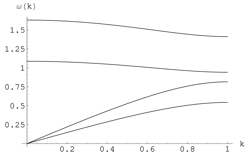
and in Fig. 15 (the vibrational mode broadenings).

Maximal frequencies for longitudinal acoustic and optical modes are and correspondingly, i.e. the ratio , i.e., quite close to the neutron scattering experimental data BB95 , DB99 , SK02 . The robust qualitative features of the broadening for the both longitudinal and transverse acoustic branches occur very similar ones, and can be fitted to . This answer is universal for the model, when the broadening is determined by only one three wave interaction constant .
References
- (1) J.W.Cahn, D.Shechtman, D.Gratias, J.Mat. Res., 1, 13 (1986).
- (2) K.Niizeki, J.Phys. A: Math. Gen., 22, 4295 (1989).
- (3) K.Niizeki, T.Akamatsu, J.Phys.: Cond. Matter., 2, 2759 (1990).
- (4) C.Janot, Quasicrystals: a Primer, Oxford, Oxford Science (1992).
- (5) M. de Boissieu, M.Boudard, R.Bellissent, M.Quilichini, B.Hennion, R.Currat, A.I.Goldman, C.Janot, J.Phys.: Condens. Matter, 5, 4945 (1993).
- (6) J.Hafner, M.Krajci, J.Phys.: Condens. Matter, 5, 2489 (1993).
- (7) M.Boudard, M.de Boissieu, S.Kycia, A.I.Goldman, B.Hennion, R.Bellissent, M.Quilichini, R.Currat, C.Janot, J.Phys.: Condens. Matter, 7, 7299 (1995).
- (8) C.Janot, Phys. Rev. B, 53, 181 (1996).
- (9) P.A.Kalugin, M.A.Chernikov, A.Bianchi, H.R.Ott, Phys. Rev. B., 53, 1445 (1996).
- (10) M.Quilichini, T.Janssen, Rev. Mod. Phys., 69, 277 (1997).
- (11) M.A.Chernikov, H.R.Ott, A.Bianchi, A.Migliori, T.W.Darling, Phys. Rev. Lett., 80, 321 (1998).
- (12) R.Bellissent, M. de Boissieu, G.Coddens in Physical properties of quasicrystals, Z.M. Stadnik, ed., Springer (1999).
- (13) F.Dugain, M.de Boissieu, K.Shibata, R.Currat, T.J.Sato, A.R.Kortan, J.B.Suck, K.Hradil, F.Frey, A.P.Tsai, Eur. Phys. J. B, 7, 513 (1999).
- (14) T.Janssen, Ferroelectrics, 236, 157 (2000).
- (15) K.Gianno, A.V. Sologubenko, M.A.Chernikov, H.R.Ott, Phys. Rev. B, 62, 292 (2000).
- (16) K.Shibata, R.Currat, M. de Boissieu, T.J.Sato, H.Takakura, A.P.Tsai, J.Phys.: Condens. Matter, 14, 1847 (2002).
- (17) C.A.Swenson, I.R.Fisher, N.E.Anderson, Jr., P.C.Canfield, A.Migliori, Phys. Rev. B, 65, 184206 (2002).
- (18) C.A.Swenson, T.A.Lograsso, A.R.Ross, N.E.Anderson, Jr., Phys. Rev. B, 66, 184206 (2002).
- (19) M.Kleman, Eur. Phys. J., B, 31, 315 (2003).
- (20) V.V.Savkin, A.N.Rubtsov, T.Janssen, 31, 525 (2003).
- (21) E.Courtens, M.Foret, B.Hehlen, B.Rufflé, R.Vacher, J.Phys.: Condens. Mattter, 15, 1281 (2003).
- (22) B.Rufflé, M.Foret, E.Courtens, R.Vacher, G.Monaco, Phys. Rev. Lett., 90, 095502 (2003).
- (23) J.P.Lu, T.Odugaki, J.L.Birman, Phys. Rev. B, 33, 4809 (1986).
- (24) L.D.Landau, E.M.Lifshits, Physical Kinetics (Course of Theoretical Physics, volume 10), Pergamon Press, New York (1981).
- (25) S.Roche, D.Mayou, Phys. Rev. Lett., 79, 2518 (1997).
- (26) S.Roche, D.Bicout, E.Macia, E.Kats, Phys. Rev. Lett., 91, 228101 (2003).
- (27) P.Kramer, R.Neri, Acta Crys., A, 40, 580 (1984).
- (28) H.J.Weaver, Applications of discrete and continuous Fourier analysis, J.Wiley and Sons, New York (1983).