Densities of states of the Falicov-Kimball model off half filling in infinite dimensions

Abstract

An approximate analytical scheme of the dynamical mean field theory (DMFT) is developed for the description of the electron (ion) lattice systems with Hubbard correlations within the asymmetric Hubbard model where the chemical potentials and electron transfer parameters depend on an electron spin (a sort of ions). Considering a complexity of the problem we test the approximation in the limiting case of the infinite-$U$ spinless Falicov-Kimball model. Despite the fact that the Falicov-Kimball model can be solved exactly within DMFT, the densities of states of localized particles have not been completely investigated off half filling. We use the approximation to obtain the spectra of localized particles for various particle concentrations (chemical potentials) and temperatures. The effect of a phase separation phenomenon on the spectral function is considered.

I Introduction

The Falicov-Kimball model Falicov and Kimball (1969) was introduced to describe the thermodynamics of metal-insulator transitions in compounds that contained both itinerant and localized quasiparticles. The spinless Falicov-Kimball model is the simplest example of an interacting fermionic system that displays numerous phase transitions. Despite its relative simplicity, the analysis of the model is very complex and still a lot of open problems remain. The model can describe many phenomena such as metal-insulator transition, ferromagnetism, antiferromagnetism, phase separations, etc.

In the dynamical mean-field theory Metzner and Vollhardt (1989); Georges et al. (1996) which is exact in infinite dimensions Müller-Hartmann (1989) the Falicov-Kimball model can be solved exactly by calculating the grand canonical potential and the single-particle Green’s function Brandt and Mielsch (1989, 1990, 1991). The thermodynamics of the Falicov-Kimball model is well investigated. The phase transitions between homogeneous phases or phase separations are investigated using the mentioned exact methods Stasyuk and Hera (2003); Freericks et al. (1999) as well as using the effective Hamiltonian at the large-$U$ limit Letfulov (1999) (see Ref. Freericks and Zlatić, 2003 for detailed review of the Falicov-Kimball model).

The problem of an evaluation of the spectral function of localized particles is more complex than the investigation of thermodynamics and the phase transitions. The $f$ spectral function related to the localized particles was calculated at half-filling more than ten years ago Brandt and Urbanek (1992). Recently, the exact scheme has been extended to the case of different particle concentrations Zlatić et al. (2001), but due to computational difficulties the densities of states of localized particles have not been completely investigated off half filling. So, we suggest here an approximate analytical scheme within the dynamical mean-field theory for calculating the $f$ spectral function at different particle concentrations and temperatures.

We consider the asymmetric Hubbard model describing the dynamics of two types of particles (ions, electrons or quasiparticles) as a generalization of the Falicov-Kimball model. The Hamiltonian of the asymmetric Hubbard model in a second quantization has the following form

$$H=-\sum_{i\sigma}\mu_{\sigma}n_{i\sigma}+U\sum_{i}n_{i\uparrow}n_{i\downarrow}+\sum_{ij\sigma}t_{ij}^{\sigma}a_{i\sigma}^{\dagger}a_{j\sigma}^{\phantom{\dagger}}\,,$$ (1)

where $n_{i\sigma}=a_{i\sigma}^{\dagger}a_{i\sigma}^{\phantom{\dagger}}$ and the motion of particles is described by the creation ($a_{i\sigma}^{\dagger}$) and annihilation ($a_{i\sigma}^{\phantom{\dagger}}$) operators. The chemical potentials $\mu_{\sigma}$ and the transfer parameters $t_{ij}^{\sigma}$ depend on a sort of particles (an electron spin). The value $U$ describes the local on-site repulsion.

The asymmetric Hubbard model was proposed for the description of mixed-valence compounds Kocharian and Reich (1994). This model can also be used for the investigation of the lattice systems having an ionic conductivity with two types of ions. When a single lattice site can be occupied only by one ion, the nontrivial limit $U\rightarrow\infty$ should be considered. Is this case, various thermodynamic regimes can be realized. The chemical potentials or concentrations of particles of different sorts can be fixed independently. In this context the model can be investigated in the presence of the external field corresponding to the difference between the chemical potentials of different sorts.

A number of methods for describing the strongly correlated electron systems has been developed within the dynamical mean field theory. However, all these methods have various restrictions. The quantum Monte-Carlo method Jarrell (1992); Rozenberg et al. (1992); Georges and Krauth (1992) is numerically exact but has severe problems at low temperatures and for high repulsion strength $U$. The exact diagonalization method Caffarel and Krauth (1994); Si et al. (1994) is restricted to a small number of orbitals. Among the numerical techniques the most reliable one at low temperatures is the numerical renormalization group method Bulla (2000). For example its extension was used for the description of the ground state of the standard Hubbard model Zitzler et al. (2002).

Besides the numerical approaches the development of analytical approximations for the infinite-dimensional model still remains necessary. The Hubbard model in the large-$U$ limit was investigated using the non-crossing approximation Pruschke et al. (1993); Obermeier et al. (1997). Many approximations were developed for the weak-coupling regime, for example, the Edwards-Hertz approach Edwards and Hertz (1990); Edwards (1993); Wermbter and Czycholl (1994, 1995). The alloy-analogy based approximations Herrmann and Nolting (1996); Potthoff et al. (1998a, b) do not take into account the effect of scattering processes on forming the energy band and cannot be used for the investigation of spectra of the asymmetric Hubbard model. In the Falicov-Kimball limit, the alloy-analogy (AA) and modified alloy-analogy (MAA) approximations give the density of states of localized particles in the form of a delta function. The scattering processes should be taken into account for a correct description of the broadening of this peak. For example, it was the Hubbard-III approximation Hubbard (1964) that originally included the electron scattering for the half-filled Hubbard model into the theory.

We use and improve the approximate analytical approach originally proposed for the Hubbard model Stasyuk (2000) and extended to the asymmetric Hubbard model Stasyuk and Hera (2003). In this method the single-site problem is formulated in terms of the auxiliary Fermi-field. The approach is based on the equations of motion and on the irreducible Green’s function technique with projecting on the basis of Fermi-operators. This approach gives DMFT equations in the approximation which is a generalization of Hubbard-III approximation and includes as simple specific cases the AA and MAA approximations.

The approximation is tested on the infinite-$U$ spinless Falicov-Kimball model. We use the approximation to obtain the densities of states of localized particles for various chemical potentials (concentrations) and temperatures. The dependences of the chemical potentials on the particle concentrations are calculated using the densities of states as well as thermodynamically by calculating the grand canonical potential Stasyuk and Shvaika (2002). To calculate the particle spectra at low temperatures the phase separation should be taken into account.

In Section II, we review the formalism of DMFT with the use of the auxiliary Fermi-field and the approximate analytical scheme based on the projecting technique and the different-time decoupling procedure. In Section III and in Appendix, the exact relations between some Green’s functions are derived, which allows us to find the projecting coefficients using only the single particle Green’s function and the coherent potential. The results are discussed in Section IV, followed by our conclusions in Section V.

II Formalism

In the dynamical mean-field theory the infinite-dimensional lattice model is mapped on the single-site problem

$${}\mathrm{e}^{-\beta H}\rightarrow\mathrm{e}^{-\beta H_{\mathrm{eff}}}=\mathrm{e}^{-\beta H_{0}}$$

$${}\times\mathcal{T}\exp\Bigg{[}-\int_{0}^{\beta}\!\!\mathrm{d}\tau\!\!\int_{0}^{\beta}\!\!\mathrm{d}\tau^{\prime}\!\sum_{\sigma}J_{\sigma}(\tau-\tau^{\prime})a_{\sigma}^{\dagger}(\tau)a_{\sigma}^{\phantom{\dagger}}(\tau^{\prime})\Bigg{]}$$ (2)

with the coherent potential $J_{\sigma}(\tau-\tau^{\prime})$ which has to be self-consistently determined from the conditions

$$G_{\sigma}(\omega_{n})=\frac{1}{\Xi_{\sigma}^{-1}(\omega_{n})-J_{\sigma}(\omega_{n})},$$ (3)

$$G_{\sigma}(\omega_{n},\mathbf{k})=\frac{1}{\Xi_{\sigma}^{-1}(\omega_{n})-t^{\sigma}_{\mathbf{k}}},$$ (4)

$$G_{\sigma}(\omega_{n})=G_{ii}^{\sigma}(\omega_{n})=\frac{1}{N}\sum_{\mathbf{k}}G^{\sigma}(\omega_{n},\mathbf{k}),$$ (5)

where $G_{\sigma}$ is the one-particle Green’s function, $\Xi_{\sigma}$ is the total irreducible part which does not depend on the wave vector $\mathbf{k}$. The sum over $\mathbf{k}$ in Eq. 5 is calculated by the integration with the density of states (DOS) (a Gaussian DOS for an infinite-dimensional hypercubic lattice and a semielliptic DOS for a $d=\infty$ Bethe lattice).

It was shown in Ref. Stasyuk, 2000 that the single-site problem can be formulated in terms of the auxiliary Fermi-operators $\xi_{\sigma}$ describing the creation and the annihilation of particles in the effective environment. The problem is described by the following Hamiltonian

$$H_{\mathrm{eff}}=H_{0}+\sum_{\sigma}V_{\sigma}\Big{(}a_{\sigma}^{\dagger}\xi_{\sigma}^{\phantom{\dagger}}\!+\xi_{\sigma}^{\dagger}a_{\sigma}^{\phantom{\dagger}}\!\Big{)}+H_{\xi}.$$ (6)

The approach does not require an explicit form of the environment Hamiltonian $H_{\xi}$. The environment is described by the coherent potential given as the Green’s function for the auxiliary Fermi-field with the unperturbed Hamiltonian $H_{\xi}$:

$$J_{\sigma}(\omega)=2\pi V^{2}_{\sigma}\langle\langle\xi_{\sigma}^{\phantom{\dagger}}|\xi_{\sigma}^{\dagger}\rangle\rangle_{\omega}^{\xi}.$$ (7)

The particle creation and annihilation operators are expressed in terms of Hubbard operators

$$a_{\sigma}=X^{0\sigma}+\zeta X^{\bar{\sigma}2}$$ (8)

on the basis of single-site states $|n_{A},n_{B}\rangle$

$$\begin{array}[]{lll}|0\rangle=|0,0\rangle,&&\qquad|A\rangle=|1,0\rangle,\\ |2\rangle=|1,1\rangle,&&\qquad|B\rangle=|0,1\rangle,\end{array}$$ (9)

where the following notations for sort indices are used: $\bar{\sigma}=B$, $\zeta=+$ for $\sigma=A$ and $\bar{\sigma}=A$, $\zeta=-$ for $\sigma=B$. In this representation the local Hamiltonian $H_{0}$ of the asymmetric Hubbard model is

$$H_{0}=-\sum_{\sigma}\big{[}\mu_{\sigma}\big{(}X^{\sigma\sigma}+X^{22}\big{)}\big{]}+UX^{22}\,,$$ (10)

and the two-time Green’s function $G_{\sigma}(\omega)\equiv 2\pi\langle\langle a_{\sigma}^{\phantom{\dagger}}|a_{\sigma}^{\dagger}\rangle\rangle_{\omega}$ is written as:

$$G_{\sigma} = 2\pi\big{[}\langle\langle X^{0\sigma}|X^{\sigma 0}\rangle\rangle_{\omega}+\zeta\langle\langle X^{0\sigma}|X^{2\bar{\sigma}}\rangle\rangle_{\omega}$$ (11)

$${}+\zeta\langle\langle X^{\bar{\sigma}2}|X^{\sigma 0}\rangle\rangle_{\omega}+\langle\langle X^{\bar{\sigma}2}|X^{2\bar{\sigma}}\rangle\rangle_{\omega}\big{]}\,.$$

The Green’s functions in Eq. 11 are calculated using the equations of motion for Hubbard operators:

$$\mathrm{i}\frac{\mathrm{d}}{\mathrm{d}t}X^{0\sigma(\bar{\sigma}2)}(t)=\big{[}X^{0\sigma(\bar{\sigma}2)}\,,H_{\mathrm{eff}}\big{]}\,.$$ (12)

The commutators (12) are projected on the subspace formed by operators $X^{0\sigma}$ and $X^{\bar{\sigma}2}$:

$$\big{[}X^{\gamma},H_{\mathrm{eff}}\big{]}=\alpha_{1}^{\gamma}X^{0\sigma}+\alpha_{2}^{\gamma}X^{\bar{\sigma}2}+Z^{\gamma}\,.$$ (13)

The operators $Z^{0\sigma(\bar{\sigma}2)}$ are defined as orthogonal to the operators from the basic subspace Stasyuk (2000); Stasyuk and Shvaika (2002); Stasyuk and Hera (2003):

$$\langle\{Z^{0\sigma(\bar{\sigma}2)},X^{0\sigma(\bar{\sigma}2)}\}\rangle=0.$$ (14)

These equations determine the projecting coefficients $\alpha_{i}^{0\sigma(\bar{\sigma}2)}$ which are expressed in terms of the mean value

$$\varphi_{\sigma}=\langle\xi_{\bar{\sigma}}^{\phantom{\dagger}}X^{\bar{\sigma}0}\rangle+\zeta\langle X^{\sigma 2}\xi_{\bar{\sigma}}^{\dagger}\rangle.$$ (15)

Using this procedure by differentiating both with respect to the left and to the right time arguments, we come to the relations between the components of the Green’s function $G_{\sigma}$ and scattering matrix $\hat{P}_{\sigma}$. In a matrix representation, we have

$$\hat{G}_{\sigma}=\hat{G}_{0}^{\sigma}+\hat{G}_{0}^{\sigma}\hat{P}_{\sigma}\hat{G}_{0}^{\sigma},$$ (16)

where

$$\hat{G}_{\sigma}=2\pi\left(\begin{array}[]{lll}\langle\langle X^{0\sigma}|X^{\sigma 0}\rangle\rangle&&\langle\langle X^{0\sigma}|X^{2\bar{\sigma}}\rangle\rangle\\ \langle\langle X^{\bar{\sigma}2}|X^{\sigma 0}\rangle\rangle&&\langle\langle X^{\bar{\sigma}2}|X^{2\bar{\sigma}}\rangle\rangle\end{array}\right),$$ (17)

and nonperturbed Green’s function $\hat{G}^{\sigma}_{0}$ is

$$\hat{G}^{\sigma}_{0}=\frac{1}{D_{\sigma}}\left(\begin{array}[]{ccc}\omega-b_{\sigma}&&-\zeta\frac{V_{\sigma}}{A_{2\bar{\sigma}}}\varphi_{\sigma}\\ -\zeta\frac{V_{\sigma}}{A_{0\sigma}}\varphi_{\sigma}&&\omega-a_{\sigma}\end{array}\right)\left(\begin{array}[]{ccc}A_{0\sigma}&&0\\ 0&&A_{2\bar{\sigma}}\end{array}\right),$$ (18)

where

$$A_{pq}=\langle X^{pp}+X^{qq}\rangle,\,\,A_{0\sigma}=1-n_{\bar{\sigma}},\,\,A_{2\bar{\sigma}}=n_{\bar{\sigma}},$$ (19)

$$D_{\sigma}=(\omega-a_{\sigma})(\omega-b_{\sigma})-\frac{V^{2}_{\sigma}}{A_{0\sigma}A_{2\bar{\sigma}}}\varphi_{\sigma}^{2},$$ (20)

$$a_{\sigma}=-\mu_{\sigma}+\frac{V_{\sigma}}{A_{0\sigma}}\varphi_{\sigma},\quad b_{\sigma}=U-\mu_{\sigma}+\frac{V_{\sigma}}{A_{2\bar{\sigma}}}\varphi_{\sigma}.$$ (21)

The scattering matrix

$${}\hat{P}_{\sigma}=2\pi\left(\begin{array}[]{ccc}A_{0\sigma}^{-1}&&0\\ 0&&A_{2\bar{\sigma}}^{-1}\end{array}\right)$$ (24)

$${}\times\left(\begin{array}[]{ccc}\langle\langle Z^{0\sigma}|Z^{\sigma 0}\rangle\rangle&&\langle\langle Z^{0\sigma}|Z^{2\bar{\sigma}}\rangle\rangle\\ \langle\langle Z^{\bar{\sigma}2}|Z^{\sigma 0}\rangle\rangle&&\langle\langle Z^{\bar{\sigma}2}|Z^{2\bar{\sigma}}\rangle\rangle\end{array}\right)\left(\begin{array}[]{ccc}A_{0\sigma}^{-1}&&0\\ 0&&A_{2\bar{\sigma}}^{-1}\end{array}\right)$$ (29)

being expressed in terms of irreducible Green’s functions contains the scattering corrections of the second and the higher orders in powers of $V_{\sigma}$. The separation of the irreducible parts in $\hat{P}_{\sigma}$ enables us to obtain the mass operator $\hat{M}_{\sigma}=\hat{P}_{\sigma}|_{\mathrm{ir}}$ and the single-site Green’s function expressed as a solution of the Dyson equation

$$\hat{G}_{\sigma}=(1-\hat{G}^{\sigma}_{0}\hat{M}_{\sigma})^{-1}\hat{G}^{\sigma}_{0}.$$ (30)

We restrict ourselves to the simple approximation in calculating the mass operator $\hat{P}_{\sigma}$, taking into account the scattering processes of the second order in $V_{\sigma}$. In this case

$$\hat{M}_{\sigma}=\hat{P}_{\sigma}^{(0)},$$ (31)

where the irreducible Green’s functions are calculated without allowance for correlation between electron transition on the given site and environment. It corresponds to the procedure of different-time decoupling, which means in our case an independent averaging of the products of $X$ and $\xi$ operators.

Let us illustrate this approximation on the example of calculation of the following irreducible Green’s function:

$$I(\omega)\equiv\langle\langle{(X^{00}+X^{\sigma\sigma})\xi_{\sigma}^{\phantom{\dagger}}}|{\xi_{\sigma}^{\dagger}(X^{00}+X^{\sigma\sigma})}\rangle\rangle_{\omega}^{\mathrm{ir}}\,.$$ (32)

According to the spectral theorem, this Green’s function is related to the corresponding time correlation function, and according to the different-time decoupling we have

$${}\langle\xi_{\sigma}^{\dagger}(t)(X^{00}+X^{\sigma\sigma})_{t}(X^{00}+X^{\sigma\sigma})\xi_{\sigma}^{\phantom{\dagger}}\rangle^{\mathrm{ir}}$$

$${\qquad}\approx\langle(X^{00}+X^{\sigma\sigma})_{t}(X^{00}+X^{\sigma\sigma})\rangle\langle\xi_{\sigma}^{\dagger}(t)\xi_{\sigma}^{\phantom{\dagger}}\rangle.$$ (33)

Calculation of these correlation functions in a zero approximation

$${}\langle(X^{00}+X^{\sigma\sigma})_{t}(X^{00}+X^{\sigma\sigma})\rangle$$

$${\qquad}\approx\langle(X^{00}+X^{\sigma\sigma})^{2}\rangle=A_{0\sigma}$$ (34)

leads to the result

$$I(\omega)=A_{0\sigma}\langle\langle\xi_{\sigma}^{\phantom{\dagger}}|\xi_{\sigma}^{\dagger}\rangle\rangle_{\omega}^{\xi}=\frac{A_{0\sigma}}{2\pi V^{2}}J_{\sigma}(\omega).$$ (35)

Using the above procedure we can obtain the final expressions for the mass operator and the total irreducible part:

$$\Xi_{\sigma}^{-1}(\omega) = \bigg{[}\frac{A_{0\sigma}}{\omega+\mu_{\sigma}-\tilde{\Omega}_{\sigma}(\omega)}+\frac{A_{2\bar{\sigma}}}{\omega+\mu_{\sigma}-U-\tilde{\Omega}_{\sigma}(\omega)}\bigg{]}^{-1}$$ (36)

$${}+\tilde{\Omega}_{\sigma}(\omega),$$

where

$$\tilde{\Omega}_{\sigma}(\omega)=J_{\sigma}(\omega)-\frac{R_{\sigma}(\omega)}{A_{0\sigma}A_{2\bar{\sigma}}}+\frac{V_{\sigma}\varphi_{\sigma}(\omega)}{A_{0\sigma}A_{2\bar{\sigma}}},$$ (37)

and

$${R_{\sigma}(\omega)=-\frac{\langle X^{\sigma\sigma}+X^{\bar{\sigma}\bar{\sigma}}\rangle}{2}J_{\bar{\sigma}}(\omega+\mu_{\sigma}-\mu_{\bar{\sigma}})}$$

$$-\frac{\langle X^{\sigma\sigma}-X^{\bar{\sigma}\bar{\sigma}}\rangle}{2\pi}\!\int\limits_{-\infty}^{+\infty}\!\frac{\mathrm{d}\omega^{\prime}\,\mathrm{Im}\,J_{\bar{\sigma}}(\omega^{\prime}+\mathrm{i}\varepsilon)}{\omega-\omega^{\prime}-\mu_{\bar{\sigma}}+\mu_{\sigma}}\tanh\frac{\beta\omega^{\prime}}{2}$$

$$+\frac{\langle X^{00}+X^{22}\rangle}{2}J_{\bar{\sigma}}(U-\mu_{\sigma}-\mu_{\bar{\sigma}}-\omega)$$

$${-}\frac{\langle X^{00}-X^{22}\rangle}{2\pi}\!\int\limits_{-\infty}^{+\infty}\!\!\frac{\mathrm{d}\omega^{\prime}\,\mathrm{Im}\,J_{\bar{\sigma}}(-\omega^{\prime}-\mathrm{i}\varepsilon)}{\omega-\omega^{\prime}+\mu_{\bar{\sigma}}+\mu_{\sigma}-U}\tanh\frac{\beta\omega^{\prime}}{2}.$$ (38)

The approach used here for the approximate solution of the single-site problem can be called as the generalized Hubbard-III (GH3) approximation. It becomes the standard Hubbard-III approximation in the case of the usual Hubbard model at half-filling with spin degeneration ($n_{\uparrow}=n_{\downarrow}=1/2$, $\mu_{\uparrow}=\mu_{\downarrow}=U/2$, $\langle X^{00}\rangle=\langle X^{22}\rangle$, $\langle X^{\sigma\sigma}\rangle=\langle X^{\bar{\sigma}\bar{\sigma}}\rangle$):

$$\Xi_{\sigma}^{-1}(\omega) = \bigg{[}\frac{1/2}{\omega+U/2-3J_{\sigma}(\omega)}+\frac{1/2}{\omega-U/2-3J_{\sigma}(\omega)}\bigg{]}^{-1}$$ (39)

$${}+3J_{\sigma}(\omega).$$

The function $R_{\sigma}(\omega)$ describes band forming for particles of sort $\sigma$ by the motion of particles of another sort $\bar{\sigma}$ (scattering processes). The neglect of this contribution ($R_{\sigma}(\omega)=0$) gives MAA approximation. If we put $R_{\sigma}(\omega)=0$ and $\varphi_{\sigma}=0$, the system is described within the simple AA approximation.

In the limit of infinite repulsion $U$ the following solution of the single-site problem is obtained Stasyuk and Hera (2003):

$$G_{\sigma}(\omega)=\frac{1-n_{\bar{\sigma}}}{\omega+\mu_{\sigma}-\frac{V_{\sigma}\varphi_{\sigma}}{1-n_{\bar{\sigma}}}-J_{\sigma}(\omega)+\frac{R_{\sigma}(\omega)}{1-n_{\bar{\sigma}}}}\,,$$ (40)

$$R_{\sigma}(\omega)=-\frac{n_{\sigma}+n_{\bar{\sigma}}}{2}J_{\bar{\sigma}}(\omega+\mu_{\sigma}-\mu_{\bar{\sigma}})$$ (41)

$$-\frac{n_{\sigma}-n_{\bar{\sigma}}}{2\pi}\int\limits_{-\infty}^{+\infty}\frac{\,\mathrm{Im}\,J_{\bar{\sigma}}(\omega^{\prime}+\mathrm{i}\varepsilon)\mathrm{d}\omega^{\prime}}{\omega-\omega^{\prime}-\mu_{\bar{\sigma}}+\mu_{\sigma}}\tanh\frac{\beta\omega^{\prime}}{2}\,.$$

The constant ${\varphi_{\sigma}=\langle\xi_{\bar{\sigma}}^{\phantom{\dagger}}X^{\bar{\sigma}0}\rangle+\zeta\langle X^{\sigma 2}\xi_{\bar{\sigma}}^{\dagger}\rangle}$ can be calculated using the exact relation given in the next section. The average particle concentrations are calculated using the imaginary part of the Green’s functions (density of states):

$$\rho_{\sigma}(\omega)=-\frac{1}{\pi}\,\mathrm{Im}\,G_{\sigma}(\omega+\mathrm{i}\varepsilon).$$ (42)

The self-consistency conditions (a set of equations (3) – (5)) relate the coherent potential $J_{\sigma}$ to the Green’s function $G_{\sigma}$. For the Bethe lattice with a semielliptic density of states

$$\rho^{\mathrm{Bethe}}_{\sigma}(\varepsilon)=\frac{2}{\pi W_{\sigma}^{2}}\sqrt{W_{\sigma}^{2}-\varepsilon^{2}}\,,\quad|\varepsilon|<W_{\sigma}$$ (43)

we have

$$J_{\sigma}(\omega)=\frac{W_{\sigma}^{2}}{4}\,G_{\sigma}(\omega).$$ (44)

In the case of the Falicov-Kimball model the unperturbed bandwidth is zero ($2W_{B}=0$, $J_{B}(\omega)=0$) for localized particles, and the approach gives the exact equation for the Green’s function of itinerant particles $G_{A}(\omega)$. The density of state $\rho_{A}(\omega)$ on the Bethe lattice is nonzero for ${|\omega+\mu_{A}|<W_{A}\sqrt{1-n_{B}}}$:

$$\rho_{A}(\omega)=\frac{2}{\pi W_{A}^{2}}\sqrt{W_{A}^{2}(1-n_{B})-(\omega+\mu_{A})^{2}}.$$ (45)

In this case the equations (40), (41) give an explicit approximate expression for the Green’s function of localized particles:

$$G_{B}(\omega)=\frac{1-n_{A}}{\omega+\mu_{B}-\frac{V_{B}\varphi_{B}}{1-n_{A}}+\frac{R_{B}(\omega)}{1-n_{A}}}\,,$$ (46)

where

$$R_{B}(\omega)=-\frac{n_{B}+n_{A}}{2}J_{A}(\omega+\mu_{B}-\mu_{A})$$ (47)

$$-\frac{n_{B}-n_{A}}{2\pi}\int\limits_{-\infty}^{+\infty}\frac{\,\mathrm{Im}\,J_{A}(\omega^{\prime}+\mathrm{i}\varepsilon)\mathrm{d}\omega^{\prime}}{\omega-\omega^{\prime}-\mu_{A}+\mu_{B}}\tanh\frac{\beta\omega^{\prime}}{2}\,.$$

III The projecting coefficients in equations of motion for Hubbard operators

The average values $\langle X^{pq}\xi_{\sigma}\rangle$ are calculated using corresponding Green’s functions according to the spectral theorem

$$\langle X^{pq}\xi_{\sigma}^{\phantom{\dagger}}\rangle=\int\limits_{-\infty}^{+\infty}{\frac{\mathrm{d}\omega}{\mathrm{e}^{\beta\omega}+1}}\Big{[}-2\,\mathrm{Im}\,\langle\langle\xi_{\sigma}^{\phantom{\dagger}}|X^{pq}\rangle\rangle_{\omega+\mathrm{i}\varepsilon}\Big{]}.$$ (48)

These Green’s functions can be calculated using the exact relation (59) derived in Appendix

$$V_{\sigma}\langle\langle\xi_{\sigma}^{\phantom{\dagger}}|X^{pq}\rangle\rangle_{\omega}=J_{\sigma}(\omega)\langle\langle a_{\sigma}|X^{pq}\rangle\rangle_{\omega}.$$ (49)

For the asymmetric Hubbard model we have to calculate the coefficients $V_{\sigma}\varphi_{\sigma}$:

$$\varphi_{\sigma}=\langle\xi_{\bar{\sigma}}X^{\bar{\sigma}0}\rangle+\zeta\langle X^{\sigma 2}\xi_{\bar{\sigma}}^{\dagger}\rangle=\langle\xi_{\bar{\sigma}}(X^{\bar{\sigma}0}+\zeta X^{2\sigma})\rangle$$ (50)

which are expressed as

$$V_{\sigma}\varphi_{\sigma}=\int_{-\infty}^{+\infty}\frac{\mathrm{d}\omega}{\mathrm{e}^{\beta\omega}+1}\,\mathrm{Im}\,\rho_{\sigma}^{\varphi}(\omega+\mathrm{i}\varepsilon)\,,$$ (51)

$$\rho_{\sigma}^{\varphi}(\omega) = 2J_{\bar{\sigma}}(\omega)\langle\langle X^{0\bar{\sigma}}-\zeta X^{\sigma 2}|X^{\bar{\sigma}0}+\zeta X^{2\sigma}\rangle\rangle_{\omega}$$ (52)

$$= 2J_{\bar{\sigma}}(\omega)\big{[}\langle\langle X^{0\bar{\sigma}}|X^{\bar{\sigma}0}\rangle\rangle_{\omega}-\langle\langle X^{{\sigma}2}|X^{2{\sigma}}\rangle\rangle_{\omega}\big{]}.$$

In the limit of infinite on-site repulsion $U$ the state with double occupation is excluded and we have

$$\rho_{\sigma}^{\varphi}(\omega)=\frac{1}{\pi}J_{\bar{\sigma}}(\omega)G_{\bar{\sigma}}(\omega)\,.$$ (53)

For the Falicov-Kimball model it is possible to calculate the exact Green’s functions for itinerant particles and it gives the exact expression for $V_{B}\varphi_{B}$.

Let us note that previously this parameter was calculated approximately using the Green’s functions obtained by means of the linearized equations of motion and neglecting the irreducible parts Stasyuk (2000); Stasyuk and Shvaika (2002); Stasyuk and Hera (2003). In the model with infinite $U$ this approximate value is

$$\rho_{B}^{\varphi}(\omega)=\frac{1}{\pi}J_{A}(\omega)\frac{1-n_{B}}{\omega+\mu_{B}}\,,$$ (54)

and it corresponds to the approximation of the series (65) where only the first term (the zero approximation for $G_{A}$) is taken into account.

There is shown a comparison between the approximate and the exact values of $\varphi_{B}$ in Fig. 1. The improvement given by the exact relation (53) allows us to investigate the system at low temperatures where summing up the whole series (65) is essential.

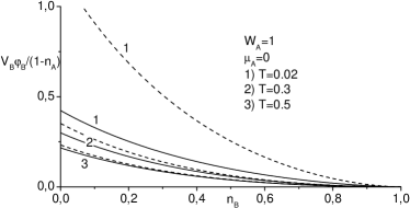
Figure 1: The exact values of $\varphi$ (solid lines) are compared with the approximate ones calculated using the relation (54) (dashed lines) for various temperatures and $n_{B}$. One can see that the approximation is applicable only for very high temperatures.

IV Results

Dependences of chemical potentials $\mu_{A}$ and $\mu_{B}$ on the particle concentrations are calculated using corresponding densities of states. DOS of localized particles is obtained as an imaginary part of the Green’s function

$$\rho_{B}(\omega)=-\frac{1}{\pi}\,\mathrm{Im}\,G_{B}(\omega+\mathrm{i}\varepsilon)\,.$$ (55)

This Green’s function has the correct analytic properties (relations between imaginary and real parts) within the considered approximations (GH3, MAA, AA). The approximate DOS always has the correct sign and the sum rule is fulfilled: the integral of DOS over all frequency is equal to unity for finite $U$ and is equal to $1-n_{\bar{\sigma}}$ for $U\rightarrow\infty$ when the upper band tends to infinity.

Figure 2: DOS of localized particles for the Falicov-Kimball model on the hypercubic lattice with noninteracting DOS $\rho_{A}^{\mathrm{hyp}}(\varepsilon)=\pi^{-1/2}\exp(-\varepsilon^{2})$ at half-filling ($n_{A}=n_{B}=1/2$). Solid line – our approximation; dashed line – exact result Brandt and Urbanek (1992).

For the Falicov-Kimball model the density of states of localized particles can be calculated exactly Brandt and Urbanek (1992); Zlatić et al. (2001); Freericks and Zlatić (2003), but numerical results were obtained mostly at half-filling. The constant $\varphi_{B}$ is zero at half-filling ($n_{A}=n_{B}=1/2$) because of the particle-hole symmetry. In this case we have the simple approximate solution of the single-site problem

$$G_{B}(\omega)=\frac{\omega-2J_{A}(\omega)}{\omega^{2}-U^{2}/4-2\omega J_{A}(\omega)}.$$ (56)

This result at half-filling is independent of temperature, but for high temperatures and large values of $U$ the approximate scheme reproduces the exact results (Fig. 2).

For simplicity we restrict our investigation to the Falicov-Kimball model with the infinite repulsion $U$ on the Bethe lattice. In this case the model describes the system with an average site occupation no more than unity. There is a homogeneous state for temperatures larger than critical $T_{\mathrm{c}}\approx 0.060W_{A}$. For lower temperatures ($T<T_{\mathrm{c}}$) there are various types of phase transitions depending on a thermodynamic regime Freericks et al. (1999); Letfulov (1999); Stasyuk and Hera (2003).

First, we consider a possibility of describing the phase transitions using the approximate equations. For this reason, the behavior of dependences of the chemical potential $\mu_{B}$ on the concentration of localized particles $n_{B}$ is investigated. The phase transition is indicated by the thermodynamic unstable region where $\partial\mu_{B}/\partial n_{B}<0$. When the critical temperature is approached from below, the dependence $\mu_{B}(n_{B})$ becomes monotonic ($\partial\mu_{B}/\partial n_{B}\geq 0$).

Figure 3: The dependence of $\mu_{B}$ on $n_{B}$ in different approximations is compared with the exact result obtained thermodynamically. The parameter values: $W_{A}=1$, $W_{B}=0$, $U=\infty$. 1 – exact result; 2 – MAA; 3 – GH3.

Figure 4: DOS of localized particles within the GH3 approximation for various $\mu_{A}$ and temperatures. $W_{A}=1$; $W_{B}=0$; $U=\infty$; 1) $T=0.06$, 2) $T=0.2$.

In Fig. 3 the approximate curves $\mu_{B}(n_{B})$ are compared with the exact results obtained thermodynamically Stasyuk and Shvaika (2002); Stasyuk and Hera (2003). The alloy-analogy based approximations give the density of states of localized particles in a form of a noninteracting delta-function, which is correct in the atomic limit ${t_{A}=0}$. Thus, the MAA approximation can give reasonable results only when the chemical potential $\mu_{A}<0$ (i.e. the concentration of itinerant particles tends to zero). This approximation shows the presence of a phase transition. However, it overestimates the critical temperature. In Fig. 3 the exact curve at $T=0.060$ is already monotonic but the MAA approximation shows the region with unstable concentration values, i.e. there is still a phase transition.

The GH3 approximation, unlike the MAA approximation, incorporates the scattering processes forming the energy band of localized particles. This is crucial for the calculation of thermodynamic quantities. The approximate curves coincide with the exact ones in a wide range of temperatures for the concentrations larger than some value which depends on $\mu_{A}$. In Fig. 3 ($\mu_{A}=0$) one can see a good agreement with the exact result at $\mu_{A}=0$ for concentrations $n_{B}\gtrsim 0.5$. At temperatures lower than the critical one the approximation clearly indicates the phase transition and gives the correct value for $T_{\mathrm{c}}\backsimeq 0.060$.

Spectra of localized particles are plotted in Fig. 4. In this case temperatures are higher than the critical one, so a homogeneous state is stable. The parameter values are chosen so that the approximation gives the correct thermodynamic $\mu_{B}(n_{B})$ relations. The energy band of itinerant particles (A) depends only on a concentration $n_{B}$ and its width is $2W_{A}\sqrt{1-n_{B}}$. However, the band of localized particles (B) is generated by scattering processes and its spectral shape depends on the concentration $n_{B}$, the chemical potential $\mu_{A}$ (or the corresponding concentration $n_{A}$) and temperature.

Depending on the values of the chemical potential of itinerant particles $\mu_{A}$ (or $n_{A}$) there are two limiting cases with different properties of the localized particle spectrum. For very small $n_{A}$ (negative $\mu_{A}$) the system is close by its behavior to the atomic limit, i.e., the spectrum $\rho_{B}(\omega)$ is in the form of a delta peak. The sharp peak is slightly broadened by the scattering of itinerant particles (Fig. 4A, $\mu_{A}=-0.4$). The contrary case with the nearly filled bands is when the total concentration of particles tends to unity, $n_{A}+n_{B}\rightarrow 1$ (Fig. 4C, $\mu_{A}=0.4$). In this case the peak vanishes because the contribution of the coherent potential of mobile particles $J_{A}(\omega)$ and the corresponding function $R_{B}(\omega)$ (47) becomes larger and the simple pole in (46) disappears. The spectrum $\rho_{B}(\omega)$ corresponds by the form to the lower Hubbard subband (or the lower subband for the half-filled Falicov-Kimball model obtained in Ref. Brandt and Urbanek, 1992) with the chemical potential located in a gap in the strong coupling limit. The intermediate case with the broad band superimposed by the sharp peak is shown in Fig. 4B.

Figure 5: DOS of localized particles within the GH3 approximation ($W_{A}=1$, $W_{B}=0$). A) At temperatures below $T_{\mathrm{c}}$ ($T=0.059$) the state is separated into two phases with different particle concentrations (1,2 – the spectra of each component; 3 – the superposition of 1 and 2). B) DOS for various temperatures (1 – $T=0.059$, 2 – $T=0.061$, 3 – $T=0.2$, 4 – $T=1.0$).

States with concentration values in some region (where $\partial\mu_{\sigma}/\partial n_{\sigma}<0$) are thermodynamically unstable at low temperatures. So, the presence of phase transitions should be taken into consideration. There are phase transitions between homogeneous phases with a concentration jump in the thermodynamic regime with the fixed chemical potentials ($\mu_{A}=\mathrm{const}$, $\mu_{B}=\mathrm{const}$). In this case the density of states changes instantly as the concentration jumps. If one of the concentrations ($n_{A}$ or $n_{B}$) is fixed the homogeneous state is unstable and the phase separation takes place. The phase transitions for the Falicov-Kimball model were investigated in many works (see Ref. Freericks and Zlatić, 2003); the regimes mentioned above were investigated for the Falicov-Kimball model using the exact thermodynamic equations in Ref. Stasyuk and Hera, 2003.

Let us consider the thermodynamic regime with fixed values of $\mu_{A}$ and $n_{B}$. In the homogeneous state the spectral function of itinerant particles $\rho_{A}$ depends on $n_{B}$ and $\mu_{A}$ (Eq. 45) and is independent of temperature. However, in the phase separated state the spectrum of the whole system can be considered as a superposition of spectra of each component. The homogeneous state is unstable for the concentration values $n_{B}\in(n_{B1},n_{B2})$ and the system is separated into two different phases with the concentrations of $B$ particles $n_{B1}\approx 0.52$ and $n_{B2}\approx 0.78$ at $T=0.059W_{A}$. The concentrations of the components ($n_{B1}$, $n_{B2}$) depend on temperature Stasyuk and Hera (2003). Thus, the spectra $\rho_{A}$ and $\rho_{B}$ are temperature dependent in the segregated phase. In Fig. 5(A) DOS of localized particles is plotted at temperature $T=0.059W_{A}<T_{\mathrm{c}}$. In Fig. 5(B) the spectrum at various temperatures is compared. The bandwidth is larger in the segregated state than in the homogeneous state ($T>T_{\mathrm{c}}$) and is temperature dependent.

V Conclusions

The approximate analytic approach within DFMT for calculating the single-particle Green’s functions of the asymmetric Hubbard model is developed and improved. This approximation allows one to investigate the model for various concentration values. The method is tested on the Falicov-Kimball model with the infinite on-site repulsion. It is shown that for high enough temperatures or large concentrations of localized particles the approximate approach reproduces exact values of chemical potentials. The approximation can correctly indicate the instability of a homogenous state and the presence of phase transitions.

The generalized Hubbard-III approximation (GH3) partially includes the scattering of particles into the theory and describes the formation of the band of localized particles. In the infinite-$U$ limit the spectrum of localized particles is obtained for various particle concentrations and temperatures. The form of this spectrum continuously changes from a delta peak to the characteristic form of the lower subband of the spectrum in the Hubbad-III approximation when the chemical potential of itinerant particles increases.

*

Appendix A Exact relations between Green’s functions

Let us consider the effective single-site problem in terms of the auxiliary Fermi-field

$$\hat{H}_{\mathrm{eff}}=\hat{H}_{0}+\hat{H}_{\xi}+\sum_{\sigma=1}^{m}V_{\sigma}\Big{(}a_{\sigma}^{\dagger}\xi_{\sigma}^{\phantom{\dagger}}\!+\xi_{\sigma}^{\dagger}a_{\sigma}^{\phantom{\dagger}}\!\Big{)},$$ (57)

$\hat{H}_{0}$ is a single-site Hamiltonian; $\hat{H}_{\xi}$ is an auxiliary environment Hamiltonian. The number $m$ of sorts of itinerant particles can be arbitrary ($m=1,\,2,\,3,\,\ldots$). So, the effective Hamiltonian can describe the Falicov-Kimball model ($m=1$) and the Hubbard model ($m=2$). The algebra of $\xi$ operators is defined by the anticommutation relations

$$\{\xi_{\alpha},\,\xi_{\beta}\}=\{\xi_{\alpha}^{\dagger},\,\xi_{\beta}^{\dagger}\}=0,\quad\{\xi_{\alpha}^{\dagger},\,\xi_{\beta}^{\phantom{\dagger}}\!\}=\delta_{\alpha,\beta}\,.$$ (58)

It can be proved that the following relations take place

$$V_{\sigma}\langle\langle\xi_{\sigma}|\hat{A}\rangle\rangle_{\omega} = J_{\sigma}(\omega)\langle\langle a_{\sigma}|\hat{A}\rangle\rangle_{\omega},$$ (59)

$$2\pi V_{\sigma}^{2}\langle\langle\xi_{\sigma}^{\phantom{\dagger}}|\xi_{\sigma}^{\dagger}\rangle\rangle_{\omega} = J_{\sigma}(\omega)+2\pi J^{2}_{\sigma}(\omega)\langle\langle a_{\sigma}^{\phantom{\dagger}}|a_{\sigma}^{\dagger}\rangle\rangle_{\omega},$$ (60)

where $\hat{A}$ is the arbitrary Fermi-operator that anticommutates with the $\xi$ operators, and $J_{\sigma}(\omega)$ is the Green’s function for the unperturbed Hamiltonian

$$J_{\sigma}(\omega)=2\pi V^{2}_{\sigma}\langle\langle\xi_{\sigma}^{\phantom{\dagger}}|\xi_{\sigma}^{\dagger}\rangle\rangle_{\omega}^{\xi}.$$

Proof. Thermodynamic perturbation theory can be formulated based on the interaction representation for the statistical operator with the use of the $H_{0}+H_{\xi}$ operator as the zero-order Hamiltonian:

$${}\hat{\rho}=\mathrm{e}^{-\beta H_{\mathrm{eff}}}=\mathrm{e}^{-\beta(H_{0}+H_{\xi})}\hat{\sigma}(\beta),$$ (61)

$${}\hat{\sigma}(\beta)=\mathrm{e}^{-\beta(H_{0}+H_{\xi})}\mathcal{T}_{\tau}\exp\bigg{[}-\int_{0}^{\beta}\!\!\mathrm{d}\tau\hat{H}_{\mathrm{int}}(\tau)\bigg{]}.$$ (62)

The part of the interaction Hamiltonian describing one sort ($\sigma$) of particles is separated off:

$$\hat{H}_{\mathrm{int}}=V_{\sigma}\Big{(}a_{\sigma}^{\dagger}\xi_{\sigma}^{\phantom{\dagger}}+\xi_{\sigma}^{\dagger}a_{\sigma}^{\phantom{\dagger}}\Big{)}+\hat{B}_{\sigma}.$$ (63)

The residue $\hat{B}_{\sigma}$ commutates with the operators of the chosen sort $\sigma$: $[\hat{B}_{\sigma},\,\xi_{\sigma}]=[\hat{B}_{\sigma},\,\xi_{\sigma}^{\dagger}]=0$. Thus, at the perturbation expansion the operator $\xi_{\sigma}^{(\dagger)}$ does not have to be paired with the operator $\hat{B}_{\sigma}$. Here we introduce notations for the Green’s functions

$$\begin{array}[]{lll}\mathcal{G}_{\sigma}(\tau-\tau^{\prime})&=&\langle\mathcal{T}_{\tau}\xi_{\sigma}^{\dagger}(\tau)\xi_{\sigma}^{\phantom{\dagger}}(\tau^{\prime})\rangle_{0}\\ G_{\sigma}(\tau-\tau^{\prime})&=&\langle\mathcal{T}_{\tau}a_{\sigma}^{\dagger}(\tau)a_{\sigma}^{\phantom{\dagger}}(\tau^{\prime})\rangle\\ \Phi_{\sigma}(\tau-\tau^{\prime})&=&\langle\mathcal{T}_{\tau}\hat{A}_{\sigma}(\tau)\xi_{\sigma}(\tau^{\prime})\rangle\\ G^{A}_{\sigma}(\tau-\tau^{\prime})&=&\langle\mathcal{T}_{\tau}\hat{A}_{\sigma}(\tau)a_{\sigma}(\tau^{\prime})\rangle\end{array}$$

The perturbation theory expansion of the scattering matrix $\hat{\sigma}(\beta)$ gives the following series for the Green’s function $\Phi_{\sigma}(\tau-\tau^{\prime})$:

$${}\Phi_{\sigma}(\tau-\tau^{\prime})=\frac{V_{\sigma}^{2l+1}}{\langle\sigma(\beta)\rangle_{0}}\sum_{p=0}^{\infty}\frac{(-1)}{(2p+1)!}\sum_{l=0}^{p}\frac{(2p+1)!}{l!(l+1)!(2p-2l)!}\int_{0}^{\beta}\mathrm{d}\tau_{1}\ldots\mathrm{d}\tau_{2p+1}$$

$${}\times\langle\mathcal{T}_{\tau}\hat{A}(\tau)\underline{\xi_{\sigma}(\tau^{\prime})}\big{(}a_{\sigma}^{\dagger}\xi_{\sigma}^{\phantom{\dagger}}\big{)}_{1}\cdots\big{(}a_{\sigma}^{\dagger}\xi_{\sigma}^{\phantom{\dagger}}\big{)}_{l}\big{(}\xi_{\sigma}^{\dagger}a_{\sigma}^{\phantom{\dagger}}\big{)}_{l+1}\cdots\big{(}\xi_{\sigma}^{\dagger}a_{\sigma}^{\phantom{\dagger}}\big{)}_{2l+1}\hat{B}_{\sigma}(\tau_{2l+2})\cdots\hat{B}_{\sigma}(\tau_{2p+1})\rangle_{0}\,.$$ (64)

The averaging of $\mathcal{T}$ products is performed in the zero-order Hamiltonian according to the Wick’s theorem by the consecutive pairing. We start the pairing procedure from the operator $\xi_{\sigma}^{\phantom{\dagger}}(\tau^{\prime})$ and it is performed only with the operators $\xi_{\sigma}^{\dagger}$. After the first pairing we have the following expression:

$${}\Phi_{\sigma}(\tau-\tau^{\prime})=\frac{V_{\sigma}^{2l+1}}{\langle\sigma(\beta)\rangle_{0}}\int_{0}^{\beta}\mathrm{d}\tau^{\prime\prime}\mathcal{G}(\tau^{\prime\prime}-\tau^{\prime})\sum_{p=0}^{\infty}\sum_{l=0}^{p}\frac{1}{l!l!(2p-2l)!}\int_{0}^{\beta}\mathrm{d}\tau_{1}\ldots\mathrm{d}\tau_{2p}$$

$${}\times\langle\mathcal{T}_{\tau}\hat{A}(\tau)a_{\sigma}(\tau^{\prime\prime})\big{(}a_{\sigma}^{\dagger}\xi_{\sigma}^{\phantom{\dagger}}\big{)}_{1}\cdots\big{(}a_{\sigma}^{\dagger}\xi_{\sigma}^{\phantom{\dagger}}\big{)}_{l}\big{(}\xi_{\sigma}^{\dagger}a_{\sigma}^{\phantom{\dagger}}\big{)}_{l+1}\cdots\big{(}\xi_{\sigma}^{\dagger}a_{\sigma}^{\phantom{\dagger}}\big{)}_{2l}\hat{B}_{\sigma}(\tau_{2l+1})\cdots\hat{B}_{\sigma}(\tau_{2p})\rangle_{0}\,.$$ (65)

Summing up the series in (65) gives the Green’s function ${G_{\sigma}^{A}(\tau-\tau^{\prime})}$ and we have

$$\Phi_{\sigma}(\tau-\tau^{\prime})=V_{\sigma}\int_{0}^{\beta}\mathrm{d}\tau^{\prime\prime}G_{\sigma}^{A}(\tau-\tau^{\prime\prime})\mathcal{G}_{\sigma}(\tau^{\prime\prime}-\tau^{\prime})\,,$$ (66)

or in the Matsubara frequency representation:

$$\Phi_{\sigma}(\omega_{n})=V_{\sigma}G_{\sigma}^{A}(\omega_{n})\mathcal{G}_{\sigma}(\omega_{n})\,.$$ (67)

Finally, in order to obtain the expression (59), an analytical continuation of the Green’s functions from the imaginary axis to the real one should be done ($\mathrm{i}\omega_{n}\rightarrow{\omega+\mathrm{i}\varepsilon}$, $G_{\sigma}^{A}(\omega_{n})\rightarrow 2\pi\langle\langle a_{\sigma}|\hat{A}\rangle\rangle_{\omega}$, $\Phi_{\sigma}(\omega_{n})\rightarrow 2\pi V_{\sigma}\langle\langle\xi_{\sigma}|\hat{A}\rangle\rangle_{\omega}$, …). If we put $\hat{A}=\xi_{\sigma}^{\dagger}$, the pairing of the operator $\xi_{\sigma}^{\phantom{\dagger}}(\tau^{\prime})$ with $\xi_{\sigma}^{\dagger}(\tau)$ gives the first term in (60). The second term is obtained using the procedure the same as at deriving the relation (59).

References

Falicov and Kimball (1969)
L. M. Falicov and
J. C. Kimball,
Phys. Rev. Lett. 22,
997 (1969).
Metzner and Vollhardt (1989)
W. Metzner and
D. Vollhardt,
Phys. Rev. Lett. 62,
324 (1989).
Georges et al. (1996)
A. Georges,
G. Kotliar,
W. Krauth, and
M. J. Rozenberg,
Rev. Mod. Phys. 68,
13 (1996).
Müller-Hartmann (1989)
E. Müller-Hartmann,
Z. Phys. B 74,
507 (1989).
Brandt and Mielsch (1989)
U. Brandt and
C. Mielsch,
Z. Phys. B 75,
365 (1989).
Brandt and Mielsch (1990)
U. Brandt and
C. Mielsch,
Z. Phys. B 79,
295 (1990).
Brandt and Mielsch (1991)
U. Brandt and
C. Mielsch,
Z. Phys. B 82,
37 (1991).
Stasyuk and Hera (2003)
I. V. Stasyuk and
O. B. Hera,
Condens. Matter Phys. 6,
127 (2003).
Freericks et al. (1999)
J. K. Freericks,
C. Gruber, and
N. Macris,
Phys. Rev. B 60,
1617 (1999).
Letfulov (1999)
B. M. Letfulov,
Eur. Phys. J. B 11,
423 (1999).
Freericks and Zlatić (2003)
J. K. Freericks
and
V. Zlatić,
Rev. Mod. Phys. 75,
1333 (2003).
Brandt and Urbanek (1992)
U. Brandt and
M. P. Urbanek,
Z. Phys. B 89,
297 (1992).
Zlatić et al. (2001)
V. Zlatić,
J. K. Freericks,
R. Lemański,
and G. Czycholl,
Phil. Mag. B 81,
1443 (2001).
Kocharian and Reich (1994)
A. N. Kocharian
and G. R. Reich,
J. Appl. Phys. 76,
6127 (1994).
Jarrell (1992)
M. Jarrell,
Phys. Rev. Lett. 69,
168 (1992).
Rozenberg et al. (1992)
M. J. Rozenberg,
X. Y. Zhang, and
G. Kotliar,
Phys. Rev. Lett. 69,
1236 (1992).
Georges and Krauth (1992)
A. Georges and
W. Krauth,
Phys. Rev. Lett. 69,
1240 (1992).
Caffarel and Krauth (1994)
M. Caffarel and
W. Krauth,
Phys. Rev. Lett. 72,
1545 (1994).
Si et al. (1994)
Q. Si,
M. J. Rozenberg,
G. Kotliar, and
A. E. Ruckenstein,
Phys. Rev. Lett. 72,
2761 (1994).
Bulla (2000)
R. Bulla, Adv.
Solid State Phys. 40, 169
(2000).
Zitzler et al. (2002)
R. Zitzler,
T. Pruschke, and
R. Bulla,
Eur. Phys. J. B 27,
473 (2002).
Pruschke et al. (1993)
T. Pruschke,
D. L. Cox, and
M. Jarrell,
Phys. Rev. B 47,
3553 (1993).
Obermeier et al. (1997)
T. Obermeier,
T. Pruschke, and
J. Keller,
Phys. Rev. B 56,
R8479 (1997).
Edwards and Hertz (1990)
D. M. Edwards and
J. A. Hertz,
Physica B 163,
527 (1990).
Edwards (1993)
D. M. Edwards,
J. Phys.: Condens. Matter 5,
161 (1993).
Wermbter and Czycholl (1994)
S. Wermbter and
G. Czycholl,
J. Phys.: Condens. Matter 6,
5439 (1994).
Wermbter and Czycholl (1995)
S. Wermbter and
G. Czycholl,
J. Phys.: Condens. Matter 7,
7335 (1995).
Herrmann and Nolting (1996)
T. Herrmann and
W. Nolting,
Phys. Rev. B 53,
10579 (1996).
Potthoff
et al. (1998a)
M. Potthoff,
T. Herrmann,
T. Wegner, and
W. Nolting,
phys. stat. sol. (b) 210,
199 (1998a).
Potthoff
et al. (1998b)
M. Potthoff,
T. Herrmann, and
W. Nolting,
Eur. Phys. J. B 4,
485 (1998b).
Hubbard (1964)
J. Hubbard,
Proc. R. Soc. London, Ser. A
281, 401 (1964).
Stasyuk (2000)
I. V. Stasyuk,
Condens. Matter Phys. 3,
437 (2000).
Stasyuk and Shvaika (2002)
I. V. Stasyuk and
A. M. Shvaika,
Ukr. J. Phys. 47,
975 (2002).