Thermodynamics of Two - Band Superconductors: The Case of MgB₂

Abstract

Thermodynamic properties of the multiband superconductor MgB₂ have often been described using a simple sum of the standard BCS expressions corresponding to $\sigma$- and $\pi$-bands. Although, it is a priori not clear if this approach is working always adequately, in particular in cases of strong interband scattering. Here we compare the often used approach of a sum of two independent bands using BCS-like $\alpha$-model expressions for the specific heat, entropy and free energy to the solution of the full Eliashberg equations. The superconducting energy gaps, the free energy, the entropy and the heat capacity for varying interband scattering rates are calculated within the framework of two-band Eliashberg theory. We obtain good agreement between the phenomenological two-band $\alpha$-model with the Eliashberg results, which delivers for the first time the theoretical verification to use the $\alpha$-model as a useful tool for a reliable analysis of heat capacity data. For the thermodynamic potential and the entropy we demonstrate that only the sum over the contributions of the two bands has physical meaning.

I Introduction

Apart from the high transition temperature of 40 K Nagamatsu , two-band superconductivity was the other unexpected phenomenon in MgB₂ which attracts increasing attention. In fact, at present it appears that MgB₂ is the only superconductor with substantiated theoretical and experimental evidence for two-band superconductivity.

Historically, two-band superconductivity has already been investigated theoretically shortly after the formulation of BCS theory. Suhl, Matthias and Walker Suhl suggested a model for transition metals considering overlapping $s$- and $d$-bands. At the same time, Moskalenko proposed an extension of BCS theory for multiple bands Moskalenko . A review of theoretical treatment of the critical temperature $T_{c}$ of multiband superconductors may be found in Ref.Allen, .

In the early sixties there have been experimental claims for the observation of two-band superconductivity in some transition metals like e.g. V, Nb and Ta Shen ; Radebough and later in oxygen depleted SrTiO₃ Bednorz .

Until now, MgB₂ appears to be first system for which multi-band superconductivity has independently been evidenced by several experimental techniques like, for example, heat capacity, tunneling spectroscopy, Raman spectroscopy, penetration depth measurements, ARPRES, and the analysis of the critical fields PhysicaC . The theoretical justification for two-band superconductivity in MgB₂ has been given from electronic structure calculations Kortus ; Pickett . These find that the Fermi surface contains two quasi-cylindrical sheets corresponding to nearly two-dimensional $\sigma$-bands. A three dimensional network of the Fermi surface is attributed to the $\pi$-bands. It has been demonstrated that the optical bond stretching $E_{\mathrm{2g}}$ phonons couple strongly to the holes at the top of $\sigma$-bands while the three-dimensional $\pi$-electrons couple only weakly to the phonons. The different coupling strengths of the $\sigma$- and $\pi$-bands lead to superconducting gaps different in character and size Liu ; Kong ; Bohnen ; Choi ; Kunc . Using linear response theory it is possible to calculate the electron-phonon coupling (Eliashberg functions) from first principles. The superconducting gaps obtained from Eliashberg theory are in very good agreement with the experiments Golubov ; Choi .

Interband scattering from impurities will complicate this picture because interband scattering leads to a decrease of $T_{\mathrm{c}}$ and finally to a single order parameter Schopohl ; GolMaz ; Golubov ; Brinkman . Interband scattering is weak in MgB₂ mazinimp , but this is not necessarily the case in samples in which Mg has been replaced by Al or B by C (Ref.Agrestini, ; Bouquet, ; Junod, ; Xiang, ; Li, ; Margadonna, ; Papavass, ; Bianconi, ; Pena, ; Postorino, ; Castro, ; Putti, ; Ribeiro, ; Schmidt, ; Papagelis, ; Holanova, ; Gonelli1, ) or which have been exposed to neutron irradiation Wangirra . Such samples exhibit considerably reduced $T_{\mathrm{c}}$, while the two gaps persist even at very low critical temperatures. Recently it was shown that the $T_{\mathrm{c}}$ reduction in MgB₂ due to Al or C doping can be explained mainly as due to a simple effect of band filling PRL2005 ; Ummarino . A similar observation has been made using a phenomenological weak-coupling approachBussmann . Further, the doping independent $\pi$-gap in C-doped MgB₂ can be understood as due to a compensation of band filling and interband scattering effects.

Thermodynamic properties of anisotropic superconductors in the weak coupling regime were extensively studied in the past. In the case of weak anisotropy the BCS model was extended by Pokrovsky Pokrov . It was shown that the specific heat jump at $T_{c}$ is reduced as compared to the isotropic case. For two-band weakly coupled superconductors the specific heat was calculated by several authors Moscal91 ; Palistrant92 ; SodaWada ; Geilikman ; ShenSonPhil ; Kresin73 ; Chi ; Mishonov ; Ramunni ; Nakai ; Kristof ; Watanabe (for a recent review see also Ref. Palistrant, ). The main prediction is that at $T_{c}$ the relative jump in the electronic specific heat, $(C_{SC}-C_{N})/C_{N}$, is reduced as compared to the universal BCS value of 1.43. On the other hand, for an isotropic strongly coupled superconductor the relative specific heat jump is larger than 1.43 (see e.g. the review in Ref. Carbotte, ). The combined effect of strong coupling and multiband anisotropy on the specific heat was studied earlier by the present authors Golubov , where the results of the first principles calculations of the electron-phonon interaction in MgB₂ were used but the effect of interband impurity scattering was not considered. Recently strong-coupling corrections were taken into account in the so-called two-square-well approximation (separable model) Zehet ; Mitr ; Nicol , where the effect of interband scattering on some thermodynamic functions was studied Mitr ; Nicol .

In the present work we formulate a generalized description of the thermodynamics of multiband superconductors taking into account impurity scattering (magnetic and nonmagnetic) in the framework of two-band Eliashberg theory. The results are applied to MgB₂ using the first principles band-structure results for the electronic spectra and electron-phonon interaction Kong by extending our preceding approach Golubov . The superconducting energy gaps, the free energy, the entropy and the heat capacity for varying nonmagnetic interband scattering rates are calculated within the framework of two-band Eliashberg theory. It will be shown that the expression for the thermodynamic potential on the extremal trajectory corresponding to solutions of the Eliashberg equations has the form of the sum of contributions of $\sigma$- and $\pi$-bands, but that only the total thermodynamic potential (the sum of both contributions) has physical meaning.

In a second step, we perform a comparison of the phenomenological two-band $\alpha$-model with the Eliashberg results and apply a fit program developed for the $\alpha$-model to extract the gaps and the Sommerfeld constants from the Eliashberg results. Good agreement of the two band $\alpha$-model with the Eliashberg data is found for the temperature dependence of total heat capacity, the entropy and the free energy and the gaps. There are, however, distinct deviations in the partial contributions to the individual quantities and the Sommerfeld constants obtained from the fits. We conclude that the phenomenological $\alpha$-model approach can be taken as a handy tool to analyze e. g. experimental heat capacity data and the gaps to a satisfying accuracy, however that care must be taken for other quantities.

The paper is organized as follows: In Section II the introduction to the formalism and the method of solution is given, in Section III numerical results for the densities of states (DOS) and various thermodynamic quantities as a function of interband impurity scattering rate are discussed, in Section IV the comparison of the two-band $\alpha$-model with the Eliashberg results is performed. In the Appendix a general expression for the thermodynamic potential of a multiband superconductor with nonmagnetic impurities is derived.

II Free energy and Eliashberg Equations

A general expression for the difference of free energies $\Delta`\Omega=\Omega_{N}-\Omega_{S}$ in the normal (N) and superconducting (S) state for a system with electron-phonon interaction and multiple bands can be obtained in two ways: one has been derived by a straightforward integration over the electron-phonon interaction constants by Golubov et al. Golubov . The derivation of the expression for the thermodynamic potential for the case of nonmagnetic as well magnetic impurities is presented in Appendix A. In terms of Matsubara frequencies the $\Omega$-potential can be written as

$$\Omega = \Omega_{e}^{(0)}+\Omega_{\mathrm{ph}}^{(0)}-2\pi\sum_{i}N_{i}(0)T\sum\limits_{n}\frac{\omega_{n}^{2}(Z_{in}^{2}-1)+\Phi_{in}^{2}}{|\omega_{n}|+\sqrt{\omega_{n}^{2}Z_{in}^{2}+\Phi_{in}^{2}}}+$$

$$+\pi\sum_{i}N_{i}(0)T\sum\limits_{n}\frac{\omega_{n}^{2}Z_{in}(Z_{in}-1)+\Phi_{in}^{2}}{\sqrt{\omega_{n}^{2}Z_{in}^{2}+\Phi_{in}^{2}}},$$

where $\Omega_{e}^{(0)}$ is the $\Omega$-potential of the noninteracting electrons, and $\Omega_{\mathrm{ph}}^{(0)}$ is the $\Omega$-potential of the noninteracting phonons.

For the difference of the $\Omega$-potentials in the normal and the superconducting state one obtains

$$\Delta\Omega = \Omega_{N}-\Omega_{S}=-\pi\sum_{i}N_{i}(0)T\sum\limits_{n=-\omega_{c}}^{\omega_{c}}$$

$$\left\{|\omega_{n}|(Z_{in}^{N}-1)-\frac{2\omega_{n}^{2}[\left(Z_{in}^{S}\right)^{2}-1]+2\Phi_{in}^{2}}{|\omega_{n}|+\sqrt{\omega_{n}^{2}\left(Z_{in}^{S}\right)^{2}+\Phi_{in}^{2}}}+\frac{\omega_{n}^{2}Z_{in}^{S}(Z_{in}^{S}-1)+\Phi_{in}^{2}}{\sqrt{\omega_{n}^{2}\left(Z_{in}^{S}\right)^{2}+\Phi_{in}^{2}}}\right\}.$$

$Z$ is the renormalization factor (which is unity in the weak coupling limit) and $\Phi$ is the order parameter which is connected to the energy gap via $\Delta_{i}(\omega_{n})=\Phi_{i}(\omega_{n})/Z_{i}(\omega_{n})=\Phi_{in}/Z_{in}$. $Z^{N}$ and $Z^{S}$ correspond to the normal state ($\Delta$ = 0) and the superconducting state, respectively. The summations in Eq. II are carried out over the fermionic Matsubara (temperature) frequencies $\omega_{n}=\pi T(2n-1)$ as well as over the band index $i=\sigma,\pi$. $N_{i}(0)$ are the partial electronic DOS’s for the $\sigma$- and $\pi$-bands at the Fermi level.

Another way to express the free energy was suggested by Carbotte Carbotte , who proposed that it is possible to find a functional, which minimization with respect to $Z$ and $\Phi$ gives the Eliashberg relations for superconductors with strong electron-boson interaction. For a multiband system the corresponding functional is given by

$$\Delta\mathcal{F}=2\pi T\sum_{i,n}N_{i}(0)\omega_{n}\left(\frac{Z_{in}\omega_{n}}{\sqrt{\left(Z_{in}\omega_{n}\right)^{2}+\Phi_{in}^{2}}}-\text{sign}\omega_{n}\right)$$

$$+\pi^{2}T^{2}\sum_{n,m}\sum_{i,j}N_{i}(0)\left[\frac{Z_{in}\omega_{n}}{\sqrt{\left(Z_{in}\omega_{n}\right)^{2}+\Phi_{in}^{2}}}\frac{Z_{m,j}\omega_{m}}{\sqrt{\left(Z_{jm}\omega_{m}\right)^{2}+\Phi_{jm}^{2}}}-\text{sign}(\omega_{n}\omega_{m})\right]\tilde{\lambda}_{ij}^{+}(\omega_{n}-\omega_{m})$$

$$+\pi^{2}T^{2}\sum_{n,m}^{|\omega_{c}|}\sum_{i,j}N_{i}(0)\frac{\Phi_{in}}{\sqrt{\left(Z_{in}\omega_{n}\right)^{2}+\Phi_{in}^{2}}}\frac{\Phi_{jm}}{\sqrt{\left(Z_{jm}\omega_{m}\right)^{2}+\Phi_{jm}^{2}}}\left[\tilde{\lambda}_{ij}^{-}(\omega_{n}-\omega_{m})-\mu_{ij}^{\ast}(\omega_{c})\right],$$ (2)

where

$$\tilde{\lambda}_{ij}^{\pm}(\omega_{n}-\omega_{m})=\int_{0}^{\infty}\frac{d\omega^{2}\alpha_{ij}^{2}(\omega)F_{ij}(\omega)}{(\omega_{n}-\omega_{m})^{2}+\omega^{2}}+\left(\Gamma_{ij}\pm\Gamma_{ij}^{m}\right)\delta_{n,m}/2\pi T$$

represents the electron-phonon interaction together with nonmagnetic $\Gamma_{ij}$ and magnetic $\Gamma_{ij}^{m}$ impurity scattering terms. The Coulomb pseudopotential $\mu_{ij}^{\ast}(\omega_{c})$ is determined at a frequency $\omega_{c}$ which has to be chosen much larger than the maximal phonon frequency. Minimization of Eq. 2 provides the Eliashberg equations on the imaginary (Matsubara) axis

$$Z_{ni}\,\omega_{n} = \omega_{n}+\pi T\sum_{m,j}\tilde{\lambda}_{ij}^{+}(\omega_{n}-\omega_{m})\frac{Z_{jm}\omega_{m}}{\sqrt{\left(Z_{jm}\omega_{n}\right)^{2}+\Phi_{jm}^{2}}},$$ (3)

$$\Phi_{ni} = \pi T\sum_{m,j}^{\left|\omega_{m}\right|\leq|\omega_{c}|}\left[\tilde{\lambda}_{ij}^{-}(\omega_{n}-\omega_{m})-\mu_{ij}^{\ast}(\omega_{c})\right]\frac{\Phi_{jm}}{\sqrt{\left(Z_{jm}\omega_{m}\right)^{2}+\Phi_{jm}^{2}}}.$$

Both functionals $\Delta\Omega$ and $\Delta\mathcal{F}$ give the same result on the extremal trajectory which corresponds to solutions of the Eliashberg equations Eq.(3). In the following we will use $\Delta\Omega$ for the calculations of thermodynamic quantities.

For the calculations e.g., of the densities of states $N_{i}(\omega)$ in the superconducting state, we need to know the renormalization factors $Z_{i}$ and the order parameters $\Phi_{i}$ along the real frequency axis. The corresponding analytical continuation of Eq. (3) substituting $i\omega_{n}\Longrightarrow\omega+i\delta$ gives

$$Z_{i}(\omega)\omega = \omega-\int_{-\infty}^{\infty}d\omega^{\prime}\sum_{j}\int_{0}^{\infty}d\nu\alpha_{ij}^{2}(\nu)F_{ij}(\nu)I(\omega+i\delta,\nu,\omega^{\prime})\mbox{Re}\frac{Z_{j}(\omega^{\prime})\omega^{\prime}}{\sqrt{(Z_{j}(\omega^{\prime})\omega^{\prime})^{2}-\Phi_{j}^{2}(\omega^{\prime})}}+$$ (4)

$$+i\sum_{j}\left(\Gamma_{ij}+\Gamma_{ij}^{m}\right)\frac{Z_{j}(\omega^{\prime})\omega^{\prime}}{\sqrt{(Z_{j}(\omega^{\prime})\omega^{\prime})^{2}-\Phi_{j}^{2}(\omega^{\prime})}},$$

$$\Phi_{i}(\omega) = -\int_{-\infty}^{\infty}d\omega^{\prime}\sum_{j}\int_{0}^{\infty}d\nu\alpha_{ij}^{2}(\nu)F_{ij}(\nu)I(\omega+i\delta,\nu,\omega^{\prime})\mbox{Re}\frac{\Phi_{j}(\omega^{\prime})}{\sqrt{(Z_{j}(\omega^{\prime})\omega^{\prime})^{2}-\Phi_{j}^{2}(\omega^{\prime})}}-$$ (5)

$$-1/2\sum_{j}\mu_{ij}^{\ast}(\omega_{c})\int_{-\omega_{c}}^{\omega_{c}}d\omega^{\prime}\tanh\left(\frac{\omega^{\prime}}{2T}\right)\mbox{Re}\frac{\Phi_{j}(\omega^{\prime})}{\sqrt{(Z_{j}(\omega^{\prime})\omega^{\prime})^{2}-\Phi_{j}^{2}(\omega^{\prime})}}+$$

$$+i\sum_{j}\left(\Gamma_{ij}-\Gamma_{ij}^{m}\right)\frac{\Phi_{j}(\omega^{\prime})}{\sqrt{(Z_{j}(\omega^{\prime})\omega^{\prime})^{2}-\Phi_{j}^{2}(\omega^{\prime})}},$$

where

$$I(\omega+i\delta,\nu,\omega^{\prime})=\frac{n(\nu)+1-f(\omega^{\prime})}{\omega+i\delta-\nu-\omega^{\prime}}+\frac{n(\nu)+f(\omega^{\prime})}{\omega+i\delta+\nu-\omega^{\prime}},$$

and $n(\nu)$ and $f(\omega^{\prime})$ are Bose and Fermi distribution functions, respectively. Please note that the nondiagonal elements of all functions $\alpha_{ij}^{2}(\nu)F_{ij}(\nu),$ $\mu_{ij}^{\ast}(\omega_{c})$, $\Gamma_{ij}$,and $\Gamma_{ij}^{m}$ have to satisfy the requirement of the detailed balance principle

$$N_{\sigma}(0)\Gamma_{\sigma\pi}=N_{\pi}(0)\Gamma_{\pi\sigma},$$

where $N_{\sigma}(0)$ and $N_{\pi}(0)$ are the normal state bare electronic DOS’s in the $\sigma$- and the $\pi$-bands, respectively.

As has been shown in Ref. Mitr, and Nicol, , for a separable interaction $\lambda_{ij}(\omega_{n}-\omega_{m})=\lambda_{ij}\theta(\Omega-\left|\omega_{n}\right|)\theta(\Omega-\left|\omega_{m}\right|)$ the standard weak coupling expressions can be obtained which correspond to the two-band BCS results.

In this paper we will use the following representation of the Eliashberg equations which is better suited for numerical solution by iterations Shulga

$$\mbox{Im}\,\Phi_{i}(\omega) = \sum_{j}\frac{\left(\Gamma_{ij}-\Gamma_{ij}^{m}\right)}{2}\frac{\Phi_{j}(\omega)}{\sqrt{\tilde{\omega}_{j}^{2}(\omega)-\Phi_{j}^{2}(\omega)}}+\frac{\pi}{2}\sum_{j}\int dy\alpha_{ij}^{2}F_{ij}(\omega-y)$$ (6)

$$\left[\coth{\left(\frac{\omega-y}{2T}\right)}-\tanh{\left(\frac{y}{2T}\right)}\right]\mbox{Re}\frac{\Phi_{j}(y)}{\sqrt{\tilde{\omega}_{j}^{2}(y)-\Phi_{j}^{2}(y)}}$$

$$\mbox{Im}\,\tilde{\omega}_{i}(\omega) = \sum_{j}\frac{\left(\Gamma_{ij}+\Gamma_{ij}^{m}\right)}{2}\frac{\tilde{\omega}_{j}(\omega)}{\sqrt{\tilde{\omega}_{j}^{2}(\omega)-\Phi j(\omega)}}+\frac{\pi}{2}\sum_{j}\int dy\alpha_{ij}^{2}F_{ij}(\omega-y),$$ (7)

$$\left[\coth{\left(\frac{\omega-y}{2T}\right)}-\tanh{\left(\frac{y}{2T}\right)}\right]\mbox{Re}\frac{\tilde{\omega}_{j}(y)}{\sqrt{\tilde{\omega}_{j}^{2}(y)-\Phi_{j}^{2}(y)}},$$

where ${\Phi}_{i}(\omega)$ and $\tilde{\omega}_{i}(\omega)\equiv Z_{i}(\omega)\omega$ are the renormalized gap function and the renormalized frequency respectively, $\Gamma_{ij}$ denotes the impurity scattering rate within the Born approximation. The real and the imaginary parts of the Eliashberg functions ${\Phi}_{i}(\omega)$ and $\tilde{\omega}_{i}(\omega)$ are connected by the Kramers-Kronig relations. Hence, they have the same Fourier images. This yields a procedure for a rapid solution. The convolution type integrals (Eqs. 6-7) should be calculated by the Fast Fourier Transform (FFT) algorithm. The inverse complex Fourier transformations of the results obtained give complex values of $\Phi_{i}(\omega)$ and $\tilde{\omega}_{i}(\omega)$.

III Interband Scattering

Intraband scattering from nonmagnetic impurities does not affect $T_{\mathrm{c}}$ and the superconducting densities of states $N_{i}(\omega)$, as well as the thermodynamic potentials. However, interband scattering is expected to modify $T_{\mathrm{c}}$ and $N_{i}(\omega)$ strongly. In the weak coupling regime this effect has been demonstrated in Refs. Allen, ; Schopohl, ; GolMaz, . In the following we will calculate $T_{\mathrm{c}}$, the gap functions and the superconducting DOS by solving the nonlinear equations (Eq. 4 - 7) for various values of the interband nonmagnetic scattering rates $\Gamma_{\sigma\pi}$ and $\Gamma_{\pi\sigma}$. For convenience, we define an interband scattering parameter $\Gamma$ in the following way $\Gamma_{\sigma\pi}=\Gamma N_{\pi}(0)/N_{tot}(0)$, $\Gamma_{\pi\sigma}=\Gamma N_{\sigma}(0)/N_{tot}(0)$.

III.1 Gap Functions and the Density of States.

As shown in Fig. 1, $T_{\mathrm{c}}$ gradually decreases with increasing $\Gamma$ and saturates at a value corresponding to that expected for isotropic coupling. The initial decrease of $T_{\mathrm{c}}$ with $\Gamma$ amounts to $T_{\mathrm{c}}(\Gamma)-T_{\mathrm{c}}(0)=0.10(1)\,\mathrm{K/cm}^{-1}\cdot\Gamma$,

Figure 1: The dependence of $T_{c}$ on the interband scattering parameter $\Gamma$.

The DOS in the superconducting state, $N_{i}(\omega)$, is given by the expression

$$N_{i}(\omega)=N_{i}(0)\mbox{Re}\frac{Z_{i}(\omega)\,\omega}{\sqrt{Z_{i}^{2}(\omega)\,\omega^{2}-\Phi_{i}^{2}(\omega)}}$$ (8)

where $N_{i}(0)$ is the DOS in the normal state at the Fermi level of the corresponding energy band. Here $\Phi_{i}(\omega)=\Delta_{i}(\omega)Z_{i}(\omega)$, where $\Delta_{i}(\omega)$ and $Z_{i}(\omega)$ are complex pair potentials and renormalization functions. Figs. 2 and 3 display the $Z_{\sigma,\pi}(\omega)$ and $\Delta_{\sigma,\pi}(\omega)$ as obtained from using spectral functions calculated from first-principles for the effective two-band model in MgB₂ Golubov .

Figure 2: The energy dependencies of the renormalization functions in a two-band model at $T/T_{\mathrm{c}}=0.1$ in the clean limit $\Gamma$ = 0 and for $\Gamma$ = 50 cm^-1.

The results demonstrate the self-energy effects arising due to the sizeable electron-phonon interaction in MgB₂. The real parts $\Delta_{\sigma,\pi}(\omega)$ and $Z_{\sigma,\pi}(\omega)$ strongly depend on $\omega$ when $\omega$ becomes comparable to the characteristic phonon frequencies. The imaginary parts appearing at these energies indicate the decay of quasi-particles due to this strong interaction. Furthermore, the effects of impurity scattering are also visible as additional structure at low energies comparable to the scattering rate $\Gamma$. This structure is particularly strong in the real and imaginary parts of $Z_{i}(\omega)$. The latter can be seen from the last term in Eq. 4. The impurity contribution to $\mbox{Im}\,Z_{i}(\omega)$ is proportional to $\Gamma\,N_{j}(\omega)$, where $i,j$ belong to different bands.

Figure 3: The energy dependencies of the gap functions obtained by using a strong coupling two-band Eliashberg model at $T/T_{\mathrm{c}}=0.1$ in the clean limit and with $\Gamma$ = 50 cm^-1.

Fig. 4 shows the densities of states for different magnitudes of the interband scattering rate $\Gamma$ at low-temperature ($T/T_{\mathrm{c}}=0.1$). In the clean limit, the two bands show two different excitation gaps. In accordance with earlier calculations Schopohl ; GolMaz , the interband impurity scattering mixes the pairs in the two bands, so that the states appear in the $\sigma$-band at the energy range of the $\pi$-band gap. These states are gradually filled in with increasing scattering rate. At the same time the minimal $\pi$-band gap in the DOS raises due to increased mixing to the $\sigma$-band with stronger electron-phonon coupling. Thus the decrease in $T_{\mathrm{c}}$ is accompanied by an increase of the minimal gap in the excitation spectrum as has been observed by Gonnelli et al. in Ref. Gonelli1, and theoretically supported by some of us in Ref. PRL2005, .

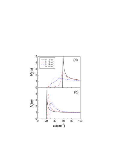
Figure 4: The evolution of the low-temperature densities of states with the interband scattering rate $\Gamma$ in a strong coupling two-band Eliashberg model at $T/T_{\mathrm{c}}=0.1$. The upper panel a) shows the superconducting DOS for the $\sigma$-band, the lower b) the same for the $\pi$-band.

Fig. 5 shows the evolution of the superconducting DOS with temperature for a fixed values of the interband scattering rate $\Gamma$ = 10 cm^-1. One can see that at finite temperature the densities of states in both bands become gapless: In addition to the states at the energy range between the $\pi$-band and the $\sigma$-band gap, states appear down to lowest energies due to thermal phonons. Such gapless behavior is most pronounced close to $T_{\mathrm{c}}$. In the isotropic single-band superconductor, this thermal effect in the strong-coupling regime was demonstrated earlier in Ref. Mikhail, . Note, that the shape and temperature dependence of the superconducting DOS are very different compared to the sum of two BCS-like densities of states. This is particularly pronounced for the $\sigma$-band. Therefore, one would expect a non-BCS temperature behavior in the thermodynamical functions.

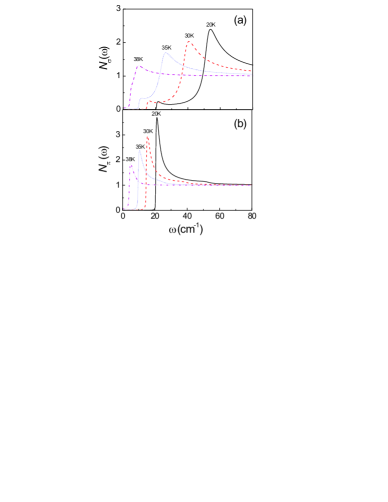
Figure 5: The evolution of the superconducting densities of states with temperature at fixed interband scattering rate $\Gamma$ = 10 cm^-1 in a strong coupling two-band Eliashberg model.

III.2 Thermodynamic Functions

For the numerical calculations for the free energy difference we have used Eq. (II) with parameters described in the previous Section. The entropy difference between the normal and superconducting states is determined by the first derivative of the free energy difference with respect to temperature

$$\Delta S(T)=d\Delta\Omega(T)/dT,$$

and the specific heat difference by the second derivative with respect to temperature

$$\Delta C(T)=Td^{2}\Delta\Omega(T)/dT^{2}.$$

Here we note that taking derivatives from numerically calculated data (as well as from experimental ones) is often a mathematically ill-defined or numerically unstable procedure. Therefore, we used three different schemes to interpolate the numerical data: a) a Chebyshev scheme to interpolate the free energy calculated at non-equidistant points $T_{j}$ = cos($\frac{\pi\,j}{\rm n}$), (j = 0,1, …, n; where n = $T_{c}$/$\Delta T$ is the number of points) and constructing a corresponding matrix n$\times$n operator Chebyshev , b) a polynomial approximation which works well for large temperatures where the densities of states are smooth functions without square-root singularities, and c) an interpolation of the free energy differences by a series of Bessel functions $K_{1}(n\Delta/T)$ similar to the weak-coupling BCS approximation (see e.g., Ref. AGD, ) . The latter captures the superconducting square-root features and works well at low temperatures. The data presented below were chosen such that all three approaches gave similar results.

The specific heat jumps $\Delta C(T_{\mathrm{c}})$ at $T=T_{\mathrm{c}}$ were determined separately by the calculation of the coefficient $\beta=T_{\mathrm{c}}\Delta C(T_{\mathrm{c}})/2$ in the term $\Delta\Omega(T\rightarrow T_{\mathrm{c}})=\beta(1-T/T_{\mathrm{c}})^{2}$.

First, we consider the case without interband impurity scattering (’clean’ case $\Gamma=0$). The expression for $\Delta\Omega(T)$ (see Eq. II) consists of two terms containing $N_{i}(0)$, the renormalization factor $Z_{i}$, and the order parameter $\Phi_{i}$ (or the energy gap $\Delta_{i}=\Phi_{i}/Z_{i}$) for each band separately. These terms reflect the partial contributions of each band to the total free energy (cf. upper panel of Fig. 6). One sees that the $\pi$-band gives a negative contribution to the free energy over the full temperature range. This surprising observation reflects the fact that creation of the superconducting state in the $\pi$-band and, since the superconducting state in the $\pi$-band is induced by the occurrence of superconductivity in the strongly interacting $\sigma$-band, costs energy.

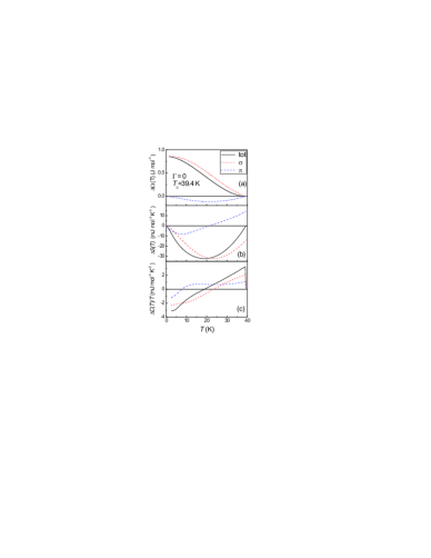
Figure 6: Partial and total contributions to the free energy ($\Delta\Omega$), the entropy ($\Delta S$) and the heat capacity $\Delta C/T$ in the clean case.

The coupling due to the nonzero off-diagonal elements of the electron-phonon interaction is the reason for the same critical temperature $T_{\mathrm{c}}$ and the induced superconducting order parameter in the $\pi$-band. But the analogy to two-independent contributions to the free energy is not fully applicable. The partial $\Delta\Omega_{i}$’s near $T_{\mathrm{c}}$ behave as $O(T_{\mathrm{c}}-T)$ instead of $\Delta\Omega_{tot}\varpropto O((T_{\mathrm{c}}-T)^{2})$, according to the requirements of a mean field theory. In the middle panel of Fig. 6 one can further see that the entropies $\Delta S_{\sigma,\pi}(T_{\mathrm{c}})$ have finite values, whereas only $\Delta S_{tot}(T_{\mathrm{c}})\equiv 0$, as required by the third law of thermodynamics. According to this one has to consider only the total thermodynamic functions as physical ones.

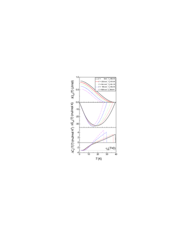
Figure 7: Total contributions to the free energy ($\Delta\,\Omega$), the entropy ($\Delta\,S$) and the heat capacity $\Delta\,C\,/\,T$ for various impurity scattering rates $\Gamma$.

Effects of interband impurity scattering on thermodynamic functions are shown in Fig. 7. The reduced specific heat jumps $\Delta C(T_{\mathrm{c}})/T_{\mathrm{c}}$ at $T=T_{\mathrm{c}}$ grows monotonically with the increase of $\Gamma$ from $3.24$ mJ mol^-1K^-1 in the clean case Golubov to 4.1 mJ mol^-1K^-1 for $\Gamma$ =1000 cm^-1. These values correspond to ratios $\Delta C(T_{\mathrm{c}})/\gamma(T_{\mathrm{c}})T_{\mathrm{c}}\approx 0.98$ (clean case) and 1.3, which are smaller then the corresponding BCS value of 1.43 in a single band model. At low temperatures the ratio $\Delta C(T)/T$ saturates to the value $\lim_{T\rightarrow 0}(C_{SC}(T)/T-C_{N}(T)/T)=-\gamma_{N}(T=0)=-\gamma_{0}(1+\lambda_{av})=-3.24$ mJ mol^-1K^-2 which is determined by the bare (band) electronic specific heat capacity $\gamma_{0}=2\pi^{2}k_{B}^{2}(N_{\sigma}(0)+N_{\pi}(0))/3,$ and the average coupling constant

$$\lambda_{av}=\frac{N_{\sigma}(0)(\lambda_{\sigma\sigma}+\lambda_{\sigma\pi})+N_{\pi}(0)(\lambda_{\pi\sigma}+\lambda_{\pi\pi})}{N_{\sigma}(0)+N_{\pi}(0)},$$

and does not depend on impurities.

IV Eliashberg versus Two-Band $\alpha$-model

Since the two-band $\alpha$-model has been widely used to analyze the experimental heat capacity data of MgB₂ it was interesting to see to which extend a two-gap $\alpha$-model can reproduce the Eliashberg results and, if so, how the corresponding parameters compare with those identified from the Eliashberg calculations.

The $\alpha$-model originally introduced by Padamsee et al., in close analogy to the BCS theory, assumes a BCS temperature dependence of the superconducting gap. The magnitude of superconducting gap at $T$ = 0 is introduced as an adjustable parameter $\alpha$ (from which the $\alpha$–model received its name)Padamsee . The parameter $\alpha$ is defined according to

$$\Delta(T)\,=\,(\alpha\,/\,\alpha_{\mathrm{BCS}})\,\Delta_{\mathrm{BCS}}$$ (9)

with $\alpha_{\mathrm{BCS}}$ = $\Delta_{\mathrm{BCS}}(0)$ / $k_{\mathrm{B}}T_{\mathrm{c}}$ = 1.764 being the weak-coupling value of the gap ratio.

Within the scope of the $\alpha$-model the free energy $F_{\mathrm{S}}$ in the superconducting state can be written as

$$\Omega_{\mathrm{S}}(T)\,=\,2\,N(0)\,\int\limits_{0}^{\infty}\,d\epsilon\,\left\{2\,k_{\mathrm{B}}T\,\ln[1\,-\,f(E)]-\frac{1}{2}\,\frac{(E\,-\,\epsilon)^{2}}{E}\,-\,\frac{\Delta^{2}\,f(E)}{E}\,\right\}$$ (10)

with $E$ = $\sqrt{\epsilon^{2}\,+\,\Delta^{2}}$ and $N(0)$ being the electron and phonon renormalized band-structure electronic density of states at the Fermi energy.

We subtract the normal state contribution to the free energy which corresponds to $\Delta$ = 0 and introduce the dimensionless parameters $t$ = $T\,/T_{\mathrm{c}}$, $\delta(t)\,=\,\Delta(T)\,=\,\Delta_{\mathrm{0}}$ and $x$ = $\epsilon\,/\,k_{\mathrm{B}}T_{\mathrm{c}}$ and arrive at

$$\Delta\,\Omega(t)\,=\,2\,N(0)\,(k_{\mathrm{B}}T_{\mathrm{c}})^{2}\int\limits_{0}^{\infty}\,dx\,\left\{\,2\,t\,\ln[\frac{1\,-\,f(y,\alpha)}{1\,-\,f(x)}]-\frac{1}{2}\,\frac{(y\,-\,x)^{2}}{y}\,-\,\frac{\alpha^{2}\,\delta(t)^{2}\,f(y,\alpha)}{y}\,\right\}$$ (11)

where $y\,=\,\sqrt{x^{2}\,+\,\alpha^{2}\delta(t)^{2}}$, $f(y,\alpha)\,=\,1/[1\,+\,$exp$(y/t)]$, and $f(x)\,=\,f(y,\alpha\,=\,0)\,=\,1/[1+$exp$(x/t)]$

The electronic entropy in the superconducting state is obtained from the first derivative of the free energy with respect to temperature and can be written as

$$S_{\mathrm{el}}(t)\,/\,\gamma\,T_{\mathrm{c}}=-(3/\pi^{2})\,\int\limits_{0}^{\infty}\,dx\left\{f(y,\alpha)\text{ln}\,f(y,\alpha)\,+\,(1\,-\,f(y,\alpha))\text{\thinspace ln\thinspace}(1\,-\,f(y,\alpha))\right\}$$ (12)

wherein the normal-state electronic specific heat capacity (’Sommerfeld - term’) is given by $\gamma$=$\frac{2}{3}\,N(0)\,\pi^{2}\,k_{\mathrm{B}}$.

The electronic heat capacity $C_{\mathrm{el}}$ is calculated from Eq. (12) according to

$$C_{\mathrm{el}}\,/\gamma\,T_{\mathrm{c}}\,=\,t\,(d/dt)\,S_{\mathrm{el}}\,/\,\gamma\,T_{\mathrm{c}}$$ (13)

To compare the Eliashberg results with the two-gap $\alpha$-model approximation we have developed least-squares refinement codes to fit the entropy (Eq. 12) and the heat capacity (Eq. 13) with an $\alpha$-model which linearly superposes the contributions from the $\sigma$ and the $\pi$ electronic system. For the temperature dependence of the reduced gap $\delta(T)$ = $\Delta(T)$ / $\Delta(0)$ we adopted the tabulated values provided by Mühlschlegel Muhlschlegel . For the analytical calculations we used a polynomial fit of the these data.

The heat capacity was calculated from Eq. 13 using an appropriate numerical difference quotient as approximation for the derivative with respect to $t$. Integrations in Eq.(12) were performed numerically with a Gaussian quadrature scheme with a cut-off for $x$ $\geq$ 100. Examples for the fits of the entropy and the heat capacity for $\Gamma$ = 0 and $\Gamma$ = 1000 cm^-1 corresponding to $T_{\mathrm{c}}$ = 39.4 K and $T_{\mathrm{c}}$ = 26.5 K, respectively, are displayed in Fig. 8.

To fit the data we varied $\alpha_{i}$ viz. the energy gaps $\Delta_{i}(T)$ and the Sommerfeld constants $\gamma_{i}$ ($i\,=\,\sigma,\pi$) and a single critical temperature $T_{c}$. All results are compiled in Table 1. Fig. 10 displays the fitted gaps versus $T_{c}$ viz. the interband scattering parameter $\Gamma$.

Attempts to fit also the total energy were less successful and provided results inconsistent with the results of the entropy and heat capacity fits. In these fits we observed a tendency to converge to essentially a single-band model with an averaged gap somewhat above the weak coupling BCS result of $\Delta(0)\,/\,k_{B}T_{c}$ = 1.76. Calculations of the free energies with the $\alpha_{i}$ and $\gamma_{i}$ parameters obtained from the fits to the entropies and heat capacities reproduced the Eliashberg free energies equally well as obtained from the fits of Eq. 10. A closer inspection revealed that characteristic differences for various $\Gamma$ are only visible at small temperatures ($<T_{c}$/5) where the free energy levels to saturation. The fits apparently are not sensitive enough to catch these slight deviations at a satisfying level.

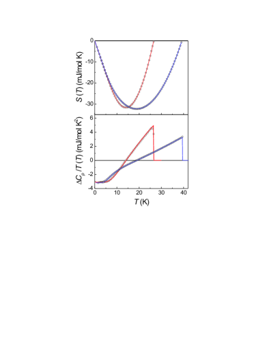
Figure 8: (solid lines) Fits of the Eliashberg entropies and the heat capacities for $\Gamma$ = 0 ($T_{c}$=39.4 K) and $\Gamma$ = 1000 cm^-1 ($T_{c}$=26.5 K) with the $\alpha$-model (Eq. 12 and Eq. 13. For both entropy data sets ($\Gamma$ = 0 cm^-1 ($\circ$) and 1000 cm^-1 ($\square$) and the heat capacity data set with $\Gamma$=0 cm^-1 ($\circ$) a fit with the two-band $\alpha$-model was carried out. The fit of the heat capacity data for $\Gamma$= 1000 cm^-1 ($\square$) was performed with a single-band $\alpha$-model alone.

Table 1 compiles the parameters obtained from the fits of the entropies and the heat capacities. The results are largely independent of whether they are obtained from fits of the entropy or the heat capacity. In general, gaps obtained by fitting of the entropy are closer to the Eliashberg (Matsubara) gaps. Fits in the clean case ($\Gamma$ $\rightarrow$ 0) readily converged with the parameters listed in Table 1. For large values of $\Gamma$, convergence of the fits of the heat capacities with the two-band model were less stable and fits with a single-band model in some cases proved to be more conclusive.

$T_{\mathrm{c}}$ (K)	$\Gamma$ (cm-1)	source	$\Delta^{Eliash}_{\sigma}$ (meV)	$\Delta_{\sigma}$ (meV)	$\Delta^{Eliash}_{\pi}$ (meV)	$\Delta_{\pi}$ (meV)	$\gamma_{\sigma}$/ $\gamma_{\pi}$
		S		7.48		2.88	0.72
39.4	0	C	7.04	7.16	2.67	2.51	0.74
		S		6.97		3.12	0.63
38.1	10	C	6.51	7.00	2.92	3.15	0.62
		S		6.71		3.40	0.64
36.9	23.8	C	6.12	6.39	3.14	3.05	0.67
		S		6.34		3.58	0.53
35.5	40	C	5.77	6.30	3.36	3.58	0.52
		S		5.68		3.63	0.66
34.0	64.4	C	5.47	4.57	3.56	-	-
		S		5.45	1.38		0.60
32.5	100	C	5.95	4.51	3.57	-	-
		S		5.02		3.92	0.80
30.1	196	C	4.80	4.49	3.97	-	-
		S		4.44		3.59	2.7
26.6	1000	C	4.23	4.30	4.09	-	-

Table 1: Critical temperatures $T_{\mathrm{c}}$, $\Delta_{i}$ and Sommerfeld parameters $\gamma_{i}$ as obtained from least-squares fit of the polynom interpolated Eliashberg entropies (S) and the heat capacities (C) by a two-band $\alpha$–model. $\Gamma$ is the interband scattering parameter. The sum $\gamma$ = $\gamma_{\sigma}+\gamma_{\pi}$ of the fitted Sommerfeld terms was found to be constant within 3 %. For comparison the Eliashberg (Matsubara) gaps (solutions of Eq. 3) as displayed in Fig. 10 are listed.

In Fig. 9 we show the total and the partial contributions to the free energy, entropy and the heat capacity calculated according to the $\alpha$-model using the fitted parameters given in Table 1 for $\Gamma$ = 0 ($T_{c}$ = 39.4 K). The $\alpha$-model describes the total heat capacity rather well. There are subtle differences in the partial $\pi$ and $\sigma$ contributions below $T\approx$ 10 K. These difference are also reflected in the fitted ratios of the Sommerfeld constants ($\gamma_{\sigma}$/$\gamma_{\pi}$)_fit which deviates markedly from the ratio of the phonon renormalized Sommerfeld terms used for the Eliashberg calculations, ($\gamma_{\sigma}$/$\gamma_{\pi}$) = $N_{\sigma}(0)/N_{\pi}(0)((1+\lambda_{\sigma\sigma}+\lambda_{\sigma\pi})/(1+\lambda_{\pi\pi}+\lambda_{\pi\sigma}))\approx 1$.

Naturally, since within the scope of the $\alpha$-model all partial contributions are positive definite, the negative $\pi$ partial free energy and the sign change of the $\pi$ partial entropy (compare to Fig.6) cannot be reproduced.

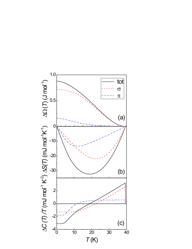
Figure 9: Partial and total contributions to the free energy ($\Delta\Omega$), the entropy ($\Delta S$) and the heat capacity $\Delta C/T$ in the clean case calculated with the two-band $\alpha$-model.

Finally, Fig. 10 shows the superconducting gaps as obtained from the fits in comparison with the Eliashberg calculations. The agreement is fairly good for higher $T_{c}$. Deviations are seen for $T\cong$ 33 K for the gaps gained from the fits of the heat capacities, while the gaps received from the fits of the entropy rather well follow the Matsubara calculations and the merging point of both gaps at the weak coupling value is also well reproduced.

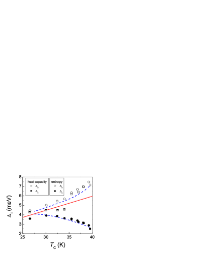
Figure 10: Superconducting gaps $\Delta(0)_{\sigma}$ and $\Delta(0)_{\pi}$ as obtained from the fits of the Eliashberg entropies ($\circ$) and the heat capacities ($\Box$) with the two-band $\alpha$-model (Eq. 12 and 13). Gap data gained from fits of the heat capacities for $T_{c}<35K$ were obtained from a fit with a single one-band $\alpha$-model. The (red) solid line shows the weak coupling result $\Delta_{\mathrm{BCS}}$ = 1.76 $T_{c}$. The dashed (blue) lines represents the results of the Matsubara calculations of $\Delta_{\sigma}(\omega_{n}=\pi T)$ and $\Delta_{\pi}(\omega_{n}=\pi T)$.

V Conclusion

In summary, using the Eliashberg approach, we have studied the behavior of the superconducting density of states, energy gaps, free energy, entropy and specific heat in a strongly-coupled two-band superconductor with interband impurity scattering. We have demonstrated strong modifications of the densities of states by interband scattering and have shown how thermal effects modify these results. We have calculated the temperature dependencies of the free energy, the entropy and the specific heat and the specific jump at $T_{c}$ as a function of interband scattering rates and performed a detailed comparison of the phenomenological two-band $\alpha$-model with the Eliashberg results. We have shown that despite strong modifications of the DOS by interband scattering, the $\alpha$-model approach is sufficiently accurate and can - as a first approximation - be used to extract gap values from experimental heat capacity or entropy data.

Interband scattering alone, however, is not sufficient to model the decrease of $T_{c}$ observed for Al and C doped samples Mg_1-xAl_x(B_1-yC_y)₂. As demonstrated recently, the decrease of $T_{c}$ can rather be understood in terms of a band filling effect due to the electron doping by Al and C and a concomitant scaling of the electron-phonon coupling constant $\lambda$ by the variation of the density of states as a function of electron doping PRL2005 . Compensation of band filling and interband scattering effects shifts the merging point of the $\sigma$ and $\pi$ gaps to higher doping concentrations and lower $T_{c}$’s than expected based on interband scattering considerations alone. Only the combination of interband scattering with band filling effects allowed us to model the nearly constant $\pi$ gap and the decreased critical temperature and increased doping concentrations at which the $\sigma$ and $\pi$ gaps finally merge.

Appendix

In order to calculate the thermodynamic potential $\Omega$ for a superconductor with strong electron-phonon coupling and nonmagnetic impurities, we use a general expression for the electron Matsubara $2\times 2$ matrix Green function

$$\overset{\wedge}{G_{j}}(p)=-\frac{iZ_{jn}^{S}\omega_{n}\hat{\tau}_{0}+\xi_{j}(\mathbf{p})\hat{\tau}_{3}+\Phi(p)\hat{\tau}_{2}}{(Z_{jn}^{S}\omega_{n})^{2}+\xi_{j}^{2}(\mathbf{p})+\Phi^{2}(p)},$$ (14)

where $\xi_{j}(\mathbf{p})$ is the bare spectrum ($p=\{j,\mathbf{p},\omega_{n}\},$ with band index $j$ and momentum $\mathbf{p}$). Pauli matrices $\hat{\tau}$ correspond to Nambu space. This Green function obeys the Eliashberg equations, which allows us to express the potential $\Omega$ directly through it as will be shown below.

The thermodynamic potential $\Omega$ can always be expressed by the electron Green function by means of integration over the electron charge. Using e.g. Eq.(16.9) from Ref. AGD, one obtains

$$\begin{array}[]{c}\Omega=\Omega_{e}^{(0)}+\Omega_{ph}^{(0)}+T\sum_{p}\int\limits_{0}^{1}\frac{dx}{x}\,\text{tr}\left[\overset{\wedge}{G}_{(0)}^{-1}(p)\left(\overset{\wedge}{G}(x,p)-\overset{\wedge}{G}_{(0)}(p)\right)\right]=\\ \Omega_{\text{ }e}^{(0)}+\Omega_{ph}^{(0)}+T\sum_{p}\int\limits_{0}^{1}\frac{dx}{x}\,\text{tr}\left[\overset{\wedge}{\Sigma}(x,p)\overset{\wedge}{G}(x,p)\right]\end{array}$$ (15)

where $x$ is a dimensionless factor. $\overset{\wedge}{G}(x,p)$ and $\overset{\wedge}{\Sigma}(x,p)$ are the exact electron Green function and the self-energy for the case when the electron charge has the value $xe$. $\overset{\wedge}{G_{(0)}}$($p$) is the Green function for zero coupling constant.

The electron-phonon contribution can be expressed in terms of electron and phonon Green functions by means of Eliashberg equation:

$$\overset{\wedge}{\Sigma}(x,t_{M},\mathbf{r})=T\sum_{\omega_{n},\mathbf{p},j=\pi,\sigma}\overset{\wedge}{\Sigma}(\omega_{n},\mathbf{p},j)e^{i\mathbf{p\cdot r}-i\omega_{n}t_{M}}=x^{2}\hat{\tau}_{3}\overset{\wedge}{G}(x,t_{M},\mathbf{r})\hat{\tau}_{3}D(t_{M},\mathbf{r}),$$ (16)

where $D(t_{M},\mathbf{r})=g^{2}D_{(0)}(t_{M},\mathbf{r})+D_{imp}(t_{M},\mathbf{r})$. $D_{(0)}(t_{M},\mathbf{r})$ is the phonon Green function expressed in coordinate representation,$-1/T\leq t_{M}\leq 1/T$ is the Matsubara time. Here we suppose that the phonon Green function is independent of the coupling constant in the adiabatic approximation. This is the usual approximation, which is related to the fact that the electron-phonon Hamiltonian contains the phonon spectrum already renormalized due to the electron-phonon interaction and one should not take this renormalization into account once more. The second term corresponding to impurity scattering is considered in the Born approximation, where $D_{imp}(t_{M},\mathbf{r})\varpropto e^{2}$. Below we follow Ref. gd, . Making use of Eq. (16) we can derive the simple identity:

$$\text{tr}\left(\overset{\wedge}{\Sigma}(x)\overset{\wedge}{G}(x)-\frac{x}{2}\frac{d\overset{\wedge}{\Sigma}(x)}{dx}\overset{\wedge}{G}(x)\right)=-\text{tr}\left(\frac{x}{2}\frac{d\overset{\wedge}{G}(x)}{dx}\overset{\wedge}{\Sigma}(x)\right),$$

which allows us to rewrite Eq. (15) in the coordinate representation ($r=\{t_{M},\mathbf{r}\}$)

$$\Omega=\Omega_{\text{ }e}^{(0)}+\Omega_{ph}^{(0)}+\int dr\int\limits_{0}^{1}\frac{dx}{x}\text{tr}\left(\overset{\wedge}{\Sigma}(x)\overset{\wedge}{G}(x)-\frac{x}{2}\frac{d\overset{\wedge}{\Sigma}(x)}{dx}\overset{\wedge}{G}(x)+\frac{x}{2}\frac{d\overset{\wedge}{\Sigma}(x)}{dx}\overset{\wedge}{G}(x)\right)=$$

$$=\Omega_{\text{ }e}^{(0)}+\Omega_{ph}^{(0)}-\int dr\int\limits_{0}^{1}\frac{dx}{x}\,\text{tr}\left(\frac{x}{2}\frac{d\overset{\wedge}{G}(x)}{dx}\overset{\wedge}{\Sigma}(x)\right)+\int dr\int\limits_{0}^{1}\frac{dx}{x}\text{tr}\left(\frac{x}{2}\frac{d\overset{\wedge}{\Sigma}(x)}{dx}\overset{\wedge}{G}(x)\right)=$$

$$=\Omega_{\text{ }e}^{(0)}+\Omega_{ph}^{(0)}-\frac{1}{2}\int dr\int\limits_{0}^{1}dx\,\text{tr}\left(\frac{d\overset{\wedge}{G}^{-1}(x)}{dx}\overset{\wedge}{G}(x)\right)-\frac{1}{2}\int dr\int\limits_{0}^{1}dx\,\text{tr}\left(\frac{d\overset{\wedge}{G}(x)}{dx}\left(\overset{\wedge}{G}_{(0)}^{-1}-\overset{\wedge}{G}^{-1}(x)\right)\right)$$

we can now perform the integration over $x$ exactly and find after Fourier transformation the required expression:

$$\Omega=\Omega_{e}^{(0)}+\Omega_{ph}^{(0)}+T\sum_{p}\left(\ln\det\overset{\wedge}{G}\right)-\int dr\left(\ln\det\overset{\wedge}{G}_{(0)}\right)-\frac{T}{2}\sum_{p}\text{tr}\left(\overset{\wedge}{G}_{(0)}^{-1}\overset{\wedge}{G}-\overset{\wedge}{1}\right).$$ (17)

This expression is valid provided that the Green functions $\overset{\wedge}{G}$ satisfy the Eliashberg equations.

For the difference of free energies in the S and N-states we have after the Fourier transformation

$$\Delta\Omega=T\sum_{j,\mathbf{p},\omega_{n}}\left(\ln\frac{\det\overset{\wedge}{G}_{j}}{\det\hat{G}^{N}_{j}}\right)-\frac{T}{2}\sum_{j,\mathbf{p},\omega_{n}}\text{tr}\left(\overset{\wedge}{G_{0}}_{(j)}^{-1}\left(\overset{\wedge}{G_{j}}-\overset{\wedge}{G^{N}_{j}}\right)\right),$$ (18)

where $\overset{\wedge}{G^{N}}$ is given by

$$\overset{\wedge}{G^{N}_{j}}=-\frac{iZ_{jn}^{N}\omega_{n}\hat{\tau}_{0}+\xi_{j}(\mathbf{p})\hat{\tau}_{3}}{(Z_{jn}^{N}\omega_{n})^{2}+\xi_{j}^{2}(\mathbf{p})}$$

Eq.18 is the sum of Green functions in different bands. Finally $\Delta\Omega$ can be expressed as

$$\Delta\Omega=-T\sum_{\omega_{n}}\sum_{j,\mathbf{p}}\ln\left[\frac{(Z_{jn}^{S}\omega_{n})^{2}+\xi_{j}^{2}(\mathbf{p})+\Phi_{jn}^{2}}{(Z_{jn}^{S}\omega_{n})^{2}+\xi_{j}^{2}(\mathbf{p})}\right]+$$

$$+T\sum_{\omega_{n}}\sum_{j,\mathbf{p}}\left[\frac{-Z_{jn}^{S}\omega_{n}^{2}+(Z_{jn}^{S}\omega_{n})^{2}+\Phi_{jn}^{2}}{(Z_{jn}^{S}\omega_{n})^{2}+\xi_{j}^{2}(\mathbf{p})+\Phi_{jn}^{2}}-\frac{-Z_{jn}^{N}\omega_{n}^{2}+(Z_{jn}^{N}\omega_{n})^{2}}{(Z_{jn}^{N}\omega_{n})^{2}+\xi_{j}^{2}(\mathbf{p})}\right].$$

After integration with respect to the momentum we obtain the expression

$$\Delta\Omega = -2\pi T\sum_{j,\omega_{n}}^{\left|\omega_{c}\right|}N_{j}(0)\left[\sqrt{(Z_{jn}^{S}\omega_{n})^{2}+\Phi_{jn}^{2}}-\left|Z_{jn}^{N}\omega_{n}\right|\right]+$$

$$+\pi T\sum_{j,\omega_{n}}^{\left|\omega_{c}\right|}N_{j}(0)\left[\frac{-Z_{jn}^{S}\omega_{n}^{2}+(Z_{jn}^{S}\omega_{n})^{2}+\Phi_{jn}^{2}}{\sqrt{(Z_{jn}^{S}\omega_{n})^{2}+\Phi_{jn}^{2}}}-\frac{-Z_{jn}^{N}\omega_{n}^{2}+(Z_{jn}^{N}\omega_{n})^{2}}{\left|Z_{jn}^{N}\omega_{n}\right|}\right]$$

This expression does not contain any impurities directly. The effect of intraband impurities cancels from Eqs. (3-7). Also $Z^{S}$, $Z^{N}$, and $\Phi$ do not depend on intraband scattering, however these functions are dependent on interband impurity scattering.

The final answer is the expression given in Eq. (1)

$$\Delta\Omega=-\pi T\sum_{j=\sigma,\pi}\sum\limits_{n=-\omega_{c}}^{\omega_{c}}N_{j}(0)\left\{|Z_{jn}^{N}\omega_{n}|-\left|\omega_{n}\right|-\frac{2(Z_{jn}^{S}\omega_{n})^{2}-2\omega_{n}^{2}+2\Phi_{jn}^{2}}{|\omega_{n}|+\sqrt{(Z_{jn}^{S}\omega_{n})^{2}+\Phi_{jn}^{2}}}+\right.$$

$$\left.+\frac{(Z_{jn}^{S}\omega_{n})^{2}-Z_{jn}^{S}\omega_{n}^{2}+\Phi_{jn}^{2}}{\sqrt{(Z_{jn}^{S}\omega_{n})^{2}+\Phi_{jn}^{2}}}\right\}.$$

References

- (1) J. Nagamatsu, N. Nakagawa, T. Muranaka, Y. Zenitani, and J. Akimitsu, Nature (London) 463, 401 (2001).
- (2) H. Suhl, B. T. Matthias, and L. R. Walker, Phys. Rev. Lett. 3, 552 (1959).
- (3) V.A. Moscalenko, Fiz. Met. Metalloved.8, 503 (1959).
- (4) P. B. Allen and B. Mitrovi, Solid State Physics, edited by F. Seitz, D. Turnbull, and H. Ehrenreich, (Academic, New York, 1982, Vol. 37, p. 1.)
- (5) L. Y. L. Shen, N. M. Senozan, and N. E. Phillips, Phys. Rev. Lett. 14, 1025 (1965)
- (6) R. Radebaugh and P. H. Keesom, Phys. Rev. 149, 209 (1966).
- (7) G. Binnig, A. Baratoff, H. E. Hoenig, and J. G. Bednorz, Phys. Rev. Lett. 45, 1352 (1980).
- (8) See special issue on MgB2, edited by G. Crabtree, W. Kwok, P. C. Canfield, and S. L. Bud’ko [Physica (Amsterdam) C 385, 1 (2003)].
- (9) J. Kortus, I. I. Mazin, K. D. Belashchenko, V. P. Antropov, and L. L. Boyer, Phys. Rev. Lett. 86, 4656 (2001).
- (10) J. M. An and W. E. Pickett, Phys. Rev. Lett. 86, 4366 (2001).
- (11) A.Y. Liu, I.I. Mazin, J. Kortus, Phys. Rev. Lett. 87, 87005 (2001).
- (12) Y. Kong, O. V. Dolgov, O. Jepsen, and O. K. Andersen, Phys. Rev. B64, 020501(R) (2001).
- (13) K. B. Bohnen, R. Heid, and B. Renker, Phys. Rev. Lett. 86, 5771 (2001).
- (14) H. J. Choi, M. L. Cohen, S. G. Louie, Nature (London) 418, 758 (2002); Physica C385, 66 (2003).
- (15) K. Kunc, I. Loa, K. Syassen, R. K. Kremer, and K. Ahn, J. Phys: Condens. Matter 13, 9945 (2001).
- (16) A. A. Golubov, J. Kortus, O. V. Dolgov, O. Jepsen, Y. Kong, O. K. Andersen, B. J. Gibson, K. Ahn, and R. K. Kremer, J. Phys: Condens. Matter 14, 1353 (2002).
- (17) A. A. Golubov and I. I. Mazin, Phys. Rev. B 55, 15146 (1997).
- (18) N. Schopohl and K. Scharnberg, Solid State Commun. 22, 371 (1977).
- (19) A. Brinkman, A. A. Golubov, H. Rogalla, O. V. Dolgov, J. Kortus, Y. Kong, O. Jepsen, and O. K. Andersen. Phys. Rev. B 65, 180517 (2002).
- (20) I. I. Mazin, O. K. Andersen, O. Jepsen, O. V. Dolgov, J. Kortus, A. A. Golubov, A. B. Kuz’menko, and D. van der Marel, Phys. Rev. Lett. 89, 107002 (2002).
- (21) S. Agrestini, D. Di Castro, M. Sansoni, N. L. Saini, A. Saccone, S. De Negri, M. Giovannini, M. Colapietro, and A. Bianconi, J. Phys.: Condens. Matter 13, 11689 (2001).
- (22) F. Bouquet, R. A. Fisher, N. E. Phillips, D. G. Hinks, and J. Jorgensen, Phys. Rev. Lett. 87, 047001 (2001).
- (23) Y. Wang, T. Plackowski, and A. Junod, 2001 Physica C355, 179 (2001).
- (24) J. Y. Xiang, D. N. Zheng, J. Q. Li, L. Li, L. Lang, H. Chen, C. Dong, G. C. Che, Z. A. Ren, H. H. Qi, Y. Tian, Y. M. Ni, and Z. X. Zhao, Phys. Rev. B 65, 214536 (2002).
- (25) J. Q. Li, L. Li, F. M. Liu, C. Dong, J. Y. Ziang, and Z. X. Zhao, Phys. Rev. B 65, 132505 (2002).
- (26) S. Margadonna, K. Prassides, I. Arvanitidis, M. Pissas, G. Papavassiliou, and A. N. Fitch, Phys. Rev. B66, 014518 (2002).
- (27) G. Papavassiliou, M. Pissas, M. Karayanni, M. Fardis, S. Koutandos and K. Prassides, Phys. Rev. B66, 140515 (2002).
- (28) A. Bianconi, S. Agrestini, D. Di Castro, G. Campi, Z. Zangari, N. L. Saini, A. Saccone, S. De Negri, M. Giovannini, G. Profeta, A. Continenza, G. Satta, S. Massidda, A. Cassetta, A. Pifferi, and M. Colapietro, Phys. Rev. B65, 174515 (2002).
- (29) O. de la Pena, A. Aguayo, and R. de Coss, Phys. Rev. B66, 012511 (2002).
- (30) P. Postorino, A. Congeduti, P. Dore, A. Nucara, A. Bianconi, D. Di Castro, S. De Negri, and A. Saccone, Phys. Rev. B 65, 020507 (2001).
- (31) D. Di Castro, S. Agrestini, G. Campi, A. Cassetta, M. Colapietro, A. Congeduti, A. Continenza, S. De Negri, M. Giovannini, S. Massidda, M. Tardone, A. Pifferi, P. Postorino, G. Profeta, and A. Saccone, Europhys. Lett. 58, 278 (2002).
- (32) M. Putti, M. Affronte, P. Manfrinetti, and A. Palenzona, Phys. Rev. B 68, 094514 (2003).
- (33) R. A. Ribeiro, S. L. Bud’ko, C. Petrovic, and P. C. Canfield, Physica C384, 227 (2003); R. A. Ribeiro, S. L. Budko, C. Petrovic, and P. C. Canfield, Physica C385, 16 (2003).
- (34) H. Schmidt, K. E. Gray, D. G. Hinks, J. F. Zasadzinski, M. Avdeev, J. D. Jorgensen, and J. C. Burlea, Phys. Rev. B68, 060508(R) (2003).
- (35) K. Papagelis, J. Arvanitidis, K. Prassides, A. Schenck, T. Takenbou, and Y. Iwasa, Europhys. Lett. 61, 254 (2003).
- (36) Z. Hoanov, P. Szab, P. Samuely, R. H. T. Wilke, S. L. Bud’ko, and P. C. Canfield, Phys. Rev. B 70, 064520 (2004).
- (37) R. S. Gonnelli, D. Daghero, A. Calzolari, G.A. Ummarino, V. Dellarocca, V. A. Stepanov, S. M. Kazakov, N. Zhigadlo, J. Karpinski, Phys. Rev. B 71, 060503(R) (2005).
- (38) Yuxing Wang, F. Bouquet, I. Sheikin, P. Toulemonde, B. Revaz, M. Eisterer, H. W. Weber, J. Hinderer, and A. Junod, J. Phys.: Condens. Matter 15, 883 (2003).
- (39) J. Kortus, O. V. Dolgov, R. K. Kremer, and A. A. Golubov, Phys. Rev. Lett. 94, 027002 (2005).
- (40) G.A. Ummarino, R.S. Gonnelli, S. Massidda, and A. Bianconi, Physica C407, 121 (2004).
- (41) A. Bussmann-Holder and A. Bianconi, Phys. Rev B67, 132509 (2003).
- (42) V. L. Pokrovsky, Zh. Eksp. Teor. Fiz. 40, 641 (1961) [Sov.Phys. JETP 13, 447 (1961)]; V. L. Pokrovsky and M. S. Ryvkin, Zh. Eks. Teor. Fiz. 43, (1962) [Sov. Phys. JETP 16, 67 (1963)].
- (43) V. A. Moscalenko, M. E. Palistrant, and V. M. Vakalyuk, Sov. Phys. Uspekhi 161, 155 (1991)
- (44) M. E. Palistrant, F. G. Kochorbe, Physica C 194, 351-362, (1992).
- (45) T. Soda and Y. Wada, Prog. Theor. Phys. 36, 1111 (1966).
- (46) B. T. Geilikman, R. O. Zaitsev and V. Z. Kresin, Fiz. Tverd. Tela (Leningrad) 9, 821 (1967); [Sov. Phys. Solid State 9, 642 (1967)].
- (47) L. Shen, N. Sonzoan, and N. E. Phillips, Phys. Rev. Lett. 14, 1025 (1965).
- (48) V. Z. Kresin, J. Low Temp. Phys. 11, 519 (1973).
- (49) H. Chi and J. P. Carbotte, Physica C169, 55 (1990).
- (50) T. M. Mishonov and E. Penev, Int. J. Mod. Phys. B 16, 3573 (2002), T. M. Mishonov, S.-L. Drechsler, and E. Penev, Mod. Phys. Lett. 17, 755 (2003), T. M. Mishonov, V. L. Pokrovsky, and H. Wei, Int. J. Mod. Phys. B17, 755 (2003); T. M. Mishonov, E. S. Penev, J. O. Indekeu, V. L. Pokrovsky, Phys. Rev. B68, 104517 (2003); T. M. Mishonov, S. I. Klenov, and E. S. Penev, Phys. Rev. B70, 024520 (2005).
- (51) V. P. Ramunni, G. M. Japiassu, A. Troper, Physica C364-365, 190 (2001); Physica C408-410, 358 (2004).
- (52) N. Nakai, M. Ichioka, and K. Machida, Int. J. Mod. Phys. B16, 3573-3586, (2002).
- (53) N. Kristoffel, T. Ord, and K. Rago, Europhys. Lett. 61, 109 (2003); T. Ord, N. Kristoffel, Physica C370, 17 (2002)
- (54) K. Watanabe and T. Kita, J. Phys. Soc. Japan 73, 2239 (2004)
- (55) M. E. Palistrant, preprint cond-mat /0312302 (unpublished).
- (56) J. P. Carbotte, Rev. Mod. Phys. 62, 1027 (1990).
- (57) M. Zehetmayer, H. W. Weber, and E. Schachinger J. Low Temp. Phys. 133, 407 (2003)
- (58) B. Mitrovic J. Phys.: Condens. Matter 16, 9013 (2004).
- (59) E. J. Nicol and J. P. Carbotte, Phys. Rev. B71, 054501 (2005).
- (60) S. V. Shulga in: ’Material Science, Fundamental Properties and Future Electronic Applications of High-Tc Superconductors’, Kluwer Academic Publishers, Dortrecht, pp. 323-360 (2001).
- (61) A. A. Mikhailovskii, S. V. Shulga, A. E. Karakozov, O. V. Dolgov, and E. G. Maksimov, Solid State Commun. 80, 511 (1991).
- (62) L. N. Trefethen, Spectral methods in matlab, (SIAM, 2000).
- (63) A. A. Abrikosov, L. P. Gor’kov, and I. E. Dzyaloshinskii, Methods of quantum field theory in statistical physics, (Dover, New York, 1969).
- (64) H. Padamsee, J. E. Neighbor, and C. A. Shifman, J. Low Temp. Phys. 12, 387 (1973).
- (65) B. Mühlschlegel, Z. Phys. 155, 313 (1959).
- (66) D.A. Golubev and O.V. Dolgov, 1993 (unpublished)
- (67) R. K. Kremer, B. J. Gibson, and K. Ahn, cond-mat-010243 (unpublished).
- (68) Heat capacity data by Wang et al. Wangirra privately communicated to us. The data were fitted with the Stuttgart version of the phenomenological two-band –model (Ref. condmat, ) allowing for an additional Gaussian broadening of .