Anomalous Tunneling of Bound Pairs in Crystal Lattices

Abstract

A novel method of solving scattering problems for bound pairs on a lattice is developed. Two different break ups of the hamiltonian are employed to calculate the full Green operator and the wave function of the scattered pair. The calculation converges exponentially in the number of basis states used to represent the non-translation invariant part of the Green operator. The method is general and applicable to a variety of scattering and tunneling problems. As the first application, the problem of pair tunneling through a weak link on a one-dimensional lattice is solved. It is found that at momenta close to $\pm\pi$ the pair tunnels much easier than one particle, with the transmission coefficient approaching unity. This anomalously high transmission is a consequence of the existence of a two-body resonant state localized at the weak link.

Introduction. Scattering of bound particle complexes has been a major subject of atomic, molecular and nuclear physics for decades. In “lattice” solid state physics the prime system of interest has been the exciton Davydov1962 ; Knox1963 , in which the constituent particles, an electron and a hole, have different masses. The bound pair of two magnons in lattice magnetism is an example of a complex with equal masses Mattis1981 . In recent years, the concepts of lattice bipolarons BrazKirova1981 ; Heeger1988 ; MicRanRob1990 ; AleMott1994 ; AleKor2002a and bisolitons Davydov1989 have been developed, in particular in relation with high-temperature superconductors and conducting polymers.

Many properties of these particles derive just from their composite nature rather than from the particulars of the binding interaction. They can therefore be studied within the framework of the “generic” two-body system, in which a model potential is introduced to ensure binding, yet the simplicity of the potential enables rigorous analysis of the quantum mechanical problem. This approach has been popular and the physics of two-particle bound complexes in translation invariant lattices is now well-understood, see for example Refs. [Mat1986, ; Viega2002, ; Kor2004, ] and the bibliography therein. Much less is known about non-translation invariant cases. When defects or boundaries are present the two-body problem can no longer be reduced to a one-body problem, which significantly complicates analysis. In continuum physics, scattering of bound pairs was approached from the general three-body formalism Schwebel1956 ; Jasperse1967 ; AleBraKor2002 , although no exact results were obtained beyond the one dimension with delta-function potentials. On a lattice, the previous research was limited to the surface excitonic effects Hizhnyakov1975 ; Gumbs1981 . Bulatov Bulatov1984 ; Bulatov1987 developed a general theory and an efficient numerical procedure to obtain the energy spectra and wave functions of lattice excitons in the presence of a surface.

In this Letter, we extend the method of Refs. [Bulatov1984, ; Bulatov1987, ] to the general scattering problem of lattice bound pairs. The method consists of calculating the full two-particle Green operator $G$ and then acting with it on the wave function of an incident pair $\Psi_{V}$. The core feature of the method is the usage of two different decompositions of the hamiltonian on a zero part and a perturbation. The first decomposition is applied to find $G$ while the second decomposition is used to calculate the scattering amplitudes. The accuracy of the method increases exponentially with the number of lattice sites used to approximate the non-translation invariant part of $G$. As the first application of the method we solve the problem of tunneling of a one-dimensional bound pair through a weak link on a chain. We find that the pair transmission at large lattice momenta is significantly enhanced in comparison with the transmission of a single particle. In fact, the transmission coefficient approaches unity at the Brillouin zone boundary.

Method. The generic model consists of free motion of two particles $H_{0}$, interparticle interaction $V$ (which is usually attractive), and single-particle scattering $U$:

$$H = H_{0}+V+U$$ (1)

$$= H_{V}+U$$ (2)

$$= H_{U}+V.$$ (3)

Here two partial hamiltonians $H_{V}=H_{0}+V$ and $H_{U}=H_{0}+U$ are introduced. Equations (2) and (3) define the two decompositions mentioned above. Using the decomposition (2), the full wave function $\Psi$ satisfies the Schrödinger equation

$$\Psi=\Psi_{V}+G_{V}U\Psi,$$ (4)

where $H_{V}\Psi_{V}=E\Psi_{V}$, $\Psi_{V}$ has the appropriate boundary conditions at infinity, and $G_{V}(E)=(E-H_{V}+i\gamma)^{-1}$ is the Green operator of $H_{V}$. Three other Green operators $G$, $G_{0}$, and $G_{U}$ are defined analogously. In the basis of localized lattice states the Green operators can be represented as ordinary matrices, albeit of infinite size.

Ordinarily, equations like (4) are used to develop perturbative expansions for $\Psi$ from the knowledge of the partial Green operator $G_{V}$. Now suppose that the full Green operator $G$ is known. Since $G=(1-G_{V}U)^{-1}G_{V}$ and $\Psi=(1-G_{V}U)^{-1}\Psi_{V}$, the last term in (4) is re-arranged as follows

$$G_{V}U\Psi = G_{V}U(1-G_{V}U)^{-1}\Psi_{V}$$ (5)

$$= (1-G_{V}U)^{-1}G_{V}U\Psi_{V}=GU\Psi_{V},$$

so that, from Eq. (4)

$$\Psi=\Psi_{V}+GU\Psi_{V}=(1+GU)\Psi_{V}.$$ (6)

Thus if $G$ is known, the full wave function can be found from the last equation by matrix multiplication.

Now comes an important observation. Since $G$ is the full Green operator it does not matter how it is obtained. In particular, one is not obligated to use the same decomposition (2) that has led to Eq. (6). For scattering of bound pairs it is more convenient to use the decomposition (3), which yields

$$G=(1-G_{U}V)^{-1}G_{U}\equiv A^{-1}G_{U}.$$ (7)

The advantage of this approach is that $G_{U}$ is the Green operator of two non-interacting particles, both scattered off the potential $U$. Therefore $G_{U}$ can be calculated as a convolution of two one-particle Green operators $g_{U}$:

$$G_{U}({\bf r}_{1}{\bf r}^{\prime}_{1};{\bf r}_{2}{\bf r}^{\prime}_{2};E)=i\!\!\int^{\infty}_{-\infty}\!\frac{d\epsilon}{2\pi}\,g_{U}({\bf r}_{1}{\bf r}^{\prime}_{1};\epsilon)g_{U}({\bf r}_{2}{\bf r}^{\prime}_{2};E-\epsilon).$$ (8)

In turn, $g_{U}$ follows from solving of a one-particle scattering problem:

$$g_{U}=(1-g_{0}U)^{-1}g_{0},$$ (9)

where $g_{0}=(E-H_{0}+i\gamma)^{-1}$ is the one-particle Green operator of the translation-invariant system. The zero operator $g_{0}$ is most easily calculated from the spectral expansion

$$g_{0}({\bf r},{\bf r}^{\prime};E)=\sum_{\bf k}\frac{e^{i{\bf k}({\bf r}-{\bf r}^{\prime})}}{E-\varepsilon_{\bf k}+i\gamma},$$ (10)

where $\varepsilon_{\bf k}$ is the one-particle spectrum. $G_{U}$ can also be calculated from the two-particle spectral expansion note . Thus the strategy of the present method is to use the decomposition (3) and formulas (7)-(10) to obtain the Green operator $G$, and then use the decomposition (2) and formula (6) to calculate the full wave function $\Psi$ and the scattering coefficients of interest.

Calculation of $(1-G_{U}V)^{-1}$. Once $G_{U}$ is known, the main task is to invert the matrix $A\equiv 1-G_{U}V$, see Eq. (7). The way of calculating $A^{-1}$ is the second key component of the present method. Observe that inverting $(1-G_{U}V)$ is analogous to inverting $(E-H)$, i.e., to calculating a Green operator. Imagine a $G_{U}$ that consists of a translation-invariant part $G^{0}_{U}$ and a perturbation $\delta G=G_{U}-G^{0}_{U}$ which is localized in real space. Then the translation invariant part $(1-G^{0}_{U}V)$ plays the role of the translation invariant part of $(E-H)$ while $\delta GV$ the role of the localized perturbation. Performing the standard transformation one obtains

$$A^{-1}=(1-G^{0}_{U}V-\delta G\>V)^{-1}=(1-B^{-1}\delta G\>V)^{-1}\,B^{-1},$$ (11)

$$B\equiv 1-G^{0}_{U}V.$$ (12)

Thus inversion of $A$ is replaced with two inversions. The first inversion is that of $B$. Since $B$ involves only translation-invariant matrices this is achieved by changing to the quasi-momentum representation in which $B$ is block-diagonal with the block size equal to the range of $V$ Bulatov1987 in relative coordinates. The second inversion is that of $(1-B^{-1}\delta G\>V)$. The latter is the sum of the unit matrix and a matrix localized around the scattering region, which is due to the localization of $\delta G$. Thus only inversion of a finite-size matrix that contains the non-zero elements of $B^{-1}\delta G\>V$ is required. As a result, the abstract task of inverting the infinite matrix $A$ is replaced with two easy-to-perform operations on finite size matrices.

To summarize, the algorithm begins with the calculation of the Green matrix $G_{U}$ from Eqs. (8)-(10). Then $G_{U}$ is separated into the translation-invariant part $G^{0}_{U}$ and the remainder $\delta G$. On the next step, $A^{-1}$ is calculated according to Eq. (11), and then the full Green operator is obtained from Eq. (7). Finally, an unperturbed pair wave function $\Psi_{V}$ is chosen and the scattered wave function is calculated from Eq. (6). This formulation is completely general, and can be applied to a variety of particular cases. One such problem is analyzed below.

A chain with a weak link. Consider a one-dimensional chain characterized by the nearest-neighbor hopping matrix element $t>0$ and the Hubbard-like attraction of strength $|v|>0$. The hopping amplitude between sites $n=0$ and $n=1$ contains an additional element $t^{\prime}$. The resulting hamiltonian reads

$$H = -t\sum_{\langle nn^{\prime}\rangle\sigma}c^{\dagger}_{n\sigma}c_{n^{\prime}\sigma}-|v|\sum_{n}c^{\dagger}_{n\uparrow}c_{n\uparrow}c^{\dagger}_{n\downarrow}c_{n\downarrow}$$ (13)

$$+t^{\prime}\sum_{\sigma}\left(c^{\dagger}_{0\sigma}c_{1\sigma}+c^{\dagger}_{1\sigma}c_{0\sigma}\right),$$

where $\langle nn^{\prime}\rangle$ denotes pairs of nearest neighbor sites. The value $t^{\prime}=0$ corresponds to the absence of any scattering while $t^{\prime}=t$ corresponds to two decoupled semi-infinite chains. A standard solution of the one-particle scattering problems yields the transmission coefficient:

$$\tau_{k}=\frac{(t^{\prime}/t-1)(e^{ik}-e^{-ik})}{e^{-ik}-(t^{\prime}/t-1)^{2}\,e^{ik}},$$ (14)

where $k$ is the one-particle momentum. The modulus of the transmission coefficient $|\tau_{k}|$ is shown in Fig. 1 in bold lines. Note that $\tau_{k}=0$ at $k=0$ or $k=\pi$.

In the absence of scattering ($t^{\prime}=0$), two particles form a singlet bound state with an (unnormalized) wave function

$$\Psi^{\pm}_{V}(n_{1},n_{2})=e^{\pm i\frac{K}{2}(n_{1}+n_{2})}e^{-\lambda|n_{1}-n_{2}|},$$ (15)

where $K\geq 0$ is the total momentum of the pair and $\sinh{\lambda}=|v|/[4t\cos{(K/2)}]$. The energy of the bound state is $E=-\sqrt{v^{2}+16t^{2}\cos^{2}(K/2)}<0$. We choose to study scattering of pairs incident from the left with energy $E<-4t$ to prevent the processes of pair breaking in two free particles. At these energies the full wave function (6) has the asymptotic $\Psi\rightarrow\Psi^{+}_{V}+R\Psi^{-}_{V}$ at $n_{1},n_{2}\rightarrow-\infty$, and $\Psi\rightarrow T\Psi^{+}_{V}$ at $n_{1},n_{2}\rightarrow+\infty$. We are interested in the pair transmission coefficient $T$ as a function of the pair momentum $K$ and model parameters $t^{\prime}$ and $|v|$.

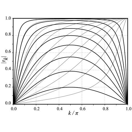
Figure 1: Bold lines: modulus of the single particle transmission coefficient $|\tau_{k}|$ through the weak link, see Eq. (14). From the top curve down: $t^{\prime}/t=0.1,0.2,\ldots,0.9$. Thin lines: the same quantity in the presence of a resonant state at the top of the single-particle band, see Eq. (18).

Determination of $T$ begins with calculating $G_{U}$ from Eqs. (8)-(10) using as input $\varepsilon_{k}=-2t\cos{k}$ and $U$ that has all the matrix elements zero except $u_{01}=u_{10}=t^{\prime}$. The translation-invariant part of $G_{U}$ can be obtained numerically by simply setting $t^{\prime}=0$. Alternatively, the two-particle spectral expansion yields for $G^{0}_{U}$ at $E<-4t$ the following expression [for the model (13), only $n_{1}=n_{2}$, $n^{\prime}_{1}=n^{\prime}_{2}$ matrix elements of $G^{0}_{U}$ are needed because of the locality of the Hubbard attraction]:

$$G^{0}_{U}( n,n ;n^{\prime},n^{\prime})$$ (16)

$$= \int^{\pi}_{-\pi}\!\!\!\int^{\pi}_{-\pi}\frac{dk_{1}dk_{2}}{(2\pi)^{2}}\frac{\cos{k_{1}(n-n^{\prime})}\cos{k_{2}(n-n^{\prime})}}{E+2t\cos{k_{1}}+2t\cos{k_{2}}}$$

$$= -\int^{\pi}_{-\pi}\frac{dq}{2\pi}\frac{\cos{q(n-n^{\prime})}}{\sqrt{E^{2}-8t^{2}-8t^{2}\cos{q}}}.$$

In accordance with the general scheme, the matrix $\delta G$ is calculated by subtracting $G^{0}_{U}$ from $G_{U}$. $\delta G(n,n^{\prime})$ is very localized around the weak link $n,n^{\prime}=0,1$, see Fig. 2.

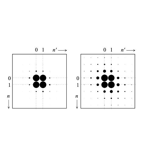
Figure 2: The non-translation invariant part of the Green operator $\delta G(n,n^{\prime})$ for $|v|=4.1\,t$ and $t^{\prime}=0.3\,t$. The pair momentum is $K=0.3\pi$ (left panel) and $K=0.8\pi$ (right panel). The radius of the circle represents the modulus $|\delta G|$. Notice the high degree of localization around the weak link.

The last thing we need is an expression for $B^{-1}$, see Eq. (12). Again, only the matrix elements in the block $n_{1}=n_{2}$ and $n^{\prime}_{1}=n^{\prime}_{2}$ are required. By diagonalizing the block by a Fourier transformation one can show that Bulatov1984 ; note

$$B^{-1}(n;n^{\prime})=\int^{\pi}_{-\pi}\frac{dq}{2\pi}\frac{\cos{q(n-n^{\prime})}}{1-\frac{|v|}{\sqrt{(E+i\gamma)^{2}-16t^{2}\cos^{2}(q/2)}}}.$$ (17)

Numerical results. The results obtained in the preceding section enable calculation of the full two-particle Green operator, the exact pair wave function, and the scattering coefficients of bound pairs for the model (13). In Fig. 3 we show the modulus $|\Psi_{K}|$ as a function of the particle coordinates $n_{1}$ and $n_{2}$ for $K=0.3\,\pi$, $|v|=4.1\,t$ and $t^{\prime}=0.3\,t$. Notice how reflection off the weak link creates interference between the incident and reflected wave functions. In contrast, the transmitted wave (in the lower right part of the graph) has a constant amplitude.

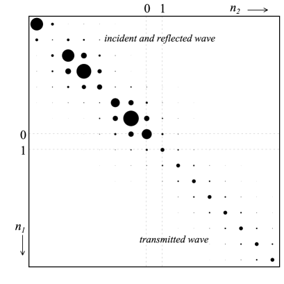
Figure 3: The pair wave function $\Psi_{K}(n_{1},n_{2})$ for $K=0.3\,\pi$, $|v|=4.1\,t$ and $t^{\prime}=0.3\,t$. The radius of the circle represents the modulus $|\Psi|$.

In Fig. 4 we show the pair transmission coefficient $T_{K}$. As a function of pair momentum, $T_{K}$ behaves qualitatively different from the one-particle transmission $\tau_{k}$, see Fig. 1. $\tau_{k}$ first increases with momentum but then decreases and vanishes at $k=\pi$. In contrast, $T_{K}$ is a monotonically increasing function of momentum, and reaches unity at $K=\pi$. Thus at large lattice momenta a bound pair is transmitted through a weak link much easier than a single particle. The likely physical reason for the anomalously high transmission is resonant tunneling through a two-body state localized at the weak link. Bulatov and Danilov BulDan1994 previously analyzed the two-particle spectrum of a semi-infinite Hubbard chain, i.e. model (13) with $t^{\prime}=t$. They found that the chain boundary introduces a resonant state with $E=-|v|$, i.e. exactly at the top edge of the pair band. We conjecture that such a state exists also at $t^{\prime}\neq t$ and facilitates efficient transmission through the weak link of pairs with energies close to the top of the band, i.e. with momenta close to $\pi$.

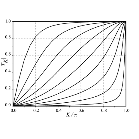
Figure 4: Pair transmission coefficient $T_{K}$ for $|v|=4.1$ and different $t^{\prime}/t$. From the top curve down: $t^{\prime}/t=0.1,0.2,\ldots,0.9$.

It is instructive to compare this effect with one-particle tunneling through the weak link in the presence of a resonant state. Such a state appears in the model (13) with $|v|=0$ if an additional one-particle repulsive potential $w$ is added at the two sites on either side of the weak link. At $w=t^{\prime}$, the state has the energy of the top of the one-particle band, $E=2t$. For those parameters, the transmission coefficient is note

$${\bar{\tau}}_{k}=\frac{(1-t^{\prime}/t)(e^{ik}-e^{-ik})}{(e^{ik}-e^{-ik})-2(t^{\prime}/t)(1+e^{ik})}.$$ (18)

This function is shown in Fig. 1 in thin lines. The resonant state qualitatively changes the transmission at large momenta. Instead of vanishing ${\bar{\tau}}_{k}$ actually approaches unity. The overall shape of the curves is remarkably similar to pair transmission curves of Fig. 4, which further supports our interpretation of pair tunneling as through a resonant state.

Summary. We have developed an efficient procedure of calculating scattering coefficients of bound pairs on a lattice. The key technical advance of the paper is the usage of two different decompositions of the hamiltonian; one is used to calculate the full Green operator of the system while another to find the resulting wave function of the pair. Another important element is the method of inverting the matrix $(1-G_{U}V)$, which is based on separating $G_{U}$ on a translation invariant part and a part localized around the scatterer, see Eqs. (11) and (12). The numerical accuracy of the method scales exponentially in the number of basis states chosen to represent the localized part. As formulated, the method is quite general enabling accurate investigation of a variety of scattering and tunneling problems. As the first application, we have studied transmission of bound pairs through a weak link on the one-dimensional chain. Contrary to simplistic expectations, we have found that at large momenta the pairs penetrate the barrier easier than single particles. The anomalously high transmission has been identified with tunneling through a resonant pair state. More two-body scattering problems are currently under investigation.

References

- (1) A.S. Davydov, Theory of Molecular Excitons (McGraw-Hill, New York, 1962).
- (2) R.S. Knox, Theory of Excitons (Academic, New York, 1963).
- (3) D. Mattis, The Theory of Magnetism (Springer, Berlin, 1981), Vol. 1.
- (4) S.A. Brazovskii and N.N. Kirova, Pis’ma Zh. Eksp. Teor. Fiz. 33, 6 (1981) [JETP Lett. 33, 4 (1981)].
- (5) A.J. Heeger, S. Kivelson, J.R. Schrieffer, and W.-P. Su, Rev. Mod. Phys. 60, 781 (1988).
- (6) R. Micnas, J. Ranninger, and S. Robaszkiewicz, Rev. Mod. Phys. 62, 113 (1990).
- (7) A.S. Alexandrov and N.F. Mott, High Temperature Superconductors and Other Superfluids (Taylor & Francis, 1994).
- (8) A.S. Alexandrov and P.E. Kornilovitch, J. Phys. Condens. Matter 14, 5337 (2002).
- (9) A.S. Davydov, Nonlinearity 2, 383 (1989).
- (10) D.C. Mattice, Rev. Mod. Phys. 58, 361 (1986).
- (11) P.A.F. da Viega, L. Ioriatti, and M. O’Carroll, Phys. Rev. E 66, 016130 (2002).
- (12) P.E. Kornilovitch, Phys. Rev. B 69, 235110 (2004).
- (13) S.L. Schwebel, Phys. Rev. 103, 814 (1956).
- (14) J.R. Jasperse and M.H. Friedman, Phys. Rev. 159, 69 (1967).
- (15) A.S. Alexandrov, A.M. Bratkovsky, and P.E. Kornilovitch, Phys. Rev. B 65, 155209 (2002).
- (16) V.V. Hizhnyakov, A.A. Maradudin, and D.L. Mills, Phys. Rev. B 11, 3149 (1975).
- (17) G. Gumbs and C. Mavroyannis, J. Phys. C: Solid State Phys. 14, 2199 (1981).
- (18) V.L. Bulatov, Fiz. Tverd. Tela 26, 2480 (1984) [Sov. Phys. Solid State 26, 1501 (1984)].
- (19) V.L. Bulatov, J. Phys. C: Solid State Phys. 20, 5421 (1987).
- (20) More details will be described elsewhere.
- (21) V.L. Bulatov and I.Yu. Danilov, Fiz. Tverd. Tela 36, 679 (1994) [Sov. Phys. Solid State 36, 373 (1994)].