Conduction electrons and the decoherence of impurity-bound electrons in a semiconductor

Abstract

We study the dynamics of impurity bound electrons interacting with a bath of conduction band electrons in a semiconductor. Only the exchange interaction is considered. We derive master equations for the density matrices of single and two qubit systems under the usual Born and Markov approximations. The bath mediated RKKY interaction in the two qubit case arises naturally. It leads to an energy shift significant only when the ratio ($R_{T}$) of the inter-qubit distance to the thermal deBroglie wavelength of the bath electrons is small. This bath mediated interaction also has a profound impact on the decoherence times; the effect decreases monotonically with $R_{T}$.

I introduction

The dynamics of the impurity bound electrons in semiconductors have been studied previously in the context of population relaxation Abrahams (1957); Pines et al. (1957); Honig (1954). Experimental studies of electron spin relaxation were central to understanding various mechanisms of relaxation of nuclear and electron spins in ³¹P atoms in Si. Since then, theoretical work has exhaustively considered the effects of various interactions among electrons and atoms on the relaxation of populations in different quantum states. Various researchers have considered the effects of spin-orbit coupling, hyperfine, exchange, Coulomb, and dipolar interactions. Current interest in the unusually long relaxation times predicted and observed in these systems stems from possible applications in solid-state quantum computing. The seminal proposal by Kane Kane (1998) to use ³¹P atoms embedded in Si crystal as qubits identifies one strategy for the realization of quantum computer hardware in the solid state.

Recent investigations of decoherence mechanisms in these schemes assume the presence of a strong magnetic field and low temperatures, typically, a few mK; this prevents spontaneous spin flips by breaking the degeneracy of bound electron spins Kane (1998); Hu and DasSarma (2003); Koiller et al. (2002); Loss and DiVincenzo (1998); deSousa and DasSarma (2003). The dominant decoherence mechanisms in this case include the hyperfine and dipolar interaction of electrons with nuclei, and dipolar-dipolar interaction among the electrons. Recent calculations Koiller et al. (2002); Hu and DasSarma (2003) suggest that at low temperatures decoherence is dominated by spin diffusion induced by hyperfine and dipolar interactions of qubits with the spin bath of Si atoms. In principle, and to a high degree in practice, this mechanism can be eliminated by using ultra pure ²⁸Si crystals. But it would be desirable to operate solid state quantum devices at low magnetic fields and higher temperatures, and the price for this is the importance of additional decoherence channels in the system. One of these is due to the interaction of qubits with a bath of conduction electrons. Studies of decoherence due to this channel have appeared in literature only recently Kim et al. (2004); Rikitake et al. (2004). The problem investigated by Kim et al. Kim et al. (2004) concerns the exchange interaction of a qubit with a spin polarized one dimensional stream of electrons. However, it only addresses the spin flip rates of the qubit, and uses a bath that is physically different from an unpolarized gas of conduction electrons typically found in a semiconductor. The latter type of bath is used by Rikitake et al. Rikitake et al. (2004) who study the effects of decoherence on the RKKY interaction of two qubits in a bath consisting of a non-interacting degenerate electron gas.

In this paper we consider a simple model, similar to that of Rikitake et al. Rikitake et al. (2004), in which the spins of electrons bound to donor atoms act as qubits and scatter the conduction electrons via the exchange interaction. For reasonably low donor densities, we show that the conduction electrons form a Boltzmann gas at all temperatures. Therefore, in a Kane type model only a classical distribution need be considered. The temperature is considered high enough that the ratio of bound to free electron density ensures that interactions among qubits are negligible compared to their exchange interaction with conduction electrons. For P atoms in Si, these assumptions are satisfied, in the absence of magnetic fields, for donor densities of the order of $10^{16}cm^{-3}$ or lower. The nature of the bath has important consequences for the temperature dependence of decoherence. Thus the results in the present paper are in contrast to those in of Rikitake et al., despite similar master equations obtained in both. Furthermore, the present paper addresses the Kane model more concretely and makes stronger connection between the parameters of the equations derived and fundamental properties of semiconductors.

In the following, we first present a full master equation for the density matrix of a single qubit and obtain an intuitive analytical result for the decoherence and relaxation times. The result is similar in form to the phenomenological result obtained by Pines et al.Pines et al. (1957) for the relaxation rates under conditions similar to those considered here. We then derive the master equation for a system of two mutually non-interacting qubits, and study the decoherence due to their interaction with the conduction electron bath. We plan to include the effects of interactions among qubits in a future paper.

II Model and Formal Equations

We consider a silicon lattice at nonzero temperatures doped with a density $n_{D}$ of phosphorus atoms. Each P atom donates an electron, which either becomes a conduction electron or is captured by another ionized P atom forming an “atom” with hydrogen-like properties. The captured electrons are usually in s-states with a “Bohr radius” of about 25 angstroms and a binding energy of about 0.044 eV deSousa and DasSarma (2003); Kohn and Luttinger (1955). The conduction electrons form a gas of approximately free particles with an effective mass of $0.2m_{e}$, where $m_{e}$ is the bare mass of the electron. The density of the gas builds up (from zero at $T=0$) as temperature rises and more donors are ionized. A simple statistical mechanics analysis shows that the expected number density of bound electrons at temperature $T$ is $n_{b}=n_{D}[1+\frac{1}{2}z^{-1}\exp(-E_{b}/k_{B}T)]^{-1}$, where $z$ is fugacity of the total system comprised of bound and unbound electrons, $E_{b}$ is the energy needed to excite a bound electron into the conduction band, and $k_{B}$ is Boltzmann’s constant. The conduction electron gas has a number density of

$$n_{c}(T) = 2\lambda_{T}^{-3}F_{3/2}(z),$$ (1)

where $F_{3/2}(z)=\int_{0}^{\infty}dx\sqrt{x}(z^{-1}e^{x}+1)^{-1}$ is the Fermi-Dirac function, and $\lambda_{T}=\hbar(2\pi/mk_{B}T)^{1/2}$ is the thermal deBroglie wavelength. Forcing $n_{c}+n_{b}=n_{D}$, we find

$$F_{3/2}(z)[2z+e^{-E_{b}/k_{B}T}] = \frac{1}{2}n_{D}\lambda_{T}^{3}e^{-E_{b}/k_{B}T}.$$ (2)

For the parameters chosen, the product $\lambda_{T}^{3}e^{-E_{b}/k_{B}T}<10^{-24}cm^{3}$ for temperatures below 300 K, which implies that for $n_{D}\approx 10^{16}cm^{-3}$, we can take $z\ll 1$ and $F_{3/2}(z)\approx z$ . Consequently, the distribution of conduction electron gas remains Boltzmann down to $T=0$.

We simplify the picture by assuming the qubits to be in s-states, with only the spin acting as their degree of freedom, and suppose there are no external fields breaking the degeneracy of the spin states. The conduction electrons collide occasionally with the qubits elastically; we assume they do not excite them into higher states. However, the spins of the two may become entangled or even exchanged. Since the conduction electron moves throughout the crystal interacting with many electrons and atoms before the qubit scatters another conduction electron, it loses its coherence much faster than the qubits, and may be thought to be in an incoherent superposition of momentum eigenstates over the timescale of interest. Thus it is also independent of other bath electrons, while being on the same footing as them. This allows us to study only the case of interaction between a qubit and one mixed state conduction electron, and multiply by the number of the latter in the end result. Thus we can take our Hamiltonian as

$$H = \frac{\mathbf{p}^{2}}{2m}+V,$$ (3)

where p is the momentum of the conduction electron and $m$ is its effective mass. The operator $V$ is the interaction Hamiltonian acting on the electron and the qubit(s). We are concerned only with the exchange interaction, and study two cases. We first consider a single qubit at the origin for which the interaction takes the form

$$V = Jr_{0}^{3}\delta(\mathbf{r})\mathbf{S}\cdot\mathbf{s},$$ (4)

where $J$ is the exchange coefficient and $r_{0}$ is an effective Bohr radius characterizing the size of the qubit. The spin operators $\mathbf{S}$ and s act on the qubit and the conduction electrons respectively. We also consider two mutually non-interacting qubits for which the interaction is

$$V = Jr_{0}^{3}\left[\delta(\mathbf{r}-\frac{1}{2}\mathbf{R})\mathbf{S}_{1}\cdot\mathbf{s}+\delta(\mathbf{r}+\frac{1}{2}\mathbf{R})\mathbf{S}_{2}\cdot\mathbf{s}\right],$$ (5)

where $\mathbf{S}_{1}$ and $\mathbf{S}_{2}$ are the qubit spin operators, and the two qubits are placed symmetrically at $\pm\mathbf{R}/2$. To treat more than two qubits, similar terms would be added to $V$, with delta functions centered at the respective qubit locations. Despite the absence of direct exchange interaction between them, the two qubits can still exchange spins via indirect exchange interaction. Physically this occurs when the bath remains correlated long enough for the conduction electron to link two qubits; the indirect exchange coupling between qubits can arise even when they are too far away to have significant direct exchange interaction. This coupling is significant only when the inter-qubit distance is much shorter than the coherence length of the bath, which is approximately the thermal deBroglie wavelength $\lambda_{T}$. The results found here depend naturally on these two important length scales.

In addition, there are also direct interactions between the qubits. The important qubit-qubit interactions involve the exchange interaction between bound electrons, the hyperfine, dipolar, and spin-orbit coupling of these electrons to the bath of Si nuclei. For low doping densities the first of these can be ignored as a starting point. For a donor density of $n_{D}=10^{16}cm^{-3}$, and $T=100K$, the inter-donor distance is $R\approx 50$ nm, whereas the mean radius of the electron orbits is $r_{0}\approx 2.5$ nm. Thus the exchange energy is small, as we expect little overlap between the qubit wave functions. The second and third have been studied by various authors in the context of both relaxation and decoherence rates Abrahams (1957); Pines et al. (1957); Feher et al. (1955); Honig (1954); Tyryshkin et al. (2003); Koiller et al. (2002); Hu and DasSarma (2003). The hyperfine and dipolar terms can be made arbitrarily small by purifying the Si samples to contain only the ²⁸Si isotope. For natural Si, which contains 95.33% ²⁸Si, it is estimated that the hyperfine and dipolar couplings combined are of the order of $10^{-7}$ eV or less deSousa and DasSarma (2003). This is minute compared to the exchange interaction on the order of meV that we consider. Spin-orbit coupling is likewise small, and we neglect these additional effects in this preliminary investigation.

We point out that the model has important differences to the one used by Chang et al. in their general study of dissipative dynamics of a two-state systemL.D. Chang (1984). They consider a biased qubit that is coupled to the bath via $S_{z}$ only, and the coupling induces no spin-flips in either the bath or the qubit. Furthermore, spin flips are introduced by a tunneling parameter that is independent of the bath state. This is clearly not the case in (4-5) where the isotropic coupling of system and bath causes joint spin flips in the two subsystems. A more general case of Brownian motion in a fermionic environment has also been studied in several papers by ChenChen (1987a, b, c), who mainly focused on mapping between fermionic and bosonic environments. None of these studies discusses decoherence directly, and it is highly nontrivial to extend the results of these papers to arrive at those in this work.

We first develop a general equation for the density matrix $\rho(t)$ of a system coupled to a bath and the full system evolving via the Hamiltonian in (3). The following notation is used. We label the conduction electron states by $\left|\alpha\mathbf{p}\right\rangle=\left|\alpha\right\rangle\otimes\left|\mathbf{p}\right\rangle$, where $\left|\alpha\right\rangle$ and $\left|\mathbf{p}\right\rangle$ are the eigenstates of $s^{z}$ and the momentum operator of the conduction electron respectively. The kinetic energy of the bath electron is denoted by $\hbar\omega_{p}=p^{2}/2m$, and the normalized system states are labelled using Roman letters. For a general interaction $V$, we write the interaction Hamiltonian in the interaction picture as

$$H_{I}(t) = \sum_{ij}\left|i\right\rangle\left\langle j\right|\otimes\sum_{\alpha,\alpha^{\prime}}\sum_{\mathbf{p},\mathbf{p}^{\prime}}e^{i(\omega_{p}-\omega_{p^{\prime}})t}\left|\alpha\mathbf{p}\right\rangle\left\langle\alpha\mathbf{p}\right|V_{ij}\left|\alpha^{\prime}\mathbf{p}^{\prime}\right\rangle\left\langle\alpha^{\prime}\mathbf{p}^{\prime}\right|$$ (6)

Here we defined bath operators $V_{ij}=\left\langle i\right|V\left|j\right\rangle$ which depend parametrically on system states. It is shown in the Appendix that for an unpolarized bath under the Born approximation, the density matrix $\rho$ of the system is given by

$$\dot{\rho} = -i\omega_{RKKY}\sum_{ijkl}\Gamma_{ijkl}[\eta_{ij}\eta_{kl},\rho]+\gamma\sum_{ijkl}\Lambda_{ijkl}(2\eta_{kl}\rho\eta_{ij}-\eta_{ij}\eta_{kl}\rho-\rho\eta_{ij}\eta_{kl}),$$ (7)

where the operators $\eta_{ij}=\left|i\right\rangle\left\langle j\right|$ are system operators. The tensors $\Gamma$ and $\Lambda$, and the constants $\gamma$ and $\omega_{RKKY}$, result from specializing (48) and (52) to the two the forms of $V$ shown in (4) and (5). It is evident that $\Gamma$ is involved with a unitary evolution of $\rho(t)$ and $\Lambda$ with the decoherence processes. Thus we label the first sum as the unitary term and the second as the dissipative or non-unitary. The frequency $\omega_{RKKY}$ is a shift resulting from the RKKY interaction between the two qubits. No such term arises in the single qubit problem. The constant $\gamma^{-1}$ is an interaction time constant of the system and the bath, (see appendix for derivation); $\gamma$ and $\omega_{RKKY}$ are defined as

$$\gamma = 4(2\pi)^{-\frac{3}{2}}n_{c}(T)(Jr_{0}^{3}m\hbar^{-2})^{2}\sqrt{\frac{k_{B}T}{m}},$$ (8)

$$\omega_{RKKY}(\mathbf{R}) = -(2\pi)^{3}\hbar^{-1}(Jr_{0}^{3})^{2}\chi(\mathbf{R})$$ (9)

$$= \frac{4}{\pi}n_{c}(T)(Jr_{0}^{3}m\hbar^{-2})^{2}\frac{\hbar}{mR}e^{-\pi(2R/\lambda_{T})^{2}}.$$ (10)

In the definition (9) of $\omega_{RKKY}$, $\chi(\mathbf{r})$ is the free electron susceptibility, and the expression in (10) specializes this definition to a Boltzmann distribution for the conduction electron gas. Apart from dimensionless factors, $\gamma$ is a product of the thermal flux of conduction electrons and an “effective area” $(Jr_{0}^{3}m\hbar^{-2})^{2}$ over which the bound electron experiences this flux. On the other hand, the thermal flux in the definition of $\omega_{RKKY}$ is replaced by $n_{c}\hbar(mR)^{-1}\exp(-4\pi R_{T}^{2})$, which depends on the inter-qubit distance and the thermal deBroglie wavelength of bath electrons. Both these rates are given by a mean number of scattering events, where the scattering occurs via the exchange interaction. The $1/R$ divergence of $\omega_{RKKY}$ is typical of the $\chi(\mathbf{r})$ in three dimensions Larsen (1981); Kim et al. (1995) but the spatial damping factor in the case of Boltzmann distribution is Gaussian as opposed to exponential in the degenerate limit Kim et al. (1995). Furthermore, the increase in decoherence with $n_{c}$ and $J$ is accompanied by a correspondingly faster unitary evolution, as the ratio $\gamma^{-1}\omega_{RKKY}$ is independent of both these parameters.

III Application to two specific cases

III.1 Dynamics of a single qubit

This is the simplest application of the general expressions given above, and we use it to estimate the temperature dependence of relaxation and decoherence times. The tensors $\Gamma$ and $\Lambda$ in this case are equal and their tensor elements are found to be

$$\Lambda_{ijkl} = \frac{1}{2}\left\langle i\right|S^{z}\left|j\right\rangle\left\langle k\right|S^{z}\left|l\right\rangle+\frac{1}{4}\left\langle i\right|S^{+}\left|j\right\rangle\left\langle k\right|S^{-}\left|l\right\rangle+\frac{1}{4}\left\langle i\right|S^{-}\left|j\right\rangle\left\langle k\right|S^{+}\left|l\right\rangle,$$ (11)

where $S^{\pm}=S^{x}\pm iS^{y}$. Substitution of this expression in (7) yields the master equation for a single qubit explicitly in the Lindblad form. The unitary term becomes $[S^{2},\rho]$, and it vanishes because $S^{2}$ is proportional to identity. We define a superoperator $\mathcal{L}(.)$ such that $\mathcal{L}(A)\rho=2A\rho A^{\dagger}-A^{\dagger}A\rho-\rho A^{\dagger}A$, where $A$ is a general operator, and obtain

$$\dot{\rho} = \frac{\gamma}{2}[\mathcal{L}(S^{x})\rho+\mathcal{L}(S^{y})\rho+\mathcal{L}(S^{z})\rho]$$ (12)

$$= -\frac{\gamma}{2}([S^{x},[S^{x},\rho]]+[S^{y},[S^{y},\rho]]+[S^{z},[S^{z},\rho]]).$$ (13)

The latter equality follows due to the Hermiticity of the spin operators. Besides ensuring complete positivity and trace preservation, this form is also invariant under arbitrary rotations of the spin. Therefore we may consider any pure initial state to be a spin up state in the $S^{z}$ basis of a suitable coordinate frame. In the Bloch formalism, these states reside on the surface of a unit sphere and their loss of purity is described by the decay in the length of the vector representing them. From (13) we then find that the initial decay of purity is equal to $d\mathsf{Tr}[\rho^{2}]/dt=-\gamma$ for all pure states.

To study the evolution of a general state, we study the Bloch vector with components $u=\rho_{01}+\rho_{10}$, $v=i(\rho_{01}-\rho_{10})$, and $w=\rho_{11}-\rho_{00}$. Here 0 identifies the “spin down” state and 1 the “spin up” state. From the master equation (13) it follows that

$$\dot{u} = -\gamma u,\,\,\,\dot{v}=-\gamma v,\,\,\,\dot{w}=-\gamma w.$$ (14)

From these equations we find that the longitudinal and transverse rates are $T_{1}^{-1}=T_{2}^{-1}=\gamma$. Thus the relaxation rate is proportional to the collision rate of a qubit with a thermalized bath of particles. The two rates are equal because the system is unbiased, and both relaxation and decoherence arise only through elastic scattering. The conventional relation $2T_{2}\leq T_{1}$ holds true only when several distinct scattering processes determine $T_{2}$ while only a subset of them is responsible for $T_{1}$. When no such distinction exists we can have $T_{1}=T_{2}$ , as Bloch noted many years ago Bloch (1946).

In Si:P with physical parameters defined in Section II, we estimate $J\approx 6$meV. Taking into account the temperature dependence of $n_{c}(T)$, shown in Figure (1), we plot $\log(\gamma^{-1})$ as a function of $T$ in Figure (2) (the logarithm base is 10). It is evident from the figure that above about 70 K, $\gamma^{-1}$ is less than a microsecond, which means that conduction electrons present a significant decoherence mechanism in this regime. The effectiveness of this channel vanishes significantly at low temperatures due to the loss of conduction electrons (as discussed in Section II); $n_{c}$ is less than 1 percent of $n_{D}$ for $T<35$K. The $\sqrt{T}$ dependence of the thermal flux, which is associated with a decrease in conduction electron velocity with lowering temperature, also contributes to the rapid decrease in $\gamma$ as temperature is decreased.

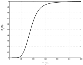
Figure 1: Ratio of conduction electron density to donor density as a function of temperature

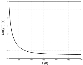
Figure 2: Decoherence time for a single qubit as a function of temperature (logarithm base 10).

III.2 Dynamics of two mutually non-interacting qubits

We now consider a system of two mutually non-interacting qubits that relax and decohere via the exchange interaction with the conduction electrons. Again, the general dynamical map (7) describes the evolution upon specializing the tensors $\Lambda$ and $\Gamma$ to (5) using the defining equations (48) and (52). As expected a contribution of the form (11) for a single qubit comes from each member of the system. We call this $\Lambda^{\prime}$ and write it as

$$\Lambda^{\prime}_{ijkl} = \sum_{q=1}^{2}\frac{1}{2}\left\langle i\right|S_{q}^{z}\left|j\right\rangle\left\langle k\right|S_{q}^{z}\left|l\right\rangle+\frac{1}{4}\left\langle i\right|S_{q}^{+}\left|j\right\rangle\left\langle k\right|S_{q}^{-}\left|l\right\rangle+\frac{1}{4}\left\langle i\right|S_{q}^{-}\left|j\right\rangle\left\langle k\right|S_{q}^{+}\left|l\right\rangle,$$ (15)

where $q=1,2$ labels each qubit. However, there also exist “cross-coupling” terms which represent the process by which a conduction electron mediates a spin exchange between the two qubits. These are given by $\Lambda^{\prime\prime}$ where

$$\Lambda^{\prime\prime}_{ijkl} = \frac{1}{2}\left\langle i\right|S_{1}^{z}\left|j\right\rangle\left\langle k\right|S_{2}^{z}\left|l\right\rangle+\frac{1}{4}\left\langle i\right|S_{1}^{+}\left|j\right\rangle\left\langle k\right|S_{2}^{-}\left|l\right\rangle+\frac{1}{4}\left\langle i\right|S_{1}^{-}\left|j\right\rangle\left\langle k\right|S_{2}^{+}\left|l\right\rangle$$ (16)

$$+\frac{1}{2}\left\langle i\right|S_{2}^{z}\left|j\right\rangle\left\langle k\right|S_{1}^{z}\left|l\right\rangle+\frac{1}{4}\left\langle i\right|S_{2}^{+}\left|j\right\rangle\left\langle k\right|S_{1}^{-}\left|l\right\rangle+\frac{1}{4}\left\langle i\right|S_{2}^{-}\left|j\right\rangle\left\langle k\right|S_{1}^{+}\left|l\right\rangle.$$

The two tensors add to form the tensors that appear in (7):

$$\Lambda_{ijkl} = \Lambda^{\prime}_{ijkl}+\xi(R_{T})\Lambda^{\prime\prime}_{ijkl},$$ (17)

$$\Gamma_{ijkl} = \Lambda^{\prime\prime}_{ijkl},$$ (18)

$$\xi(R_{T}) = \int_{0}^{\infty}xe^{-x}\mathrm{sinc}^{2}[R_{T}\sqrt{4\pi x}]dx=\frac{-i\mathrm{Erf}(iR_{T}\sqrt{4\pi})}{4R_{T}}e^{-4\pi R^{2}_{T}}$$ (19)

where $R_{T}=R/\lambda_{T}$ is the inter-qubit distance measured in units of the thermal deBroglie wavelength, and $\mathrm{Erf}(.)$ denotes the error function. The tensor $\Gamma$ depends only on $\Lambda^{\prime\prime}$ because the term corresponding to $\Lambda^{\prime}$ commutes with $\rho(t)$, as can be verified from (7). The dimensionless integral $\xi(R_{T})$ represents the strength of indirect exchange coupling between the two qubits relative to their direct exchange interaction with the conduction electrons. The most dominant contribution to the integral comes from $x<\pi/4R_{T}^{2}$. Thus we find, as expected, that the strength of indirect exchange decreases rapidly as qubits move out of the coherence region of the conduction electron, and the plot of $\xi(R_{T})$ in Figure (3) shows a monotonic decrease as $R_{T}$ increases. We point out that if the Fermi distribution were applicable, $\xi(R,T)$ would be given by the same formula as above, but with $xe^{-x}$ replaced by the $x(z^{-1}e^{x}+1)^{-1}$, where $z$ is the fugacity of the gas. At vanishingly small temperatures, the Fermi wavelength would then take the role of the thermal deBroglie wavelength in setting the length-scale of indirect exchange. But we stress that for the model presented in section II the Boltzmann distribution is relevant for all temperatures.

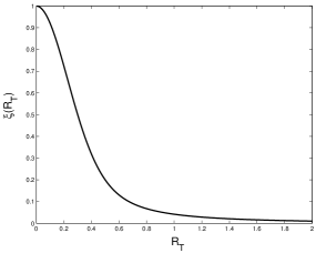
Figure 3: $\xi(R_{T})$ as a function of $R_{T}=R/\lambda_{T}$

Complete positivity and trace preservation is guaranteed in the two qubit case as well. Substitution of (15-16) in (7) yields

$$\dot{\rho} = -\frac{i}{\hbar}[H_{eff},\rho]+\sum_{k,l=1}^{6}c_{kl}[2F_{k}\rho F_{l}^{\dagger}-\{F_{l}^{\dagger}F_{k},\rho\}],$$ (20)

where we have defined an effective Hamiltonian

$$H_{eff} = \hbar\omega_{RKKY}\mathbf{S}_{1}\cdot\mathbf{S}_{2},$$ (21)

which causes unitary evolution due to system bath interaction. The dissipative part contains six operators $(F_{1},F_{2},F_{3},F_{4},F_{5},F_{6})=(S_{1}^{z},S_{1}^{+},S_{1}^{-},S_{2}^{z},S_{2}^{+},S_{2}^{-})$, and a $6\times 6$ symmetric coefficient matrix

$$c = \,\,\left[\begin{array}[]{cc}a&\xi a\\ \xi a&a\end{array}\right],$$ (24)

$$a = \frac{1}{4}\left[\begin{array}[]{ccc}2&0&0\\ 0&1&0\\ 0&0&1\end{array}\right].$$ (28)

The matrix $c$ is positive semidefinite, as can be verified from its non-negative eigenvalues for $0\leq\xi\leq 1$. This is sufficient to ensure complete positivity of (20). The equation is reduced to Lindblad form by diagonalizing $c$ and obtaining an orthonormal set of eigenvectors. Thus

$$\dot{\rho} = -\frac{i}{\hbar}[H_{eff},\rho]$$ (29)

$$+\frac{1}{4}\gamma(1+\xi)[\mathcal{L}(S_{2}^{x}+S_{1}^{x})+\mathcal{L}(S_{2}^{y}+S_{1}^{y})+\mathcal{L}(S_{2}^{z}+S_{1}^{z})]\rho$$

$$+\frac{1}{4}\gamma(1-\xi)[\mathcal{L}(S_{2}^{x}-S_{1}^{x})+\mathcal{L}(S_{2}^{y}-S_{1}^{y})+\mathcal{L}(S_{2}^{z}-S_{1}^{z})]\rho.$$

An equation of the same form has been derived by Rikitake et al. but with the parameters specific to a degenerate bathRikitake et al. (2004). Let us now compare this map with the single qubit map (12) by ignoring the unitary term. For the case $\xi=0$, $c$ is already diagonal, and the spin operators of each qubit form the set of Lindblad operators in the dynamical map. The map then consists of a sum of maps (12) for each qubit, which implies that the reduced dynamics of each qubit is independent of the other. Physically, at $\xi=0$, the coherence length of the bath is much smaller than the inter-qubit distance, and therefore the qubits scatter bath electrons independently of each other.

In the presence of indirect coupling, the Lindblad operators are not the spin operators of the qubits but their sum $\mathbf{S}=\mathbf{S}_{2}+\mathbf{S}_{1}$, and difference $\mathbf{\Delta}=\mathbf{S}_{2}-\mathbf{S}_{1}$. For significant values of $\xi$, the coherence length of the bath covers the inter-qubit distance. When scattering the bath electrons, it is then reasonable to expect that the two qubits behave as a single entity with total spin $\mathbf{S}$. In fact, in the extreme limit of full coherence over the region containing the qubits, $\xi=1$, and the map has exactly the same form as that of the single qubit map. The difference operator, $\mathbf{\Delta}$, accounts for the deviation from perfect coherence of conduction electrons at the two sites, and allows independent evolution to take place; the magnitude of this effect is of order $1-\xi$. This suggests that the singlet state with a total spin zero should be free of dissipative dynamics whenever $\xi=1$, and this is found to be the case in the solution of (29) presented below. Note that this is true not just within the context of the Born approximation to the scattering amplitudes. Since $\xi=1$ strictly only for $\mathbf{R}=0$ (it is meaningless to consider $T=0$ as $n_{c}(0)=0$), the interaction becomes $V=J\delta(\mathbf{r})\mathbf{s}\cdot\mathbf{S}$. The operator $\mathbf{S}$ has a nullspace with the singlet as its only member, and therefore, the singlet stops interacting with the bath when $\xi=1$, and remains pure indefinitely. More generally, the purity is clearly long lived whenever $\lambda_{T}\gg R$, and $\xi\approx 1$. Note also that no state other than the singlet can be in isolation because a nonzero total spin would always interact with the bath electrons. Finally, the dynamics of the singlet was briefly considered by Rikitake et al.. They find similar behavior for the singlet, but where the thermal deBroglie wavelength is replaced by Fermi wavelength, as was pointed out earlier for the case of a degenerate gas.

Let us now consider in detail a realistic case of intermediate values of $\xi$. In order to proceed, we analytically solve (29), which is done most conveniently in the Bell-basis representation of $\rho(t)$, where the basis vectors are enumerated in the order they are shown below:

$$\left\{\frac{\left|00\right\rangle+\left|11\right\rangle}{\sqrt{2}},\,\,\frac{\left|00\right\rangle-\left|11\right\rangle}{\sqrt{2}},\,\,\frac{\left|01\right\rangle+\left|10\right\rangle}{\sqrt{2}},\,\,\frac{\left|01\right\rangle-\left|10\right\rangle}{\sqrt{2}}\right\}.$$

The first (second) symbol corresponds to the first (second) qubit. In this basis the operators $\mathbf{S}$ and $\mathbf{\Delta}$ take a particularly simple form as shown in Table (1). It is evident from the table and (29) that the diagonal terms of the density matrix do not couple to the off-diagonal ones. This simplifies the calculation and yields the following population equations:

$$\frac{d}{dt}(\rho_{22}-\rho_{11}) = -\gamma(2+\xi)(\rho_{22}-\rho_{11}),$$ (30)

$$\frac{d}{dt}(\rho_{33}-\rho_{11}) = -\gamma(2+\xi)(\rho_{33}-\rho_{11}),$$ (31)

$$\frac{d}{dt}\sum_{i=1,2,3}\rho_{ii} = -2\gamma(1-\xi)\sum_{i=1,2,3}\rho_{ii}+\frac{3\gamma}{2}(1-\xi)$$ (32)

$$\frac{d}{dt}\rho_{44} = -2\gamma(1-\xi)\rho_{44}+\frac{\gamma}{2}(1-\xi).$$ (33)

The first two equations show that the populations within the triplet manifold equilibrate to a uniform distribution at a rate of $\gamma(2+\xi)$. The last two show that the population transfer between this and the singlet manifold occurs at a rate of $2\gamma(1-\xi)$, confirming our observation that the singlet ceases to evolve at $\xi=1$. The off-diagonal elements couple only to their conjugates. Within the triplet manifold they obey

$$\rho_{12}(t) = \left(\Re[\rho_{12}(0)]+i\Im[\rho_{12}(0)]e^{-\gamma(1+\xi)t}\right)e^{-\gamma t},$$ (34)

$$\rho_{13}(t) = \left(\Re[\rho_{13}(0)]+i\Im[\rho_{13}(0)]e^{-\gamma(1+\xi)t}\right)e^{-\gamma t},$$ (35)

$$\rho_{23}(t) = \left(\Re[\rho_{23}(0)]e^{-\gamma(1+\xi)t}+i\Im[\rho_{23}(0)]\right)e^{-\gamma t},$$ (36)

while the elements between the triplet and the singlet manifolds obey

$$\rho_{14}(t) = \Re[\rho_{14}(0)]\left\{\cos(\omega^{\prime}t)-(i\omega+\gamma^{\prime})\frac{\sin(\omega^{\prime}t)}{\omega^{\prime}}\right\}e^{-\gamma(3-\xi)t/2}$$ (37)

$$+i\Im[\rho_{14}(0)]\left\{\cos(\omega^{\prime}t)-(i\omega-\gamma^{\prime})\frac{\sin(\omega^{\prime}t)}{\omega^{\prime}}\right\}e^{-\gamma(3-\xi)t/2},$$

$$\rho_{24}(t) = \Re[\rho_{24}(0)]\left\{\cos(\omega^{\prime}t)-(i\omega-\gamma^{\prime})\frac{\sin(\omega^{\prime}t)}{\omega^{\prime}}\right\}e^{-\gamma(3-\xi)t/2}$$ (38)

$$+i\Im[\rho_{24}(0)]\left\{\cos(\omega^{\prime}t)-(i\omega+\gamma^{\prime})\frac{\sin(\omega^{\prime}t)}{\omega^{\prime}}\right\}e^{-\gamma(3-\xi)t/2},$$

$$\rho_{34}(t) = \Re[\rho_{34}(0)]\left\{\cos(\omega^{\prime}t)-(i\omega-\gamma^{\prime})\frac{\sin(\omega^{\prime}t)}{\omega^{\prime}}\right\}e^{-\gamma(3-\xi)t/2}$$ (39)

$$+i\Im[\rho_{34}(0)]\left\{\cos(\omega^{\prime}t)-(i\omega+\gamma^{\prime})\frac{\sin(\omega^{\prime}t)}{\omega^{\prime}}\right\}e^{-\gamma(3-\xi)t/2}.$$

Here we defined the difference of eigenvalues of $H_{eff}$ in the triplet and singlet manifolds as $\hbar\omega=\left\langle k\right|H_{eff}\left|k\right\rangle-\left\langle 4\right|H_{eff}\left|4\right\rangle$ , where $k=1,2$ or $3$ labels the triplet states. The renormalized frequency $\omega^{\prime}=\sqrt{\omega^{2}-\gamma^{\prime 2}}$, where $\gamma^{\prime}=\gamma(1-\xi)/2$, represents the oscillations caused by the unitary evolution resulting from the RKKY interaction. It follows from Table (1) that these oscillations are absent within the triplet manifold; they also disappear for $\omega<\gamma^{\prime}$ in the above equations. We note that the off-diagonal elements always decay at least with a rate of $\gamma$, and each of these elements is uncoupled from all others. Hence dephasing between any pair of Bell states proceeds independently of the rest of the states.

Table 1: Bell basis representation of the spin operators $\mathbf{S}$ and $\mathbf{\Delta}$.

$j\rightarrow$	$x$	$y$	$z$
$S^{j}$	$\left|1\right\rangle\left\langle 3\right|+\left|3\right\rangle\left\langle 1\right|$	$-i\left|2\right\rangle\left\langle 3\right|+i\left|3\right\rangle\left\langle 2\right|$	$\left|1\right\rangle\left\langle 2\right|+\left|2\right\rangle\left\langle 1\right|$
$\Delta^{j}$	$-\left|2\right\rangle\left\langle 4\right|-\left|4\right\rangle\left\langle 2\right|$	$-i\left|1\right\rangle\left\langle 4\right|+i\left|4\right\rangle\left\langle 1\right|$	$\left|3\right\rangle\left\langle 4\right|+\left|4\right\rangle\left\langle 3\right|$

Equations (30-33) show that, for $\xi\neq 1$, the final state of the density matrix is the maximum entropy state $\rho=\frac{1}{4}\mathbf{1}$. However, for $\xi=1$, the relaxation between the singlet state and the triplet manifold ceases, and the final state becomes $\rho_{44}^{final}=\rho_{44}(0)$ and $\rho_{ii}^{final}=\frac{1}{3}(1-\rho_{44}(0))$ for $i=1,2,3$. The relaxation rate of the singlet can become zero, but all other states attain a minimum relaxation rate of $2\gamma$.

Several other properties of the dynamical map (29) become evident when we consider the rate of decrease in purity of an initially pure state; the map ensures that the purity $p(t)=\mathsf{Tr}[\rho^{2}(t)]$ is a monotonically decreasing function of time. A general equation for the rate of change of purity follows straightforwardly from (29) as

$$\frac{dp}{dt} = -3\gamma(1-\xi)p-2\gamma\xi\mathsf{Tr}[S^{2}\rho^{2}]+\gamma\mathsf{Tr}\left[(1+\xi)(\mathbf{S}\rho)\cdot(\mathbf{S}\rho)+(1-\xi)(\mathbf{\Delta}\rho)\cdot(\mathbf{\Delta}\rho)\right].$$ (40)

For pure initial states $\rho(0)=\left|\psi\right\rangle\left\langle\psi\right|$, the initial loss in purity occurs at the rate

$$\dot{p}(0) = -3\gamma(1-\xi)-2\gamma\xi\left\langle\psi\right|S^{2}\left|\psi\right\rangle+\gamma(1+\xi)\left\|\left\langle\psi\right|\mathbf{S}\left|\psi\right\rangle\right\|^{2}+\gamma(1-\xi)\left\|\left\langle\psi\right|\mathbf{\Delta}\left|\psi\right\rangle\right\|^{2}.$$ (41)

It is easily verified that the separable states of the general form $\left|a\right\rangle\left|b\right\rangle$ lose initial purity at the rate $\dot{p}(0)=\gamma(-3+2\left\|\left\langle a\right|\mathbf{S}_{1}\left|a\right\rangle\right\|^{2}+2\left\|\left\langle b\right|\mathbf{S}_{2}\left|b\right\rangle\right\|^{2})$, which is independent of $\xi$. Thus the size of $\xi$ has no effect on the initial decay in purity of unentangled states. Furthermore, since any state corresponds to “spin up” in some direction, we have $\left\langle a\right|\mathbf{S}_{1}\left|a\right\rangle\cdot\left\langle a\right|\mathbf{S}_{1}\left|a\right\rangle=\left\langle b\right|\mathbf{S}_{2}\left|b\right\rangle\cdot\left\langle b\right|\mathbf{S}_{2}\left|b\right\rangle=1/4$, and all separable states are on an equal footing with respect to the initial rate of loss in purity.

We now show that this is in fact the minimum rate achievable within the triplet manifold. An arbitrary state in the triplet manifold has $\left\langle\psi\right|S^{2}\left|\psi\right\rangle=2$, and $\left\langle\psi\right|\mathbf{\Delta}\left|\psi\right\rangle=0$, which when substituted in (41) yields the initial rate $\dot{p}(0)=-\gamma(3+\xi-(1+\xi)\left\|\left\langle\psi\right|\mathbf{S}\left|\psi\right\rangle\right\|^{2})$ with only one state dependent variable, $\left\|\left\langle\psi\right|\mathbf{S}\left|\psi\right\rangle\right\|$. The maximum value of $\left\|\left\langle\psi\right|\mathbf{S}\left|\psi\right\rangle\right\|$ occurs for a separable $\psi$, which consists of parallel spins. Therefore, we see that within the triplet manifold, separable states are the most robust against loss in purity.

On the other hand, the singlet has $|\dot{p}(0)|=3\gamma(1-\xi)$, which becomes less than $2\gamma$ for $\xi>1/3$. Therefore the singlet is more robust than the separable-states in this regime. The rate corresponding to any superposition of singlet and separable states is greater than the average of the rates of these states. Consequently, the set of robust states does not change in any continuous manner with $\xi$, and it instead changes from separable to singlet at $\xi=1/3$. For $t>0$, the fidelity, $f(t)\equiv\mathsf{Tr}[\rho(t)\rho(0)]$, offers a characterization for predictability in which $f(t)\approx 1$ identifies a highly predicable state and $f(t)\approx 0$ a poorly predicable one. In a study of fidelity, not reported here, we found that the set of most predicable states makes a transition from separable to singlet state for $1/3<\xi<1/2$, depending on the time elapsed.

We end this section by discussing the time-dependent behavior of $\dot{p}(t)$ for a few simple cases. Since for our Hilbert space of dimension 4, $p(t)$ decreases monotonically to the value $1/4$ for $\xi\neq 1$, it is useful to define an “instantaneous rate” for purity

$$a(t) = -\frac{\dot{p}}{p-0.25},$$

in terms of which

$$p(t) = \frac{1}{4}+\frac{3}{4}\exp\left(-\int_{0}^{t}a(t^{\prime})dt^{\prime}\right).$$

The function $a(t)$ highlights differences in $\dot{p}(t)$, and it is especially useful when different states lead to similar behavior for $\dot{p}(t)$. We first consider the separable states of the form

$$\left|\psi\right\rangle = \left|0\right\rangle(\cos(\phi)\left|0\right\rangle+\sin(\phi)\left|1\right\rangle)$$

and plot the $\phi$-parameterized rate $a_{\phi}(t)$ as a function of $\phi$ and time $t$ for different values of $\xi$. Figure (4a) shows that all separable states give rise to exactly the same rate at all times for $\xi=0$. Here we set $\omega=0$ to describe the effects of non-unitary dynamics only. The effect of non-zero exchange coupling becomes evident in Figure (4b) where we set $\xi=0.7$. Here the function $a_{\phi}(t)$ decays much more slowly with time for states $\phi\approx\pi/4$ than for $\phi\in\{0,\pi/2\}$. Thus while $\xi$ plays no role initially for the separable states, the more stable states are those with both qubits prepared parallel or anti-parallel to each other (see discussion after (41)). Similarly, the most vulnerable of separable states are those in which the qubits are eigenstates of spin operators corresponding to orthogonal Cartesian directions.

The purity of the four Bell states has the following time dependence:

$$p_{i}(t) = \frac{1}{4}+\frac{1}{12}e^{-4\gamma(1-\xi)t}+\frac{2}{3}e^{-2\gamma(2+\xi)t},\,\,\,\,i=1,2,3$$

$$p_{4}(t) = \frac{1}{4}+\frac{3}{4}e^{-4\gamma(1-\xi)t}.$$

Thus the three states with total spin $S\neq 0$ lose purity for all values of $\xi$, and do so at two different rates for $\xi\neq 1$. Initially, the decay is dominated by the rate $2\gamma(2+\xi)$, while at times much longer than the inverse of this rate, the decay approaches the slower rate $4\gamma(1-\xi)$. The corresponding rate $a(t)$ decreases from $4\gamma(1+\xi/3)$ to $4\gamma(1-\xi)$ as time increases. In contrast, the rate for the singlet is independent of time.

Figure 4: The “instantaneous rate” $a(t)$ for (a) $\xi=0$ and (b) $\xi=0.7$

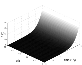
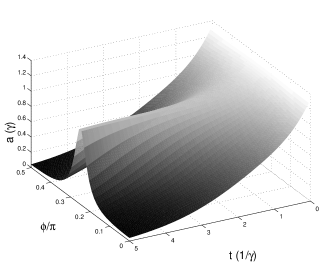
IV Conclusion

In summary, we have derived and studied the master equations for impurity bound electrons (qubits) scattering a bath of conduction electrons in a semiconductor. We show that the distribution of bath electrons remains Boltzmann at all temperatures, due to the temperature dependent filling of the conduction band. Thus our analysis, based on this result, is in contrast with other studies on decoherence of qubits in an electron gas obeying a Fermi-Dirac distribution Rikitake et al. (2004); Kim et al. (2004). The master equations are obtained in the Lindblad form for a single qubit and a system of two mutually non-interacting qubits. In the former, the Lindblad operators are found to be the spin operators for the qubit. In the latter, these are replaced by the sum and difference of the spin operators of each member of the system. The Bloch equations derived for a single qubit show that decoherence occurs at the same rate as relaxation in the $S^{z}$ basis. This departs from the conventional inequality $2T_{2}\leq T_{1}$ because the two levels in the system are degenerate, and therefore relaxation and dephasing processes are both elastic. The inverse relaxation times are equal to $\gamma$, which is proportional to the product of thermal flux of the bath electrons and an effective cross section that depends on the exchange coefficient $J$ and the Bohr radius of the qubit. Calculations show that $\gamma^{-1}$ is on the order of seconds for temperatures below 10 K, and decreases rapidly to below a microsecond above 70 K. Thus the conduction electron bath is dominant in causing decoherence compared to other sources Kane (1998); deSousa and DasSarma (2003); Hu and DasSarma (2003); Loss and DiVincenzo (1998); Koiller et al. (2002) for temperatures above 70K.

The same parameter $\gamma$ also sets the timescale of decoherence and relaxation in a two qubit system. However an additional parameter, $\xi(R_{T})$, representing the indirect exchange coupling of the two members of the system, affects the rates profoundly. The function $\xi(R_{T})$ decreases monotonically from one to zero with $R_{T}$, the ratio of inter-qubit distance to thermal deBroglie wavelength of conduction electrons. The dissipative part of the dynamical map is dominated by the total spin operator when $\xi\approx 1$. As a result the singlet state, with zero total spin, becomes the most robust state in this limit. For small $\xi$, however, the separable states in which both members of the system are in an eigenstate of the same Cartesian component of the spin operator exhibit the slowest rate of loss in purity. Pairs of Bell states are found to dephase independently of each other, and their dephasing rate never exceeds the population transfer rate. The unitary RKKY interaction arises naturally between the two qubits in our master equation. The frequency shift associated with this interaction is found to be proportional to the free electron susceptibility of the bath, in agreement with past studies of RKKY interaction between two spins mediated by a gas of free electrons Kim et al. (1995); Larsen (1981). While these studies found the interaction to decay exponentially as a function of inter-qubit distance for a Fermi-Dirac distribution, we find a Gaussian decay for a Boltzmann distributed electron gas. The results in the two qubit system can be understood qualitatively in terms of the coherence length of the bath electrons and the initial entanglement between the qubits. Electrons with large thermal deBroglie wavelength tend to scatter as if the two qubits were acting as a single entity, while those with small wavelength scatter off each qubit independently of the other. Similarly, qubits prepared in pure separable states lose purity independently of $\xi$, while the sensitivity to $\xi$ is much greater for entangled initial states.

The generalization to include the effects of an external magnetic field is straightforward and will restore the inequality $2T_{2}\leq T_{1}$ in addition to the precession of qubits in the field. However, interactions among the qubits demand a more involved calculation, because unless they are much larger or much smaller than the system-bath interaction, they render the secular approximation invalid. This approximation is central to most derivations of a coarse-grained, Markovian master equation.

Appendix A Derivation of master equation

Here we derive the master equation (7) of section 2. The density operator, denoted $W(t)$, for the joint qubit-electron system evolves unitarily via the transformation $W(t)=U(t)W(0)U^{\dagger}(t)$, where the unitary operator $U=1+iT$ and $T$ satisfies the equation

$$T = -\frac{1}{\hbar}\int_{0}^{t}H_{I}(t^{\prime})dt^{\prime}-\frac{i}{\hbar}\int_{0}^{t}H_{I}(t^{\prime})T(t^{\prime})dt^{\prime}.$$ (42)

By unitarity of $U(t)$ it follows that $i(T-T^{\dagger})=-T^{\dagger}T$, and the evolution of $W(t)$ can then be written in terms of $T$ as

$$W(t)-W(0) = \frac{i}{2}[T+T^{\dagger},W(0)]+TW(0)T^{\dagger}-\frac{1}{2}T^{\dagger}TW(0)-\frac{1}{2}W(0)T^{\dagger}T.$$ (43)

We consider only the product initial state, $W(0)=\rho_{0}\otimes R_{B}$, where $R_{B}$ is the thermal density matrix of the bath. We first show that under the second order Born approximation and appropriate coarse-graining of $t$, (43) yields the following equation for the system density matrix:

$$\rho(t)-\rho_{0} = -i\sum_{ijkl}tN_{ijkl}[\eta_{ij}\eta_{kl},\rho_{0}]+\sum_{ijkl}tM_{ijkl}(2\eta_{ij}\rho_{0}\eta_{kl}-\eta_{kl}\eta_{ij}\rho_{0}-\rho_{0}\eta_{kl}\eta_{ij}).$$ (44)

The tensors $N_{ijkl}$ and $M_{ijkl}$ are independent of time, and $\eta_{ij}$ are system operators defined by $\eta_{ij}=\left|i\right\rangle\left\langle j\right|$.

We derive each sum in (44) from the corresponding term in (43), correct to second order. Since the expansion of $T$ starts at the first order in $H_{I}$, the dissipative term becomes second order automatically. Application of the first order expansion of $T$ then yields the second sum in (44) with the tensor $M_{ijkl}$ given by the expression:

$$tM_{ijkl} = \frac{1}{2\hbar^{2}}\int_{0}^{t}dt^{\prime}\int_{0}^{t}dt^{\prime\prime}\sum_{\alpha,\alpha^{\prime}}\sum_{\mathbf{p},\mathbf{p}^{\prime}}e^{i(\omega_{p}-\omega_{p^{\prime}})(t^{\prime\prime}-t^{\prime})}\left\langle\alpha\mathbf{p};i\right|V\left|\alpha^{\prime}\mathbf{p}^{\prime};j\right\rangle\left\langle\alpha^{\prime}\mathbf{p}^{\prime};k\right|V\left|\alpha\mathbf{p};l\right\rangle\mathcal{N}_{\mathbf{p}},$$ (45)

where $\mathcal{N}_{\mathbf{p}}$ is the number of particles in the momentum state $\mathbf{p}$. We now evaluate the integrals and sums in the limit of a large crystal. Let $\Omega$ represent the crystal volume, and within this volume, let $n(\mathbf{p})$ be the density of conduction electrons in the phase space. Then $\mathcal{N}_{\mathbf{p}}=\Omega\Delta\mathbf{p}n(\mathbf{p})$, where $\Delta\mathbf{p}=(2\pi\hbar)^{3}/\Omega$ is the volume in $\mathbf{p}$-space associated with a momentum state. Introducing the phase space volume for $\mathbf{p}^{\prime}$ in a similar manner and letting $\Omega$ be large we find that

$$\sum_{\mathbf{p}}\mathcal{N}_{\mathbf{p}}\sum_{\mathbf{p}^{\prime}} \rightarrow \int d\mathbf{p}\Omega n(\mathbf{p})\int d\mathbf{p}^{\prime}\frac{\Omega}{(2\pi\hbar)^{3}}.$$

Next we introduce the rescaled operators $\tilde{V}_{ij}=\Omega(2\pi\hbar)^{-3}\left\langle i\right|V\left|j\right\rangle$ and substitute them in (45). Making a change of variables in $t^{\prime},t^{\prime\prime}$ we find that

$$tM_{ijkl} = 4\pi^{3}\hbar\sum_{\alpha\alpha^{\prime}}\int_{0}^{t}d\tau^{\prime}\int_{-L(t;\tau^{\prime})}^{+L(t;\tau^{\prime})}d\tau\int d\mathbf{p}d\mathbf{p}^{\prime}e^{i(\omega_{p}-\omega_{p^{\prime}})\tau}n(\mathbf{p})\left\langle\alpha\mathbf{p}\right|\tilde{V}_{ij}\left|\alpha^{\prime}\mathbf{p}^{\prime}\right\rangle\left\langle\alpha^{\prime}\mathbf{p}^{\prime}\right|\tilde{V}_{kl}\left|\alpha\mathbf{p}\right\rangle,$$

where $L(t;\tau^{\prime})=2\tau^{\prime}$ for $\tau^{\prime}\leq t/2$ and $L(t;\tau^{\prime})=2(\tau-\tau^{\prime})$ for $\tau\leq t/2$. The integral over $\tau$ is essentially a Fourier transform of a $p-$dependent function and it is expected to drop quickly for thermal distributions at sufficiently high temperatures Carmichael (1999). Therefore, we switch to a coarse-grained timescale which captures the evolution of the qubit but not the behavior of the bath correlations. In this limit, $L(t;\tau^{\prime})$ may be considered infinite for essentially all $\tau^{\prime}$ without introducing error in the integral over $\tau$. The result is

$$tM_{ijkl} = t8\pi^{4}\hbar\sum_{\alpha\alpha^{\prime}}\int d\mathbf{p}d\mathbf{p}^{\prime}n(\mathbf{p})\delta(\frac{p^{\prime 2}-p^{2}}{2m\hbar})\left\langle\alpha\mathbf{p}\right|\tilde{V}_{ij}\left|\alpha^{\prime}\mathbf{p}^{\prime}\right\rangle\left\langle\alpha^{\prime}\mathbf{p}^{\prime}\right|\tilde{V}_{kl}\left|\alpha\mathbf{p}\right\rangle.$$ (46)

The factor $t$ appears from the integral over $\tau^{\prime}$ due to the absence of system dynamics; in the presence of system dynamics, $\tau^{\prime}$ is coarse-grained further to be insensitive to the energy difference between the system levels. We now integrate over $\mathbf{p}^{\prime}$ making use of the formula $n(\mathbf{p})d\mathbf{p}=4\pi p^{2}n(p)dp(d\mathbf{\hat{\mathbf{u}}}/4\pi)$, where $n(p)$ is the occupancy of energy state $p^{2}/2m$ divided by phase space cell volume, and $d\hat{\mathbf{u}}$ is an element of the solid angle centered about $\hat{\mathbf{u}}$. After substituting these definitions we find that

$$M_{ijkl} = 2(2\pi)^{6}(m\hbar)^{2}\int_{0}^{\infty}dp\frac{p}{m}p^{2}n(p)\sum_{\alpha\alpha^{\prime}}\int\frac{d\mathbf{\hat{\mathbf{u}}}}{4\pi}\frac{d\mathbf{\hat{\mathbf{u}}}^{\prime}}{4\pi}\left\langle\alpha p\mathbf{\hat{\mathbf{u}}}\right|\tilde{V}_{ij}\left|\alpha^{\prime}p\mathbf{\hat{\mathbf{u}}}^{\prime}\right\rangle\left\langle\alpha^{\prime}p\mathbf{\hat{\mathbf{u}}}^{\prime}\right|\tilde{V}_{kl}\left|\alpha p\mathbf{\hat{\mathbf{u}}}\right\rangle.$$ (47)

In a similar treatment Hornberger and Sipe (2003) it was shown that a more accurate calculation yields a result obtained by replacing the first order scattering amplitudes in this formula with their exact counterparts. We expect the same to hold here, but since the exchange interaction is often introduced with parameters assumed appropriate for only a lowest order Born calculation, we do not pursue this issue here. We finalize this formula by substituting the Boltzmann distribution for $n(p)$,

$$n(p) = n_{c}(2\pi mk_{B}T)^{-\frac{3}{2}}e^{-p^{2}/2mk_{B}T},$$

where we remind the reader that $n_{c}$ is the total number of conduction electrons present at temperature $T$. It is convenient to introduce the dimensionless variable $x=(2mk_{B}T)^{-1}p^{2}$ in terms of which ($v=4(2\pi)^{9/2}n_{c}(m\hbar)^{2}\sqrt{k_{B}T/m}$)

$$M_{ijkl} = v\int_{0}^{\infty}dxxe^{-x}\int\frac{d\mathbf{\hat{\mathbf{u}}}}{4\pi}\frac{d\mathbf{\hat{\mathbf{u}}}^{\prime}}{4\pi}\sum_{\alpha\alpha^{\prime}}\left\langle\alpha,p\mathbf{\hat{\mathbf{u}}}\right|\tilde{V}_{ij}\left|\alpha^{\prime},p\mathbf{\hat{\mathbf{u}}}^{\prime}\right\rangle\left\langle\alpha^{\prime},p\mathbf{\hat{\mathbf{u}}}^{\prime}\right|\tilde{V}_{kl}\left|\alpha,p\mathbf{\hat{\mathbf{u}}}\right\rangle.$$ (48)

Our next task is to expand $i\mathsf{Tr}_{B}(T+T^{\dagger})/2$ and obtain a time-independent expression for $N_{ijkl}$. As the bath distribution does not depend on spin, the first order term vanishes by the zero trace property of Pauli matrices. The second order term then yields,

$$\frac{i}{2}\mathsf{Tr}_{B}[T+T^{\dagger},W_{0}] = \frac{-1}{2\hbar^{2}}\int_{0}^{t}dt^{\prime}\int_{0}^{t^{\prime}}d\tau\mathsf{Tr}_{B}[[H_{I}(t^{\prime}),H_{I}(t^{\prime}-\tau)],\rho_{0}\otimes R_{B}].$$ (49)

The commutator $[H_{I}(t^{\prime}),H_{I}(t^{\prime}-\tau)]$ takes the following form where the summation is done over all $\mathbf{p}$ and $\alpha$:

$$[H_{I}(t^{\prime}),H_{I}(t^{\prime}-\tau)] = \eta_{ij}\eta_{kl}\sum e^{i(\omega_{p^{\prime\prime}}-\omega_{p})t^{\prime}}\left(e^{i(\omega_{p^{\prime}}-\omega_{p})\tau}-e^{-i(\omega_{p^{\prime}}-\omega_{p^{\prime\prime}})\tau}\right)$$

$$\times\left|\alpha\mathbf{p}\right\rangle\left\langle\alpha\mathbf{p}\right|V_{ij}\left|\alpha^{\prime}\mathbf{p}^{\prime}\right\rangle\left\langle\alpha^{\prime}\mathbf{p}^{\prime}\right|V_{kl}\left|\alpha^{\prime\prime}\mathbf{p}^{\prime\prime}\right\rangle\left\langle\alpha^{\prime\prime}\mathbf{p}^{\prime\prime}\right|.$$

We convert the summations over momentum to integrals and substitute the result in (49). Taking the trace we find

$$\frac{i}{2}\mathsf{Tr}_{B}[T+T^{\dagger},W_{0}] = [\eta_{ij}\eta_{kl},\rho_{0}]t(-4\pi^{3}\hbar)\sum_{\alpha,\alpha^{\prime}}\int d\mathbf{p}d\mathbf{p}^{\prime}$$ (50)

$$\int_{0}^{\infty}d\tau 2i\sin[(\omega_{p^{\prime}}-\omega_{p})\tau]\left\langle\alpha\mathbf{p}\right|\tilde{V}_{ij}\left|\alpha^{\prime}\mathbf{p}^{\prime}\right\rangle\left\langle\alpha^{\prime}\mathbf{p}^{\prime}\right|\tilde{V}_{kl}\left|\alpha\mathbf{p}\right\rangle n(\mathbf{p}).$$

The integral over $\tau$ yields $2i\mathcal{P}(\omega_{p}-\omega_{p^{\prime}})^{-1}$, where $\mathcal{P}$ denotes the principal value. Comparing (50) with (44), we get

$$N_{ijkl} = 4\pi^{3}\hbar\int d\mathbf{p}d\mathbf{p}^{\prime}\frac{2\mathcal{P}}{\omega_{p^{\prime}}-\omega_{p}}n(\mathbf{p})\sum_{\alpha,\alpha^{\prime}}\left\langle\alpha\mathbf{p}\right|\tilde{V}_{ij}\left|\alpha^{\prime}\mathbf{p}^{\prime}\right\rangle\left\langle\alpha^{\prime}\mathbf{p}^{\prime}\right|\tilde{V}_{kl}\left|\alpha\mathbf{p}\right\rangle].$$ (51)

Substitution of the Boltzmann distribution and re-expression in terms of the dimensionless variable defined above yields the following expression:

$$N_{ijkl} = \frac{v}{\pi}\int dxdy\sqrt{xy}e^{-x}\frac{\mathcal{P}}{y-x}\int\frac{d\mathbf{\hat{\mathbf{u}}}}{4\pi}\frac{d\mathbf{\hat{\mathbf{u}}}^{\prime}}{4\pi}\sum_{\alpha,\alpha^{\prime}}\left\langle\alpha\mathbf{p}\right|\tilde{V}_{ij}\left|\alpha^{\prime}\mathbf{p}^{\prime}\right\rangle\left\langle\alpha^{\prime}\mathbf{p}^{\prime}\right|\tilde{V}_{kl}\left|\alpha\mathbf{p}\right\rangle.$$ (52)

Having shown the validity of (44), we can obtain a coarse-grained differential equation for $\rho(t)$ by iterating this equation after replacing $\rho(t)-\rho(0)$ by $\rho(t+\delta t)-\rho(t)$. Thus

$$\frac{d\rho}{dt} = -i\sum_{ijkl}N_{ijkl}[\eta_{ij}\eta_{kl},\rho]+\sum_{ijkl}M_{ijkl}(2\eta_{kl}\rho\eta_{ij}-\eta_{ij}\eta_{kl}\rho-\rho\eta_{ij}\eta_{kl}).$$ (53)

When the expressions (4) and (5) are substituted for $V$, the tensor $M$ becomes $\gamma\Lambda$, where $\gamma$ is a constant defined in (8) and $\Lambda$ is given by (11) for the single qubit and by (17) for the two qubit system. The commutator associated with the tensor $N$ vanishes for the single qubit. In the two qubit system, the tensor $N=\omega_{RKKY}\Gamma$, where $\omega_{RKKY}$ is defined in (9), while $\Gamma$ is given by (18).

We now outline the calculation to obtain the RKKY splitting in terms of the susceptibility of the bath. We first observe that (51) can be written as

$$N_{ijkl} = 4\pi^{3}\hbar\int d\mathbf{p}d\mathbf{p}^{\prime}2\Re\left(\frac{1}{\omega_{p^{\prime}}-\omega_{p}+i\epsilon}\right)n(\mathbf{p})\sum_{\alpha,\alpha^{\prime}}\left\langle\alpha\mathbf{p}\right|\tilde{V}_{ij}\left|\alpha^{\prime}\mathbf{p}^{\prime}\right\rangle\left\langle\alpha^{\prime}\mathbf{p}^{\prime}\right|\tilde{V}_{kl}\left|\alpha\mathbf{p}\right\rangle],$$

where $\epsilon\rightarrow 0$ at the end of the calculation. Substituting (5) in the above expression, keeping only the cross-terms, and changing the variables of integration to $\mathbf{k}=\mathbf{p}/\hbar$, we find that

$$N_{ijkl} = \Gamma_{ijkl}4\pi^{3}\hbar^{-2}(Jr_{0}^{3})^{2}\int\frac{d\mathbf{k}}{(2\pi)^{3}}\frac{d\mathbf{k}^{\prime}}{(2\pi)^{3}}n(\mathbf{k})e^{i(\mathbf{k}^{\prime}-\mathbf{k})\cdot\mathbf{R}}2\Re\left(\frac{1}{\omega_{k^{\prime}}-\omega_{k}+i\epsilon}\right)+c.c.$$

Here $\mathbf{k},\mathbf{q}$ are wave-vectors, $n(\mathbf{k})d\mathbf{k}$ now represents the density of electrons with wave-vector within $d\mathbf{k}$ of $\mathbf{k}$, and $\Gamma_{ijkl}$ represents the summation over spin indices $\alpha,\alpha^{\prime}$. We now manipulate the sum by first writing it as a sum of two identical copies of itself and then interchanging $\mathbf{k},\mathbf{k}^{\prime}$ in one of the integrals. Then doing the transformation $\mathbf{k},\mathbf{k}^{\prime}\rightarrow-\mathbf{k},-\mathbf{k}^{\prime}$ in that integral, we find that

$$N_{ijkl} = \Gamma_{ijkl}4\pi^{3}\hbar^{-2}(Jr_{0}^{3})^{2}\left[\int\frac{d\mathbf{k}}{(2\pi)^{3}}\frac{d\mathbf{k}^{\prime}}{(2\pi)^{3}}e^{i(\mathbf{k}^{\prime}-\mathbf{k})\cdot\mathbf{R}}n(\mathbf{k})\Re\left(\frac{1}{\omega_{k^{\prime}}-\omega_{k}+i\epsilon}\right)\right.$$

$$\left.-\int\frac{d\mathbf{k}}{(2\pi)^{3}}\frac{d\mathbf{k}^{\prime}}{(2\pi)^{3}}e^{i(\mathbf{k}^{\prime}-\mathbf{k})\cdot\mathbf{R}}n(\mathbf{k})\Re\left(\frac{1}{\omega_{k^{\prime}}-\omega_{k}+i\epsilon}\right)+c.c\right].$$

We do not change the sign of $i\epsilon$ in the second integral since the real part is unaffected by it. An expression equivalent to the one above is

$$N_{ijkl} = -\Gamma_{ijkl}4\pi^{3}\hbar^{-1}(Jr_{0}^{3})^{2}\int\frac{d\mathbf{q}}{(2\pi)^{3}}e^{i\mathbf{q}\cdot\mathbf{R}}\int\frac{d\mathbf{k}}{(2\pi)^{3}}\frac{[n(\mathbf{k}+\frac{1}{2}\mathbf{q})-n(\mathbf{k}-\frac{1}{2}\mathbf{q})]}{\hbar^{2}\mathbf{k}\cdot\mathbf{q}/m+i\epsilon}+c.c.$$

The integral over $\mathbf{k}$ in the limit $\epsilon=0$ is the static Lindhard function Ashcroft and Mermin (1976), which defines the Fourier transform, $\chi(\mathbf{q})$, of the static susceptibility $\chi(\mathbf{r})$ Kim et al. (1995, 1999). Since $\chi(\mathbf{r})=\chi(-\mathbf{r})$,

$$N_{ijkl} = -(2\pi)^{3}\hbar^{-1}(Jr_{0}^{3})^{2}\chi(\mathbf{R})\Gamma_{ijkl}.$$

References

- Abrahams (1957) E. Abrahams, Phys. Rev. 107, 491 (1957).
- Pines et al. (1957) D. Pines, J. Bardeen, and C. Slitcher, Phys. Rev. 106, 489 (1957).
- Honig (1954) A. Honig, Phys. Rev. 96, 294 (1954).
- Kane (1998) B. E. Kane, Nature 393, 134 (1998).
- Hu and DasSarma (2003) X. Hu and S. DasSarma, Phys. Stat. Sol. (b) 238, 360 (2003).
- Koiller et al. (2002) B. Koiller, X. Hu, and S. DasSarma, PRL 88, 027903 (2002).
- Loss and DiVincenzo (1998) D. Loss and D. P. DiVincenzo, Phys. Rev. A. 57, 120 (1998).
- deSousa and DasSarma (2003) R. deSousa and S. DasSarma, Phys. Rev. B 68, 115322 (2003).
- Kim et al. (2004) W. Kim, R. K. Teshima, and F. Marsiglio (2004), eprint cond-mat/0410775.
- Rikitake et al. (2004) Y. Rikitake, H. Imamura, and H. Ebisawa (2004), eprint cond-mat/0408375.
- Kohn and Luttinger (1955) W. Kohn and J. Luttinger, Phys. Rev. 98, 915 (1955).
- Feher et al. (1955) Feher, Fletcher, and Gere, Phys. Rev. 100, 1784 (1955).
- Tyryshkin et al. (2003) A. M. Tyryshkin, S. A. Lyon, A. V. Astashkin, and A. M. Raitsimring, Phys. Rev. B 68, 193207 (2003).
- L.D. Chang (1984) S. C. L.D. Chang, Phys. Rev. B 31, 154 (1984).
- Chen (1987a) Y. Chen, J. Stat. Phys. 47, 17 (1987a).
- Chen (1987b) Y. Chen, J. Stat. Phys. 49, 811 (1987b).
- Chen (1987c) Y. Chen, Phys. Rev. A 37, 3450 (1987c).
- Larsen (1981) U. Larsen, Physics Letters 85A, 471 (1981).
- Kim et al. (1995) J. G. Kim, E. K. Lee, and S. Lee, Phys. Rev. B 51, R670 (1995).
- Bloch (1946) F. Bloch, Phys. Rev. 70, 460 (1946).
- Carmichael (1999) H. Carmichael, Statistical methods in quantum optics 1: master equations and Fokker-Planck equations (Springer, Berlin, 1999).
- Hornberger and Sipe (2003) K. Hornberger and J. E. Sipe, Phys. Rev. A 68, 012105 (2003).
- Ashcroft and Mermin (1976) Ashcroft and Mermin, Solid State Physics (Brooks/Cole, 1976).
- Kim et al. (1999) J. G. Kim, Y.-H. Choi, E. K. Lee, and S. Lee, Phys. Rev. B 59, 3661 (1999).