Reconstruction of the phase of matter-wave fields using a momentum resolved cross-correlation technique

Abstract

We investigate the potential of the so-called XFROG cross-correlation technique originally developed for ultrashort laser pulses for the recovery of the amplitude and phase of the condensate wave function of a Bose-Einstein condensate. Key features of the XFROG method are its high resolution, versatility and stability against noise and some sources of systematic errors. After showing how an analogue of XFROG can be realized for Bose-Einstein condensates, we illustrate its effectiveness in determining the amplitude and phase of the wave function of a vortex state. The impact of a reduction of the number of measurements and of typical sources of noise on the field reconstruction are also analyzed.

Many of the remarkable properties of atomic Bose-Einstein condensates (BECs) originate from the fact that in those systems a single wave-function is occupied by a macroscopic number of particles Davis et al. (1995); Bradley et al. (1995); Anderson et al. (1995); Ketterle and H.-J. Miesner (1997); Andrews et al. (1997). The amplitude of this complex wave function corresponds to the atomic density and can comparatively easily be measured using for example absorption or phase contrast imaging You et al. (1996); You and Lewenstein (1996); Politzer (1995, 1997); Ketterle et al. (1999). The phase of the wave function, on the other hand, is relatively hard to measure directly. Still, its measurement is essential for the characterization of many quantum-degenerate atomic systems, such as e.g. rotating BECs with vortices Matthews et al. (1999).

A situation in many ways similar is encountered in the context of ultrashort laser pulses of a few optical cycles duration. The characterization of these pulses, which are of considerable interest in both fundamental science and applications, requires likewise the knowledge of both amplitude and phase.

The measurement of the time-dependent phase of ultrashort laser pulses has found a solution that is in many respects optimal in the so-called Frequency-Resolved Optical Gating (FROG) methods J. L. A. Chilla and O. E. Martinez (1991); Kane and Trebino (1993a); DeLong et al. (1994); Trebino and Kane (1993). These methods, which can be adapted to many different situations, offer very high resolution and precision, are stable against noise, and can even compensate for or detect some sources of systematic errors. Single-shot measurements are straightforward Kane and Trebino (1993b), and measurements of fields with less than one photon per pulse on average have also been successfully demonstrated. Almost every aspect of the FROG-methods has been studied in depth. Good starting points for accessing the wealth of research literature on that subject are the review article Trebino et al. (1997) and Ref. Trebino (2000).

The similarity of the phase-retrieval problems for ultrashort pulses and atomic condensates naturally leads one to ask whether the optical FROG techniques can be extended to the atom-optical domain. This paper answers this question in the affirmative by demonstrating how a specific version of the general FROG method, called cross-correlation FROG (XFROG), can easily be translated to the atom-optical case Linden et al. (1999, 1998, 2000).

Section I briefly reviews the fundamentals of XFROG phase retrieval and discusses how it can be adapted to cold-atom scenarios. As an illustration, section II shows the reconstruction of the spatial phase of a rotating BEC with a vortex. We also investigate the sensitivity of the reconstruction to several sources of noise characteristic of cold atoms, as well as the impact of a reduction in the number of measurements on the field retrieval.

I Principles of the XFROG method

The basic experimental setup for the field reconstruction of an ultrashort laser pulse by means of the XFROG method is shown in Fig. 1. For simplicity we assume that only one direction of polarization of the electrical field needs to be considered. The unknown field $\psi(t)$ is mixed with a known reference field $\psi_{\rm ref}(t)$ in a nonlinear crystal with $\chi^{(2)}$ nonlinearity after a variable delay $\tau$. The fields $\psi_{\rm ref}$ and $\psi$ should be of roughly comparable duration which means in practice that the pulse durations can differ by up to about an order of magnitude. The sum frequency signal is

$$\psi_{\rm sig}(t,\tau)\propto\psi(t)\psi_{\rm ref}(t-\tau).$$ (1)

The form of that field shows that the reference pulse acts as a gate for the pulse, hence the acronym XFROG. The signal $\psi_{\rm sig}$ is then spectrally analyzed. The resulting spectrum,

$$I_{\rm XFROG}(\omega,\tau) \equiv \left|\int dte^{-i\omega t}\psi_{\rm sig}(t,\tau)\right|^{2}$$ (2)

$$= \left|\int dte^{-i\omega t}\psi(t)\psi_{\rm ref}(t-\tau)\right|^{2},$$

is the key quantity. It contains enough information to reconstruct amplitude and phase of the pulse $\psi(t)$.

Figure 1: (Color online) Basic experimental setup for the XFROG method. G is a diffraction grating and the spectrum of the signal field is recorded with the CCD array.

To see how this works , we first note that it is sufficient to find $\psi_{\rm sig}(t,\tau)$ since $\psi(t)$ can then be obtained by simply integrating over $\tau$ — up to a multiplicative constant that can be determined from the normalization of $\psi$. Thus the problem is cast in the form of a two-dimensional phase retrieval problem. Problems of this type have been studied for decades in the context of image restoration, see e.g. Fienup (1982); Yudilevich et al. (1987).

The field $\psi_{\rm sig}$ can be found from $I_{\rm XFROG}$ by means of the method of generalized projections DeLong and Trebino (1994); Yudilevich et al. (1987); Kenneth W. DeLong et al. (1994). From Eqs. (1) and (2) it is clear that $\psi_{\rm sig}$ must simultaneously belong to the two sets

$$O=\left\{f(t,\tau)|f(t,\tau)=g(t)\psi_{\rm ref}(t-\tau)\text{ for some }g\right\}$$ (3)

and

$$F=\left\{f(t,\tau)|\left|\int dte^{-i\omega t}f(t,\tau)\right|^{2}=I_{\rm XFROG}(\omega,\tau)\right\}.$$ (4)

Hence, the solution is a field that satisfies the two constraints

$$\psi_{\rm sig}(t,\tau)\in O\cap F.$$ (5)

Figure 2a suggests that one can find the solution to this problem, called a feasibility problem in mathematics and especially in optimization theory, by iteratively projecting onto the two constraint sets $O$ and $F$. For closed convex sets with exactly one point of intersection, this method always leads to a unique solution. In our case, though, the constraint sets are not convex and their intersection consists of more than one function, as illustrated in Fig. 2b. Hence, the algorithm of generalized projections is not guaranteed to converge for every initial guess and even if it does the solution is not unique. Still, in practice it converges for a vast majority of initial guesses and the ambiguity in the solution is physically reasonable. (In particular, XFROG determines the field $\psi_{\rm sig}$ up to a constant phase.) On those rare occasions when the algorithm does not converge for a particular initial guess, this non-convergence is revealed by a large distance of the fixed point from the constraint sets in a sense that will be made precise below. Then one can simply restart the reconstruction algorithm with a different initial guess.

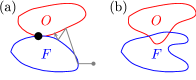
Figure 2: (Color online) Illustration of the constraint sets $O$ and $F$ (a) in the case where $O$ and $F$ are convex and their intersection contains exactly one element and (b) in the non-convex case with more than one element in the intersection. Fig. (a) also shows a typical trajectory of the generalized projections algorithm.

Specifically, $\psi_{\rm sig}$ is found from $I_{\rm XFROG}$ as follows:

1. Initialize $\tilde{\psi}_{\rm sig}^{(0)}(\omega,\tau)$ with random numbers for its real and imaginary part.

2. The projection onto the constraint set $F$ is accomplished by setting

   $$\psi_{\rm sig}^{(n)}(\omega,\tau)=\frac{\tilde{\psi}_{\rm sig}^{(n-1)}(\omega,\tau)}{|\tilde{\psi}_{\rm sig}^{(n-1)}(\omega,\tau)|}I_{\rm FROG}^{1/2}(\omega,\tau),$$ (6)

   which clearly guarantees that $\psi_{\rm sig}^{(n)}$ satisfies condition (4).

3. Inverse Fourier transform $\psi_{\rm sig}^{(n)}(\omega,\tau)$ with respect to the first argument to find

   $$\psi_{\rm sig}^{(n)}(t,\tau)=\int\frac{d\omega}{2\pi}e^{i\omega t}\psi_{\rm sig}^{(n)}(\omega,\tau).$$ (7)

4. Determine $\psi^{(n)}(t)$ such that

   $$Z=\int dtd\tau\left|\psi_{\rm sig}^{(n)}(t,\tau)-\psi^{(n)}(t)\psi_{\rm ref}(t-\tau)\right|^{2}$$ (8)

   becomes a minimum. With $\psi^{(n)}(t)$ determined this way form

   $$\tilde{\psi}_{\rm sig}^{(n)}(t,\tau)=\psi^{(n)}(t)\psi_{\rm ref}(t-\tau),$$ (9)

   which is closer to the set $O$ than $\psi_{\rm sig}^{(n)}(t,\tau)$.

5. Use the Fourier transform

   $$\tilde{\psi}_{\rm sig}^{(n)}(\omega,\tau)=\int dte^{-i\omega t}\tilde{\psi}_{\rm sig}^{(n)}(t,\tau)$$ (10)

   as a new input in step 2, and iterate until the error $Z$ in Eq. (8) becomes sufficiently small.

Upon exit from the algorithm, $\psi^{(n)}$ is the retrieved field. It turns out that in step 4 a simple line minimization along the gradient of $Z$ with respect to $\psi^{(n)}$ is sufficient. A good starting point for that minimization is the minimizer $\psi^{(n-1)}$ of the previous step.

An important characteristic of the XFROG method is its robustness, which results from two main reasons: First, the XFROG signal contains a high degree of redundancy: If $I_{\rm XFROG}$ is measured on a grid of size $N\times N$ the $2N$ unknowns of the field $\psi(t)$ – its real and imaginary parts – are retrieved from $N^{2}$ measured values. The XFROG algorithm makes use of this high degree of redundancy to yield a highly stable pulse retrieval. Second, the functional form of $\psi_{\rm sig}$ is very restrictive in the sense that a randomly generated $\psi_{\rm sig}$ will not correspond to any physical pulse $\psi$. Thus, if the XFROG signal has been deteriorated by systematic errors the XFROG algorithm will not converge for any initial guess and one can conclude that the data is corrupted. Another advantage of XFROG is the extremely high temporal resolution that is achieved by making use of the Fourier domain information. Instead of being determined by the length of the reference pulse, it is essentially given by the response time of the non-linear medium.

We now turn to the central point of this paper, which is to adapt the XFROG method to the characterization of matter-wave fields. We consider specifically the case of atomic bosons, with two internal states denoted by $\uparrow$ and $\downarrow$. The atoms are assumed to be initially in a pure Bose-Einstein condensate (BEC) at temperature $T=0$, with all atoms in internal state $\downarrow$. The corresponding atomic field operator is

$$\hat{\psi}({\bf{r}})=\hat{c}_{\downarrow}\psi({\bf{r}}),$$ (11)

where $\psi({\bf{r}})$ is the condensate wave function and $\hat{c}_{\downarrow}$ is the bosonic annihilation operator for an atom in the condensate.

The states $\uparrow$ and $\downarrow$ are coupled by a spatially dependent interaction of the generic form

$$V_{J}=\int d^{3}r{V}({\bf{r}}-{\bf{R}})\hat{\psi}_{\uparrow}^{\dagger}({\bf{r}})\hat{\psi}_{\downarrow}({\bf{r}})+H.c.$$ (12)

that is switched on at time $t=0$. This could be provided for example by a two-photon Raman transition, with $V$ then being proportional to the product of the mode functions of the two lasers driving the transition.

For short enough times the $\uparrow$-component of the atomic field is then

$$\hat{\psi}_{\uparrow}({\bf{r}})\propto\tilde{V}({\bf{r}}-{\bf{R}})\hat{\psi}_{\downarrow}({\bf{r}}).$$ (13)

The resulting momentum distribution of the $\uparrow$-atoms is

$$n({\bf{q}},{\bf{R}}) \propto \int d^{3}rd^{3}r^{\prime}e^{i{\bf{q}}{\bf{r}}}e^{-i{\bf{q}}{\bf{r}}^{\prime}}\left\langle\hat{\psi}_{\uparrow}^{\dagger}({\bf{r}})\hat{\psi}_{\uparrow}({\bf{r}}^{\prime})\right\rangle$$ (15)

$$\propto \int d^{3}rd^{3}r^{\prime}e^{i{\bf{q}}{\bf{r}}}e^{-i{\bf{q}}{\bf{r}}^{\prime}}$$

$$\times\psi^{*}({\bf{r}})V^{*}({\bf{r}}-{\bf{R}})\psi({\bf{r}}^{\prime})V({\bf{r}}^{\prime}-{\bf{R}})$$

$$= \left|\int d^{3}re^{-i{\bf{q}}{\bf{r}}}\psi({\bf{r}})V({\bf{r}}-{\bf{R}})\right|^{2}.$$ (16)

When measured as a function of the shift ${\bf{R}}$ between coupling and condensate, the momentum distribution of the $\uparrow$-atoms is therefore an XFROG signal, with the role of the reference field being played by the space dependent coupling strength. Hence, the XFROG algorithm can be used to fully recover the field $\psi$, $n({\bf q},{\bf R})$ being measured using for example absorption imaging after free expansion.

In some sense, the situation for atoms is simpler than for ultrashort laser pulses. This is because a gate function of size comparable to the condensate size, such as e.g. the coupling strength $V({\bf{r}})$, is readily available. While in the case of photons the only possible gate is another ultrashort laser pulse, and hence one must use nonlinear mixing to obtain a signal suitable for XFROG, for atoms one can use processes that are linear in the atomic field. Furthermore, since the interactions between cold atoms tend to be stronger and offer a richer variety than is the case for light, a wide choice of processes can be employed to generate signals that can be used for FROG algorithms. Specific examples include $s$-wave interactions, the atom-optics analog of optical cubic nonlinearities, as well as the recently demonstrated coherent coupling of atoms to molecules, which corresponds to optical quadratic nonlinearities Wynar et al. (2000); Inouye et al. (1998); Donley et al. (2002); Dürr et al. (2004); Greiner et al. (2003); Jochim et al. (2003).

A fully three-dimensional XFROG scheme as suggested by Eq. (16) is hard to realize in practice. First, it requires a very large number of measurements. Ten different shifts in each direction correspond to a total of 1000 runs of the experiment. The large amount of data necessary for the fully three-dimensional scheme also poses serious challenges to the numerical reconstruction algorithm as far as computer memory and time are concerned. Second, in time-of-flight absorption imaging one typically measures the column-integrated density so that the three-dimensional momentum distribution is not directly accessible. It appears therefore preferable to limit the reconstruction to have a two-dimensional scheme.

It can be easily verified that if the field $\psi$ and the coupling strength can be factorized as

$$\psi({\bf{r}})=f(z)\psi(x,y),\quad V({\bf{r}})=h(z)V(x,y),$$ (17)

where $z$ is the direction along which the imaging is done, Eq. (16) remains valid if we interpret ${\bf{r}}$ and ${\bf{R}}$ as two-dimensional vectors in the plane perpendicular to $z$ and ${\bf{q}}$ as a corresponding two-dimensional momentum. Many fields of practical interest can at least approximately be written in the form Eq. (17). For example, the two-photon Raman coupling mentioned earlier is of that type provided that the lasers are directed along $z$ and the Rayleigh length is much longer than the extend of the atomic cloud in that direction. As a concrete example we demonstrate in the next section how the matter wave field of a rotating BEC with a single vortex Matthews et al. (1999) can be directly reconstructed using the XFROG method.

II Reconstruction of a vortex-field

We consider a BEC at temperature $T=0$ in a spherical trap. We assume that the Thomas-Fermi approximation holds and that the healing length $\xi=(8\pi an_{0})^{-1/2}$, with $a$ the $s$-wave scattering length and $n_{0}$ the atomic density at the center of the trap, is much smaller than the Thomas-Fermi Radius $R=(15N_{a}a/a_{\rm osc})^{1/5}a_{\rm osc}$ of the cloud. Here, $N_{a}$ is the number of atoms in the condensate and $a_{\rm osc}$ is the oscillator length of the atoms in the trap. Under these assumptions the structure of the vortex core is essentially the same as that of a vortex in a uniform BEC and its wave function can to a good approximation be written as Pethick and Smith (2002)

$$\psi(r,\varphi,z)=f(z)\frac{r/R}{\sqrt{2(\xi/R)^{2}+(r/R)^{2}}}\sqrt{1-(r/R)^{2}}e^{i\varphi},$$ (18)

where we have used cylindrical coordinates with the vortex core at the symmetry axis. As discussed above, the $z$-dependence of the wave-function is unimportant and we will not regard it any further. In the following we use $\xi/R=0.1$, but none of our results depend strongly on this ratio as long as $\xi/R\ll 1$. The real part of the wave-function (18) is shown in Fig. 4a.

As an interaction Hamiltonian, or ‘reference field’ in the language of XFROG, we use Eq. (12) with the Gaussian

$$V(r)=e^{-(r/w)^{2}},$$ (19)

the $z$-dependence being again irrelevant for our purposes.

We have simulated an XFROG signal on a grid of $64\times 64$ points using $\psi$ of Eq. (18) and the reference field (19), and applied the XFROG algorithm to reconstruct the field. In order the determine the optimal width of $V$ we have repeated this procedure for various values of $w$. For each run we have determined the $\chi^{2}$-error per degree of freedom

$$\chi^{2}=\frac{1}{2N^{2}}\sum_{i,j}|\psi^{(n)}({\bf{r}}_{ij})-\psi({\bf{r}}_{ij})|^{2},\quad i,j\text{ grid points},$$ (20)

after 100 iterations. Here, $N$ is the number of grid points in one direction. The results of these simulations are summarized in Fig. 3. They show that the XFROG algorithm works rather well for a wide range of widths provided that they are comparable to the size of the condensate. As a rule of thumb, for our data $\chi^{2}$ errors smaller than $10^{-2}$ mean that the algorithm has qualitatively recovered the original field. The comparatively poor quality of the retrieved fields for larger widths is mainly due to unphysical correlations across the boundaries arising from the periodic boundary conditions that we are using. These effects can in principle be avoided by using a larger grid. The best results were obtained for widths of $w\approx 0.3R$ and in all that follows we use $w=0.35R$. Larger widths tend to render the algorithm more stable, in the sense that it will converge to the correct solution for more initial guesses, while narrower reference fields result in faster convergence, but for fewer initial guesses.

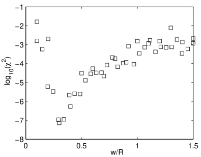
Figure 3: $\chi^{2}$ error of the reconstructed vortex field after 100 iterations as a function of the width $w$ of $V$.

Several stages of the reconstruction algorithm are shown in figures 4(b)-(d). (The field reconstruction in this example takes about 30 minutes on a Pentium 4 CPU and uses approximately 400 MB of memory.) We show only the real part of the field, as the imaginary part shows a similar degree of agreement. The XFROG error $Z$ of Eq. (8) for the same simulation run is shown in Fig. 5 as a function of the number of iterations. Also shown is the deviation from the reconstructed field from the original field $\chi^{2}$. The figure shows that the algorithm converges exponentially after some initial stagnation. It also shows that, after the ambiguity in the total phase has been taken into account, the XFROG error $Z$ is a good measure of the actual discrepancy between reconstructed and original field. This is important for real-life applications since in practice one does not know the original field so that $\chi^{2}$ cannot be calculated and only the XFROG error is accessible.

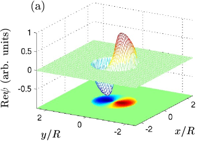
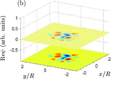
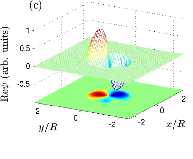
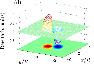
Figure 4: (Color online) Reconstruction of a vortex state on a grid of $64\times 64$ points. Figure (a) shows the real part of the original state and figures (b)-(d) show the initial guess and the reconstructed state after 50 and 100 iterations, respectively.

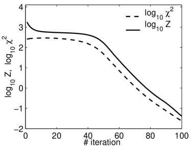
Figure 5: FROG error $Z$ and field error $\chi^{2}$ for the simulation run of Fig. 4.

Time of flight absorption imaging is a comparatively easy way to obtain many data points in the Fourier domain, but it is cumbersome to obtain the data sets for different shifts ${\bf{R}}$ because each such set requires a new run of the experiment. Thus a natural question is the sensitivity of the algorithm to the number of displacements for which a measurement is performed.

To answer this question we have calculated XFROG signals $I_{\rm XFROG}$ on grids of dimension $n\times n$, interpolated them onto a larger grid of dimension $N\times N$ using cubic splines, and applied the XFROG algorithm to the resulting XFROG signals. Fig. 6 shows an example for $n=10$. The recovered field shows good agreement with the original field, with differences in some details, e.g. near the maxima, resulting from the smoothing property of the interpolation with splines.

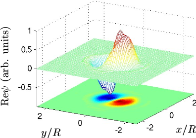
Figure 6: (Color online) Reconstruction of the field of Fig. 4 with the XFROG signal simulated on a grid of $10\times 10$ and interpolated on a grid of $64\times 64$ after 100 iterations.

To quantitatively characterize the dependence of the success of the field recovery on the number of measurements we have evaluated $\chi^{2}$ of the recovered field after 100 iterations as a function of $n$. The result is shown in Fig. 7. While the discrepancy between the recovered field and the original field grows as expected as the number of measurements decreases, the field is qualitatively retrieved down to $n=7$. For even smaller $n$ the field reconstruction fails. In those cases the algorithm is honest enough to admit its failure by generating a large residual XFROG error. Nonetheless, the conclusion is that a rather limited number of measurements is sufficient to accurately measure the field.

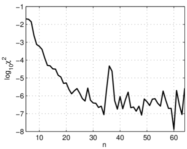
Figure 7: $\chi^{2}$ error of the recovered field after 100 iterations as a function of the number of measured data points $n$ (same parameters as in figures 4 and 5).

We remark that these considerations are actually overly pessimistic. In reality one often knows the size of the atomic cloud and the XFROG signal is clearly zero if there is no overlap between coupling $V$ and atomic field $\psi$. Thus, many data points in the XFROG signal can be padded with zeros. Even those zeros contain usable information for the XFROG algorithm because they encode a support constraint for the recovered field. Support constraints, together with Fourier domain information, are widely used in image reconstruction for astronomic imagery and under certain circumstances they characterize an image completely. Furthermore, among the remaining non-zero measurements some will give excessively small signals. In practice one can replace these measurements by other displacements that give a stronger signal.

In an actual experiment the measurement of an XFROG signal will be subject to several sources of noise. In that case the intersection of the sets $O$ and $F$ in Fig. 2 will in general be empty, and the XFROG algorithm determines a field that has the correct XFROG signal, i.e. belongs to the set $F$, and at the same time minimizes the distance to the set $O$ as measured by $Z$.

The XFROG signal Eq. (8) is insensitive to fluctuations in the total phase of the atomic field $\psi$ from one run of the experiment to the other, i.e. for different ${\bf{R}}$ — a consequence of the non-interferometric character of FROG methods in general. Hence it is sufficient to study the impact of uncertainties in the measurement of the displacements ${\bf{R}}$ themselves and in the total intensity of the XFROG signal from shot to shot. The latter can arise from variations of the number of atoms in the original condensate, from fluctuations in the coupling strength, and from fluctuations in the interaction times. We have simulated XFROG signals with Gaussian fluctuations in ${\bf{R}}$ and in shot-to-shot total intensity $I$ with variances $\Delta{\bf{R}}$ and $\Delta I$, respectively. Note that with our choice of normalization for $\psi$ and $V$ the total intensity of the XFROG signals is of order one so that we can treat absolute errors and relative errors in $I$ as being the same.

We have applied the XFROG algorithm to these contaminated signals and we have measured $\chi^{2}$ after 100 iterations. To be more realistic, we have simulated the XFROG signals only on a grid of $10\times 10$ and interpolated onto a grid of $64\times 64$ as above. We have simulated the situation with errors in ${\bf{R}}$ only, errors in $I$ only, and errors in both ${\bf{R}}$ and $I$. The results are summarized in Fig. 9. We were able to qualitatively reconstruct the atomic field up to relative errors as large as $\Delta R/R\approx 0.3$ and $\Delta I/I=1$. The algorithm was found to be significantly less sensitive to uncertainties in the total intensity than to uncertainties in the displacements. Even XFROG signals with $\Delta I/I=1$ yield recovered fields of very high quality. The relatively high residual errors for $\Delta I/I\approx 0.4$ and $\Delta I/I\approx 0.8$ come about because the XFROG algorithm did not find the global minimum of $Z$ for the particular initial guess. Restarting the algorithm with a different initial guess (but with the exact same contaminated XFROG signal) lead to residual errors that nicely interpolate the the other data points.

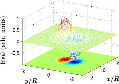
Figure 8: (Color online) Same as Fig. 6 but with simulated noise $\Delta R/R=0.1$ and $\Delta I/I=0.1$ in the XFROG signal.

Figure 8 shows the retrieved field after 100 iterations for $\Delta R/R=0.11$ and $\Delta I/I=0.11$. The broad features of the original field are clearly reproduced and the noisy fine structure is exclusively due to the fluctuations in ${\bf{R}}$ and could be smoothed out by convolution with a Gaussian of width comparable to the healing length. Thus, although the error in the retrieved field increases with increasing noise, we conclude that the algorithm is not very sensitive to noise and yields at least reliable qualitative information. In a sense, the field as recovered by the XFROG method contains much less noise than the input data. This is reminiscent of the situation encountered in image reconstruction e.g. in astronomical applications. And it was exactly for the purpose of removing noise from images by using a mixture of position space and Fourier space information that many of the methods described in this paper were first discussed.

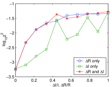
Figure 9: (Color online) $\chi^{2}$ error of the recovered field after 100 iterations as a function of several noise sources.

In summary we have shown how the powerful XFROG method of ultrafast optics can be adapted to phase measurement applications in ultra-cold atomic systems. In particular, this technique is capable of correctly recovering a vortex state and it is robust against noise, with a number of actual measurements that can be reduced to experimentally feasible values.

An interesting question for the future is how the XFROG method can be used to study situations were there is no well defined phase of the atomic field for fundamental reasons. For example the XFROG technique could be a valuable tool for diagnosing the transition of an elongated BEC (with long range phase coherence) to a quasi one-dimensional Tonks-Girardeau gas (without phase coherence), or the transition of a rapidly rotating BEC into the quantum Hall regime. The XFROG method could also be of interest in the study of the so-called BCS-BEC crossover where a superfluid of Cooper pairs goes over into a BEC of tightly bound molecules.

We thank H. Giessen for valuable criticism on the manuscript. This work has been supported in part by the US Office of Naval Research, by the National Science Foundation, by the US Army Research Office, and by the National Aeronautics and Space Administration.

References

- Davis et al. (1995) K. Davis, M. O. Mewes, M. R. Andrews, N. J. van Druten, D. S. Durfee, D. M. Kurn, and W. Ketterle, Phys. Rev. Lett. 75, 3969 (1995).
- Bradley et al. (1995) C. C. Bradley, C. A. Sackett, J. J. Tollett, and R. G. Hulet, Phys. Rev. Lett. 75, 1687 (1995).
- Anderson et al. (1995) M. H. Anderson, J. R. Ensher, M. R. Mathews, C. E. Wieman, and E. E. Cornell, Science 269, 198 (1995).
- Ketterle and H.-J. Miesner (1997) W. Ketterle and H.-J. Miesner, Phys. Rev. A 56, 3291 (1997).
- Andrews et al. (1997) M. R. Andrews, C. G. Townsend, H.-J. Miesner, D. S. Durfee, D. M. Kurn, and W. Ketterle, Science 275, 637 (1997).
- Ketterle et al. (1999) W. Ketterle, D. S. Durfee, and D. M. Stamper-Kurn, in Bose-Einstein condensation in atomic gases, edited by M. Inguscio, S. Stringari, and C. E. Wieman, Proceedings of the International School of Physics ”Enrico Fermi”, Course CXL (IOS Press, Amsterdam, 1999), pp. 67–176, eprint cond-mat/9904034.
- You et al. (1996) L. You, M. Lewenstein, R. J. Glauber, and J. Cooper, Phys. Rev. A 53, 329 (1996).
- You and Lewenstein (1996) L. You and M. Lewenstein, J. Res. Natl. Inst. Stand. Technol. 101, 575 (1996).
- Politzer (1995) H. D. Politzer, Phys. Lett. A 209, 160 (1995).
- Politzer (1997) H. D. Politzer, Phys. Rev. A 55, 1140 (1997).
- Matthews et al. (1999) M. R. Matthews, B. P. Anderson, P. C. Haljan, D. S. Hall, C. E. Wieman, and E. A. Cornell, Phys. Rev. Lett. 83, 2498 (1999).
- J. L. A. Chilla and O. E. Martinez (1991) J. L. A. Chilla and O. E. Martinez, Opt. Lett. 16, 39 (1991).
- Kane and Trebino (1993a) D. J. Kane and R. Trebino, IEEE J. Quantum Electron. 29, 571 (1993a).
- DeLong et al. (1994) K. W. DeLong, R. Trebino, J. Hunter, and W. E. White, J. Opt. Soc. Am. B 11, 2206 (1994).
- Trebino and Kane (1993) R. Trebino and D. J. Kane, J. Opt. Soc. Am. A 10, 1101 (1993).
- Kane and Trebino (1993b) D. J. Kane and R. Trebino, Opt. Lett. 18, 823 (1993b).
- Trebino et al. (1997) R. Trebino et al., Rev. Sci. Instrum. 68, 3277 (1997).
- Trebino (2000) R. Trebino, ed., Frequency-resolved optical gating: the measurement of ultrashort laser pulses (Kluver, Boston, 2000).
- Linden et al. (1999) S. Linden, J. Kuhl, and H. Giessen, Opt. Lett. 24, 569 (1999).
- Linden et al. (1998) S. Linden, H. Giessen, and J. Kuhl, Phys. Stat. Sol. (b) 206, 119 (1998).
- Linden et al. (2000) S. Linden, J. Kuhl, and H. Giessen, in Frequency-resolved optical gating: the measurement of ultrashort laser pulses, edited by R. Trebino (Kluver, Boston, 2000), pp. 313–322.
- Fienup (1982) J. R. Fienup, Appl. Opt. 21, 2758 (1982).
- Yudilevich et al. (1987) E. Yudilevich, A. Levi, G. J. Habetler, and H. Stark, J. Opt. Soc. Am. A 4, 236 (1987).
- DeLong and Trebino (1994) K. W. DeLong and R. Trebino, J. Opt. Soc. Am. A 11, 2429 (1994).
- Kenneth W. DeLong et al. (1994) Kenneth W. DeLong et al., Opt. Lett. 19, 2152 (1994).
- Wynar et al. (2000) R. Wynar et al., Science 287, 1016 (2000).
- Inouye et al. (1998) S. Inouye et al., Nature (London) 392, 151 (1998).
- Donley et al. (2002) E. A. Donley, N. R. Claussen, S. T. Thompson, and C. E. Wieman, Nature (London) 417, 529 (2002).
- Dürr et al. (2004) S. Dürr, T. Volz, A. Marte, and G. Rempe, Phys. Rev. Lett. 92, 020406 (2004).
- Greiner et al. (2003) M. Greiner, C. A. Regal, and D. S. Jin, Nature (London) 426, 537 (2003).
- Jochim et al. (2003) S. Jochim et al., Science 302, 2101 (2003).
- Pethick and Smith (2002) C. J. Pethick and H. Smith, Bose-Einstein condensation in dilute gases (Cambridge University Publications, 2002).