The Truncated Polynomial Expansion Monte Carlo Method for Fermion Systems Coupled to Classical Fields: A Model Independent Implementation

Abstract

A software library is presented for the polynomial expansion method (PEM) of the density of states (DOS) introduced in Ref re:motome99 , re:furukawa01 . The library provides all necessary functions for the use of the PEM and its truncated version (TPEM) in a model independent way. The PEM/TPEM replaces the exact diagonalization of the one electron sector in models for fermions coupled to classical fields. The computational cost of the algorithm is $O(N)$ – with $N$ the number of lattice sites – for the TPEMre:furukawa03 which should be contrasted with the computational cost of the diagonalization technique that scales as $O(N^{4})$. The method is applied for the first time to a double exchange model with finite Hund coupling and also to diluted spin-fermion models.

, , , and

PROGRAM SUMMARY

(Computer program available on request)
Title of library: TPEM
Distribution Format: tar gzip file
Operating System: Linux, UNIX
Number of Files: 4 plus 1 test program
Keywords: Moment expansion, Monte Carlo method, Correlated electrons
Programming language used: C
Computer: PC
Typical running time: The test program takes a few seconds to run.
External routines: The LaPack library can be used by the test program and the GSL library can be used by TPEM though they are not essential.
Nature of the physical problem: The study of correlated electrons coupled to classical fields appears in the treatment of many materials of much current interest in condensed matter theory, e. g. manganites, diluted magnetic semiconductors and high temperature superconductors among others.
Method of solution: Typically an exact diagonalization of the electronic sector is performed in this type of models for each configuration of classical fields, which are integrated using a classical Monte Carlo algorithm. A polynomial expansion of the density of states is able to replace the exact diagonalization, decreasing the computational complexity of the problem from $O(N^{4})$ to $O(N)$ and allowing for the study of larger lattices and more complex and realistic systems.
Key References: re:motome99 , re:furukawa03 , re:dagotto02 , re:alvarez02 .

1 Introduction

The problem of fermions coupled to classical fields appears in many contexts in condensed matter physics. In this kind of problems the fermionic operators appear in the Hamiltonian involving only quadratic terms. They can be solved re:dagotto02 by diagonalizing the fermions exactly in the one-electron sector at finite temperature for a given configuration of classical fields. The classical fields are integrated by means of a classical Monte Carlo algorithm. The procedure, apart from being exact within the error bars, preserves the lattice throughout the calculation making it possible to study the spatial dependence of the observables. This is a crucial issue to understand inhomogeneities and has been successfully applied to the study of many materials re:alvarez04 . In the case of manganites such models have been used to understand the phase diagram of these materials as well as the colossal magnetoresistance effect re:dagotto02 , i. e. the colossal response of the system to magnetic fields, that could have many important applications. In this case, the classical field is the local $t_{2g}$ spin. Diluted magnetic semiconductors have also been studied in a similar way re:alvarez02 . The inhomogeneities that appear there in the form of ferromagnetic clusters, could only be accessed by the use of this method re:alvarez03 . In addition, a model for high temperature superconductors has been presented re:alvarez04b to study the competition between d-wave superconductivity and antiferromagnetism that seems to explain interesting properties of these complex materials.
Despite all these many advantages of the method, it is still very costly in terms of computational effort. Indeed, the method scales as order $O(N^{4})$ and the largest lattices that can be accessed in a practical way contain no more than $6^{3}$ sites or its equivalent in lower dimensions. This imposes limitations on the kind of physical systems that can be studied, for example, the Mn spin concentration in diluted semiconductors has to be high enough, the study of many band systems becomes difficult, etc.
Trying to solve some of these problems, two of the authors (N.F. and Y.M.) proposed re:motome99 , re:furukawa01 in 2001 a procedure that replaces the exact diagonalization of the one-electron sector by a series expansion of the density of states in terms of Chebyshev polynomials. The method takes advantage of the sparseness of the Hamiltonian matrix (which is the case in virtually all systems of physical interest) to perform the matrix-vector products that appear in the calculation of the terms or moments of the expansion. In what follows, this method will be referred to as the polynomial expansion method or PEM. In 2003 an improvement of the PEM was proposed, re:furukawa03 based on two controllable approximations that, as will be seen, do not diminish in any way the quality of the results. The first of these approximations is the truncation of each matrix-vector multiplication, including only products that are larger than a certain threshold. The second one is the truncation of the difference in Boltzmann probability weight or action between two very similar configurations of classical fields. This difference appears in the Monte Carlo procedure with enormous frequency and so its truncation turns out to be very effective. This new truncated PEM will be referred to as TPEM.
In this paper we present a C library that implements both the PEM and TPEM. The library is model independent and basically takes as input the Hamiltonian matrix of practically any model of fermions coupled to classical fields. To our knowledge no such library is presently available but its usefulness is evident: the TPEM can be easily separated from other details of the main program(s) and users do not have to be concerned with the technicalities of the method. In this sense the library presented here places the TPEM at the same level of the exact diagonalization.
Another algorithm for the study of spin-fermion models on large lattices is the “Hybrid Monte Carlo Algorithm”, that has been applied to the double-exchange model with infinite coupling re:alonso01 . In this method the model is formulated in the path integral representation, introducing imaginary time, and a Hybrid Monte Carlo (HMC) procedure is used to evolve the system. The TPEM seems to work best than the HMC at low temperature where the HMC presents increasing computational cost due to the time discretization. Furthermore, the HMC is applicable when the bands are connected and do not extend over a wide range of energies, as is the case of finite coupling systems. The TPEM also allows for easy parallelization, improving the performance even more.
The paper is divided as follows. Section 2 explains the theory underlying the TPEM. In Section 3 the implementation details and the functions provided by the library are described. Section 4 shows some simple examples on how to use the library. Finally, in Section 5, the TPEM is applied to a model for manganites with finite coupling and also to diluted spin-fermion systems.
It is important to emphasize that the application of the TPEM to finite Hund coupling and diluted systems is novel and shows that the method is suitable to study both systems with disconnected bands and systems with impurity bands.

2 Theoretical Overview

The analysis starts with a model defined by a certain Hamiltonian, $\hat{H}=\sum_{ij\alpha\beta}c^{\dagger}_{i\alpha}H_{i\alpha,j\beta}(\phi)c_{j\beta}$, where the indices $i$ and $j$ denote a spatial index and $\alpha$ and $\beta$ some internal degree(s) of freedom, e. g. spin or orbital. The Hamiltonian matrix depends on the configuration of one or more classical fields, represented by $\phi$. Although no explicit indices will be used, the field(s) $\phi$ are supposed to have a spatial dependence. The partition function for this Hamiltonian is given by:

$$Z=\int d\phi\sum_{n}\langle n|\exp(-\beta\hat{H}(\phi)+\beta\mu\hat{N})|n\rangle$$ (1)

where $|n\rangle$ are the eigenvectors of the one-electron sector. To calculate the observables, an arbitrary configuration of classical fields $\phi$ is selected as a starting point. The Boltzmann weight or action of that configuration, $S(\phi)$, is calculated by diagonalizing the one-electron sector at finite temperature. Then a small local change of the field configuration is proposed, so that the new configuration is denoted by $\phi^{\prime}$ and its action is recalculated to obtain the difference in action $\Delta S=S(\phi^{\prime})-S(\phi)$ . This new configuration is accepted or rejected based on a Monte Carlo algorithm like Metropolis or heat bath and the cycle starts again. In short, the observables are traditionally calculated using exact diagonalization of the one-electron sector at every spin “flip” and Monte Carlo integration for the classical fields re:dagotto02 . The PEM/TPEM substitutes the diagonalization for a polynomial expansion and the details are presented in Ref. re:motome99 , re:furukawa01 , re:furukawa03 .
It will be assumed that the Hamiltonian $H(\phi)$ is normalized, which simply implies a re-scaling:

$$H \rightarrow (H-b)/a$$

$$a = (E_{max}-E_{min})/2$$

$$b = (E_{max}+E_{min})/2,$$ (2)

where $E_{max}$ and $E_{min}$ are the maximum and minimum eigenvalues of the original Hamiltonian respectively. This in turn implies that the normalized Hamiltonian has eigenvalues $\epsilon_{v}\in[-1,1]$. The values of $E_{max}$ and $E_{min}$ depend on the particular Hamiltonian under consideration and should be calculated in advance.
The observables that can be calculated directly with the TPEM fall into two categories: (i) those that do not depend directly on fermionic operators, e. g. the magnetization, susceptibility and classical spin-spin correlations in the double exchange model and (ii) those for which a function $F(x)$ exists such that they can be written as:

$$A(\phi)=\int_{-1}^{1}F(x)D(\phi,x)dx,$$ (3)

where $D(\phi,\epsilon)=\sum_{\nu}\delta(\epsilon(\phi)-\epsilon_{\nu})$, and $\epsilon_{\nu}$ are the eigenvalues of $H(\phi)$, i. e. $D(\phi,x)$ is the density of states of the system. For the former, the calculation is straightforward and simply involves the average over Monte Carlo configurations. For the latter, a function $F(x)$ can be expanded in terms of Chebyshev polynomials in the following way:

$$F(x)=\sum_{m=0}^{\infty}f_{m}T_{m}(x),$$ (4)

where $T_{m}(x)$ is the $m-$th Chebyshev polynomial evaluated at $x$. Let $\alpha_{m}=2-\delta_{m,0}$. The coefficients $f_{m}$ are calculated using the formula:

$$f_{m}=\int_{-1}^{1}\alpha_{m}F(x)T_{m}(x)/(\pi\sqrt{1-x^{2}}).$$ (5)

The moments of the density of states are defined by:

$$\mu_{m}(\phi)=\sum_{\nu=1}^{N_{dim}}\langle\nu|T_{m}(H(\phi))|\nu\rangle,$$ (6)

where $N_{dim}$ is the dimension of the one-electron sector. Then, the observable corresponding to the function $F(x)$, can be calculated using:

$$A(\phi)=\sum_{m}f_{m}\mu_{m}(\phi)$$ (7)

In practice, the sum in Eq. (7) is performed up to a certain cutoff value $M$, without appreciable loss in accuracy as described in Ref. re:motome99 , re:furukawa01 . The calculation of $\mu_{m}$ is carried out recursively. $|\nu;m\rangle=T_{m}(H)|\nu\rangle=2H|\nu;m-1\rangle-|\nu;m-2\rangle$ and hence:

$$\mu_{2m} = \sum_{\nu}(\langle m;\nu|\nu;m\rangle-1)$$

$$\mu_{2m+1} = \sum_{\nu}(\langle m;\nu|\nu;m\rangle+1-\langle\nu;0|\nu;1\rangle),$$ (8)

are used to calculate the moments. The process involves a sparse matrix-vector product, e. g. in $T_{m}(H)|\nu\rangle$, yielding a cost of $O(N^{2})$ for each configuration, i. e. $O(N^{3})$ for each Monte Carlo step. In addition, an improvement of the present method has been proposed re:furukawa03 based on a truncation of the matrix-vector product mentioned before and it turns out that the resulting algorithm has a complexity linear in $N$. This approximation is controlled by the small parameter $\epsilon_{pr}$.
Moreover, for the Monte Carlo integration procedure, the difference in action, $\Delta S=S(\phi^{\prime})-S(\phi)$ has to be computed at every step. Since this operation requires calculating two set of moments, for $\phi$ and $\phi^{\prime}$, the authors of Ref. re:furukawa03 have also developed a truncation procedure for this trace operation controlled by a small parameter, $\epsilon_{tr}$. This truncation is based on the observation that if $\phi$ and $\phi^{\prime}$ differ only in very few sites then the corresponding moments will differ only for certain indices allowing for a significant reduction of the computational complexity. The TPEM library presented here implements this truncation as well.
In what follows, the size of the Hilbert space will be denoted by $N_{dim}$ and it will depend on the size of the lattice as well as on the particular model to be studied. For a one-band double exchange model on a lattice of $N$ sites and finite coupling, $N_{dim}=2N$; the factor of 2 accounts for the spin degree of freedom.

3 The Library

3.1 Implementation

The code is written in C and can be called from a C or C++ program. If the library is compiled statically the file libtpem.a is produced. To use the functions provided by the library the header file “tpem.h” has to be included.
In the code, complex numbers are simply represented by the structure:
typedef struct { double real, imag; } tpem_t;
As mentioned before, matrix-vector multiplications must be performed in a sparse way, i. e., multiplications that yield a null result must be avoided for efficiency. The structure tpem_sparse, defined in tpem_sparse.c, implements a sparse matrix in compressed row storage (CRS) format. The CRS format puts the subsequent nonzero elements of the matrix rows in contiguous memory locations. We create 3 vectors: one for complex numbers containing the values of the matrix entries and the other two for integers ($colind$ and $rowptr$). The vector $values$ stores the values of the non-zero elements of the matrix, as they are traversed in a row-wise fashion. The $colind$ vector stores the column indices of the elements of the $values$ vector. That is, if $values[k]=a[i][j]$ then $colind[k]=j$. The $rowptr$ vector stores the locations in the $values$ vector that start a row, that is $values[k]=a[i][j]$ if $rowptr[i]\leq i<rowptr[i+1]$. By convention, we define $rowptr[N_{dim}]$ to be equal to the number of non-zero elements, $n_{z}$, in the matrix. The storage savings of this approach are significant since instead of storing $N_{dim}^{2}$ elements, we need only $2n_{z}+N_{dim}+1$ storage locations.
To illustrate how the CRS format works, consider the non-symmetric matrix defined by

$$A=\left[\begin{tabular}[]{llllll}10&0&0&0&-2&0\\ 3&9&0&0&0&3\\ 0&7&8&7&0&0\\ 3&0&8&7&5&0\\ 0&8&0&9&9&13\\ 0&4&0&0&2&-1\\ \end{tabular}\right]$$ (9)

The CRS format for this matrix is then specified by the arrays:
values = [10 -2 3 9 3 7 8 7 3 ... 9 13 4 2 -1 ]
colind = [ 0 4 0 1 5 1 2 3 0 ... 4 5 1 4 5 ]
rowptr = [ 0 2 5 8 12 16 19 ]
Besides the obvious saving in storage, CRS format allows for a model independent library implementation and an easy algorithm for matrix-vector multiplication as shown in Fig. 1.

     void tpem_sparse_mult (sparse *matrix, tpem_t *dest,  tpem_t *src)  {    size_t row, col, k;    tpem_t tmp;      for (row = 0; row < matrix->rank; row++) {      sum = 0.0;      for (k=matrix->rowptr[row];k<matrix->rowptr[row+1];k++) {        col  = matrix->colind[k];        sum += matrix->values[k] * src[col];      }      dest[row] = sum;    }  }     

Figure 1: Matrix-vector multiplication function using the CRS format. $src$ contains the vector to be multiplied and the results are stored in $dest$.

The truncations in the matrix-vector product and in the action difference are calculated with the aid of tpem_subspace.c which implements a simple stack. The stack is used to hold a “subspace” of kets of the one-electron Hilbert space that grows dynamically. It is in this subspace that matrix-vector multiplications are performed instead of using the complete Hilbert space.

3.2 Functions provided by the Library

1. void tpem_init();

Description: It must be called before using the library.

2. void tpem_calculate_coeffs (size_t M, double *coeffs,
double (*G)(int,double));

Description: It calculates $f_{m}$ using Eq. (5).

Arguments:

• M: cutoff (input)

• coeffs: array of doubles where the coefficients $f_{m}$, Eq. (4) will be stored. (output)

• double (*F)(double): The function corresponding to the observable that we want to expand as given by Eq. (3). The function takes a double and returns a double (input).

3. void tpem_calculate_moment_tpem (tpem_sparse *matrix, size_t M, double *moment,double epsProd);

Description: It calculates the moments of the density of states, $\mu_{m}$, as defined by Eq. (6). The method used is TPEM as described in re:furukawa03 .

Arguments:

• matrix: the matrix in compressed row storage (input).

• M: the cutoff (input).

• moment: array of doubles to store the moments, Eq. (6) (output).

• epsProd: the tolerance for the matrix-vector product truncation (input).

4. void tpem_calculate_moment_pem (tpem_sparse *matrix, size_t M, double *moment);

Description: Same as previous but it uses PEM algorithm.

void tpem_calculate_moment_diff_tpem (tpem_sparse *matrix0, tpem_sparse *matrix1, size_t M, double *moments, size_t n_support, size_t *support, double epsTrace, double epsProd);

Description: It calculates the difference in moments for two matrices, using the trace truncation algorithm.

Arguments:

• matrix0: The first matrix (input).

• matrix1: The second matrix (input).

• M: the cutoff (input).

• moments: array of doubles to store the difference in moments (output).

• n_support: Number of entries where the two matrices differ (input).

• support: Vector containing the column index of the entries where the two matrices differ. For example, in the double exchange model with finite coupling if site $i$ is being updated then support=[i,i+N] where N is the number of sites (input).

• epsTrace: The tolerance for the trace truncation algorithm (input).

• epsProd: The tolerance for the matrix-vector multiplication truncation (input).

Note that this function does not calculate the moment difference for any two matrices, only for matrices that differ in indices specified by n_support and support as explained above.

5. void tpem_calculate_moment_diff_pem (tpem_sparse *matrix0, tpem_sparse *matrix1, size_t M, double *moments);

Description: It calculates the difference in moments for two matrices without approximations. This function is provided for easy integration of PEM and TPEM algorithms. Since there is no truncation, the support array, its size and the tolerances are not needed.

6. double tpem_expansion (size_t M, double *moments, double *coeffs)

Description: Given $f_{m}$ and $\mu_{m}$ calculates $A(\phi)$ as given by Eq. (7).

7. void tpem_finalize();

Description: It can be called to free the resources used by the library and reset all input.

4 Simple Examples

4.1 Calculating an Integral

To illustrate the use of the library several integrals will be calculated based on a density of states, $D(x)$, given by the one-dimensional spinless double exchange model with random potentials, $V_{i}$, whose Hamiltonian is:

$${\hat{H}}=-t\sum_{<ij>,\sigma}{\hat{c}}^{\dagger}_{i\sigma}{\hat{c}}_{j\sigma}+\sum_{i}V_{i}\hat{n}_{i}.$$ (10)

The complete code discussed in this section is provided in the file tpem_test.c. The most important steps will be explained here. The matrix used is $400\times 400$, is calculated in the CRS format and normalized so that its eigenvalues are in the interval $[-1,1]$ as explained in Section 2 and in Eq. (2). The library must be initialized by calling the function tpem_init. Let us define $E(x)=5.0x(1.0-\tanh(10.0x))$ and calculate $\int_{-1}^{1}D(x)E(x)dx$ applying both exact diagonalization and the TPEM. In tpem_test.c the diagonalization is done by calling the function diag_apply. Next the integral is performed using the TPEM for different values of the cutoff, $M$, and fixed $\epsilon_{pr}=10^{-5}$ and $\epsilon_{tr}=10^{-3}$ in the function tpem_apply. The code is self explanatory and shows the ease of use of the library: First, the coefficients need to be calculated using:
tpem_calculate_coeffs (cutoff, coeffs, funcptr);
Next, the moments are obtained by calling:
tpem_calculate_moment_tpem(matrix, cutoff, moment,eps);
Finally, the integral is calculated simply by multiplying the moments times the coefficients: ret = tpem_expansion (cutoff, moment, coeffs);
The output of the program is presented at the end and in Fig. 2a.

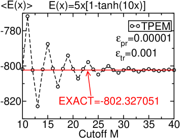
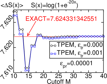
Figure 2: (a) $\langle E(x)\rangle$ calculated using the TPEM with the parameters shown vs. the cutoff, $M$. The exact value is also indicated. (b) $\langle\Delta S(x)\rangle$ calculated using the TPEM with and without trace truncation vs. the cutoff, $M$. In the former case $\epsilon_{tr}=0.001$ and in the latter $\epsilon_{tr}=0$. The exact value is also indicated.

Similarly, other integrals are calculated in tpem_test.c with the function $N(x)=0.5(1.0-\tanh(10.0x))$. In both cases, it can be seen that after $M\approx 30$ the results agree with the ones obtained by applying the traditional diagonalization method. Moreover, if only $M$ even is considered then the convergence for $E(x)$ is achieved for a much smaller value of $M$, namely $M\approx 10$.

4.2 Using Trace Truncation

The last part of tpem_test.c tests the trace truncation. Consider two matrices corresponding to a one-dimensional spinless double exchange model with random potentials, Eq. (10), that differ only in the value of the potential at the first site. Consider the function, $S(x)=\log(1.0+\exp(-10.0x))$, which emulates the action. The testing program calculates the difference in $S(x)$ for both matrices in three ways: (i) with the exact diagonalization, (ii) by using the TPEM without trace truncation and (iii) by using trace truncation. The last two results are parameterized in terms of $M$ and both assume $\epsilon_{pr}=10^{-5}$ whereas $\epsilon_{tr}=0$ when no trace truncation is used and $\epsilon_{tr}=10^{-3}$ in the second case.
The results are presented in Fig. 2b. Both TPEM calculations agree with the exact diagonalization after $M\approx 20$.

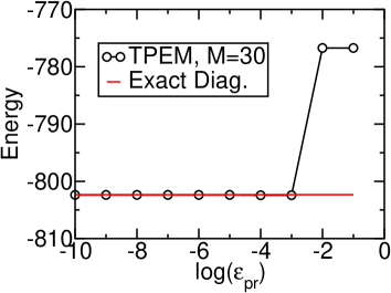
Figure 3: TPEM calculated $\langle E\rangle$ for different values of $\epsilon_{pr}$. The $x-$axis is given in logarithmic scale. The value of $\langle E\rangle$ from the exact diagonalization technique is also indicated.

The dependence of the quality of the results on $\epsilon_{pr}$ is shown in Fig. 3 for the function $E(x)$ where it can be seen that $\epsilon_{pr}=10^{-3}$ is enough to obtain very high accuracy for this model. However, for the systems that will be described in the next section we have found that $\epsilon_{pr}$ should be as small as $10^{-5}$ for the results to be accurate, and this value will be used in the rest of this work.

5 Advanced Applications: TPEM and Monte Carlo

5.1 Double Exchange Model at Finite Coupling

Double exchange models appear in the description of the colossal magnetoresistance effect (CMR) in manganites where the electron-phonon coupling and the Coulomb interactions are usually neglectedre:dagotto01 . These models can correctly produce ferromagnetic phases as long as the Hund coupling is large enough. In this case, the electrons directly jump from manganese to manganese spin and their kinetic energy is minimized if these spins are aligned. The Hamiltonian of the system in the one-band approximation can be written as re:zener52 , re:furukawa94 :

$${\hat{H}}=-t\sum_{<ij>,\sigma}{\hat{c}}^{\dagger}_{i\sigma}{\hat{c}}_{j\sigma}-J\sum\vec{S}_{i}\cdot\vec{\sigma}_{i},$$ (11)

where ${\hat{c}}^{\dagger}_{i\sigma}$ creates a carrier at site $i$ with spin $\sigma$. The carrier-spin operator interacting ferromagnetically with the localized Mn-spin $\vec{S}_{i}$ is $\vec{\sigma}_{i}=\sum_{\alpha,\beta}{\hat{c}}^{\dagger}_{i\alpha}\vec{\sigma}_{\alpha,\beta}{\hat{c}}_{i\beta}$. On a cubic lattice of dimension $D$ the largest and smallest spectrum bounds of Hamiltonian Eq. (11) are $E_{min}=-2tD-J$ and $E_{max}=-2tD+J$, respectively. To test the TPEM for this physical model, we start with the interesting case of a ferromagnetic to paramagnetic transition. The coupling $J$ is chosen to be $J=8t$ and the electronic density is adjusted with $\mu=-8t$ to obtain a quarter filling, i. e. $n=0.5$. We have performed 1,000 thermalization and 1,000 measurements which were enough to achieve both convergence and small errors. The results for the magnetization of the system, defined as

$$|M|=\frac{1}{N}|\sum_{i}\vec{S}_{i}|$$ (12)

are shown in Fig. 4 and compared to the traditional exact diagonalization calculation, where the high accuracy of the method can be seen clearly.

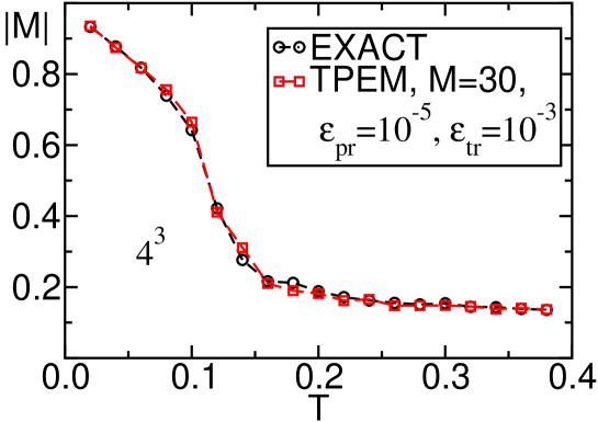
Figure 4: Magnetization vs. temperature, $T$, on a $4^{3}$ lattice for model Eq. (11), calculated using both exact diagonalization and the TPEM with the indicated parameters. The maximum possible value of $|M|$ is 1.

We repeat the calculations for larger lattices and also measure the magnetic susceptibility, $\chi$, as a function of the temperature (see Fig. 5).
The boundary conditions used are anti-periodic in one direction and periodic in the other two. This is a numerical trick in the sense that it is an effective way to lift the degeneracy due to small size lattices. This degeneracy affects the form of the density of states making it difficult to expand it when performing simulations on $4^{3}$. The effect is less and less relevant as size increases. Moreover, the choice of boundary conditions does not matter in the thermodynamic limit. Twisted boundary conditions has been used extensively in numerical simulations re:assaad02 , re:nakano99 .

The CPU times to perform these computations are shown in Fig. 6a making use of a conventional cluster of linux PCs with 3.06GHz of clock frequency each. Even using commodity PCs the CPU user time to perform calculations on the largest cluster studied, $10^{3}$, was less than 3 days. The results show that the CPU time scales linearly with the size of the system as predicted by the theory re:furukawa03 . Moreover, the algorithm can be parallelized. This is because calculation of the moments in Eq. (6) is completely independent for each basis ket $|\nu\rangle$. In this way the basis can be partitioned in such a way that each processor calculates the moments corresponding to a portion of the basis. The CPU time to calculate the moments on each processor is proportional to $N_{dim}/N_{PE}$, where $N_{PE}$ is the number of processors. It is important to remark that the data to be moved between different nodes are small compared to calculations in each node, the communication time is proportional to $MN_{PE}$. Communication among nodes is mainly done here to add up all the moments. A version of the TPEM library that supports parallelization will be available in the future.

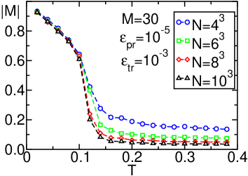
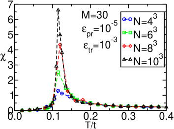
Figure 5: TPEM calculated (a) Magnetization vs. $T$ and (b) $\chi$ vs. $T$ for the lattices and parameters indicated.

The value of $T_{\rm C}$ obtained from the $\chi$ vs. $T$ curves is approximately $T_{\rm C}=0.12t$ at $J=8t$ in very good agreement with previously calculated values re:motome00 , re:yunoki98 . In addition, we calculated the scaling coefficient $\beta$ defined by $|M|\propto(T_{C}-T)^{\beta}$, after having made a size-extrapolation, i. e., after taking the thermodynamic limit. The result is shown in Fig. 6b and is within the error margin of the value given for the Universality class of the Heisenberg model. More information about the determination of critical exponents can be found in Ref. re:pelissetto02 .

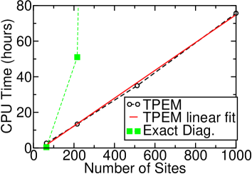
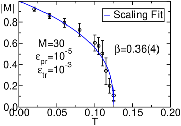
Figure 6: (a) CPU Times for the TPEM algorithm applied to model Eq. (11) using 2,000 Monte Carlo steps, $M=30$, $\epsilon_{pr}=10^{-5}$, $\epsilon_{tr}=10^{-3}$ on a 3.06GHz PC. The linear fit yields $y=0.0782x-3.3271$. The CPU times required for the exact diagonalization procedure are also shown. (b) $|M|$ vs. $T$ for size-extrapolated data (lattices used: $4^{3}$, $6^{3}$, $8^{3}$ and $10^{3}$) and estimation of the critical exponent $\beta$.

5.2 Diluted Systems

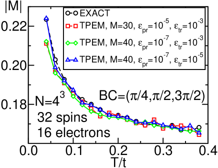
Figure 7: $|M|$ vs. $T/t$ on a $4^{3}$ lattice calculated using the TPEM with the parameters indicated. The result given by the diagonalization method is also shown. 10,000 thermalization Monte Carlo iterations and 10,000 measurements were performed. The same random configuration for the spatial location of the classical spins was considered in all cases.

The Hamiltonian for the diluted spin-fermion model that will be considered here is given by Eq. (11) except that the exchange term is replaced by $J\sum_{i\in I}\vec{S}_{i}\cdot\vec{\sigma}_{i}$, i. e. localized spins are present on only a subset $I$ of the lattice sites. Through nearest-neighbor hopping, the carriers can hop to any site of the square or cubic lattice. In the same way as in the case of the double-exchange model, for diluted systems we have used periodic boundary conditions for faster convergence. These are specified by the phases $(\pi/4,\pi/2,3\pi/4)$ in the $x$, $y$ and $z$ directions respectively.
It is important to remark that Monte Carlo calculations on diluted spin systems with concentration $x<1$ are $1/x$ times faster than the concentrated case since there are less sites with spins to propose a spin change.
In this case the density of states will have a more complicated shape, usually including a small impurity band. Therefore, it is interesting to see whether the TPEM is capable of treating this case. The comparison is provided in Fig. 7 for a concentration of 32 spins on a $4^{3}$ lattice with approximately 16 electrons, where it can be seen that the TPEM algorithm converges for $M=40$, $\epsilon_{tr}=10^{-7}$ and $\epsilon_{pr}=10^{-5}$. This simple test shows that even in the case of systems with impurity bands and positional disorder, the expansion yields results compatible with the exact treatment. Therefore, there is much potential for the use of this technique in the area of diluted magnetic semiconductors.

5.3 Convergence

The expansion parameters required for convergence, i. e. the cutoff $M$ and the thresholds $\epsilon_{tr}$ and $\epsilon_{pr}$, can be calculated on a small lattice where the exact diagonalization technique can be used to check the T/PEM algorithm. Since these numbers do not depend on the size of the system (only on the model, see re:furukawa03 ) then they can be safely used on larger lattices. This is shown in Fig. 7 where unlike for the concentrated system in this case neither $M=30$ nor $\epsilon_{tr}=10^{-5}$ is enough for convergence but $M=40$, $\epsilon_{tr}=10^{-7}$ and $\epsilon_{pr}=10^{-5}$ is required. On the other hand, the double-exchange model, Eq.(11), with infinite $J$ (not studied here but discussed in re:motome03 ) converges with a cutoff smaller than $M=30$. This is because the finite coupling system density-of-states is composed of two disconnected bands separated by approximately $2J$ and so the spectrum extends over a wide range of energies whereas in the infinite coupling system there is a single connected band resulting in a faster convergence.
Therefore, the reader and user of the TPEM library should not assume that the values presented in the previous examples will guarantee convergence for a particular model but should instead perform a check similar to the one presented in this section to determine the minimum value of the cutoff $M$ and the maximum values of $\epsilon_{tr}$ and $\epsilon_{pr}$ required for convergence.

6 Conclusions

In summary, we have provided a software library that implements the TPEM for fermion systems coupled to classical fields. This library will allow theorists to study a variety of systems employing the TPEM at the same level that, for instance, the LAPACK library laug is being used for exact diagonalization.
The TPEM has an enormous potential. For example, studies of diluted magnetic semiconductors that had not been possible before with more than one band will now be accessible and the results will be presented elsewhere. These studies are crucial to understand the properties of magnetic semiconductors and will help in the search for similar compounds with higher Curie temperatures. These high-Curie temperature compounds would in turn be useful for technological applications, for example in the fabrication of spin electronic or spintronic devices re:zutic04 . The possibility of studying larger systems will not merely imply a better estimation of the physical observables but will allow for the study of more complex systems like transition metal oxides with realistic bands and nanostructures.

7 Acknowledgments

This work was supported in part by NSF grants DMR-0122523, DMR-0312333, and DMR-0303348. G.A. performed this research as a staff member at the Oak Ridge National Laboratory, managed by UT-Battelle, LLC, for the U.S. Department of Energy under Contract DE-AC05-00OR22725. Most calculations were performed on the CMT computer cluster at the NHMFL and we acknowledge the help of T. Combs. J. Burgy helped with the design of the software library. We would like to thank also K. Foster for proofreading the manuscript.

8 Test Run Output

********************************************************
****** TESTING TRUNCATED POLYNOMIAL EXPANSION **********
********************************************************

This testing program calculates model properties in two ways:
(i)  Using standard diagonalization
(ii) Using the truncated polynomial expansion method
All tests are done for a nearest neighbor interaction with
random (diagonal) potentials.

-------------------------------------------------------------
TEST 1: MEAN VALUE FOR THE FUNCTION:
        N(x) =  0.5 * (1.0 - tanh (10.0 * x))

** Using diagonalization <N>=195.349187
** Using TPEM <N>=(cutoff--> infinity) lim<N_cutoff> where <N_cutoff> is
cutoffΨ<N_cutoff>Ψ%Error(compared to diag.)
10Ψ194.740524890737Ψ0.311577%
11Ψ194.921830592607Ψ0.218765%
12Ψ194.265186764692Ψ0.554904%
13Ψ194.136543222392Ψ0.620757%
14Ψ194.315979389497Ψ0.528903%
15Ψ194.408557066075Ψ0.481512%
16Ψ194.679187298809Ψ0.342975%
17Ψ194.612068307437Ψ0.377334%
18Ψ195.036519662839Ψ0.160056%
19Ψ195.085374546781Ψ0.135047%
20Ψ195.361097093739Ψ0.006097%
21Ψ195.325459995073Ψ0.012146%
22Ψ195.550660927328Ψ0.103135%
23Ψ195.576686770534Ψ0.116458%
24Ψ195.568643202933Ψ0.112340%
25Ψ195.549624351656Ψ0.102605%
26Ψ195.521318469307Ψ0.088115%
27Ψ195.535221730693Ψ0.095232%
28Ψ195.475638686769Ψ0.064731%
29Ψ195.465473123028Ψ0.059527%
30Ψ195.430165380516Ψ0.041453%
31Ψ195.437598886027Ψ0.045258%
32Ψ195.398432059641Ψ0.025209%
33Ψ195.392996060833Ψ0.022426%
34Ψ195.392858690195Ψ0.022356%
35Ψ195.396834086245Ψ0.024391%
36Ψ195.380978851635Ψ0.016274%
37Ψ195.378071566221Ψ0.014786%
38Ψ195.355235557817Ψ0.003096%
39Ψ195.357361742974Ψ0.004185%
40Ψ195.345473742639Ψ0.001901%
-------------------------------------------------------------
TEST 2: MEAN VALUE FOR THE FUNCTION:
        E(x) = 5.0 * x * (1.0 - tanh (10.0 * x))

** Using diagonalization <E>=-802.327051
** Using TPEM <E>=(cutoff--> infinity) lim<E_cutoff> where <E_cutoff> is
cutoffΨ<E_cutoff>Ψ%Error(compared to diag.)
(OUTPUT OMITTED, SEE FIG 2a)

-------------------------------------------------------------
TEST 3: MEAN VALUE AND DIFFERENCE FOR THE FUNCTION:
        S(x) =  log (1.0 + exp (-20.0 * x))

** Using diagonalization <S[matrix0]>= 854.249004021717
** Using diagonalization <S[matrix1]>= 846.624672679166
** Using diagonalization <S[matrix1]>-<S[matrix0]>=7.624331342551
** Using TPEM <S>=(cutoff--> infinity) lim<S_cutoff>
cutoffΨDelta_S_cutoffΨS_cutoff[diff]ΨError (to diag.)
(OUTPUT OMITTED, SEE FIG 2b)
-------------------------------------------------------------

References

- [1] Y. Motome, N. Furukawa, J. Phys. Soc. Japan 68 (1999) 3853.
- [2] N. Furukawa, Y. Motome, H. Nakata, Monte carlo algorithm for the double exchange model optimized for parallel computations, Computer Physics Communications 142 (2001) 410.
- [3] N. Furukawa, Y. Motome, Order N Monte Carlo algorithm for fermion systems coupled with fluctuating adiabatical fields, J. Phys. Soc. Jpn. 73 (2004) 1482.
- [4] E. Dagotto (Ed.), Nanoscale Phase Separation and Colossal Magnetoresistance, Springer Verlag, Berlin, 2002.
- [5] G. Alvarez, M. Mayr, E. Dagotto, Phase diagram of a model for diluted magnetic semiconductors beyond mean-field approximations, Phys. Rev. Lett. 89 (2002) 277202.
- [6] G. Alvarez, E. Dagotto, Journal of Magnetism and Magnetic Materials 272 (2002) 15.
- [7] G. Alvarez, E. Dagotto, Single-band model for diluted magnetic semiconductors: Dynamical and transport properties and relevance of clustered states, Phys. Rev. B. 68 (2003) 045202.
- [8] G. Alvarez, M. Mayr, A. Moreo, E. Dagotto, cond-mat/0401474, Predicting Colossal Effects in High Tc Superconductors (2004).
- [9] J. L. Alonso, L. A. Fernández, F. Guinea, V. Laliena, V. Martín-Mayo, Hybrid monte carlo algorithm for the double exchange model, Nucl. Phys. B 596 (2001) 587.
- [10] E. Dagotto, T. Hotta, A. Moreo, Colossal magnetoresistant materials: the key role of phase separation, Physics Reports 344 (2001) 1.
- [11] C. Zener, Interaction between the shells in the transition metals, Phys. Rev. 81 (1952) 440.
- [12] N. Furukawa, J. Phys. Soc. Japan 63 (1994) 3214.
- [13] F. F. Assaad, Phys. Rev. B 65 (2002) 115104.
- [14] H. Nakano, M. Imada, J. Phys. Soc. Jpn. 68 (1999) 1458.
- [15] Y. Motome, N. Furukawa, Critical temperature of ferromagnetic transition in three-dimensional double-exchange models, J. Phys. Soc. Japan 69 (2000) 3785, ERRATA: ibid., 70, 3186 (2001).
- [16] S. Yunoki, J. Hu, A. Malvezzi, A. Moreo, N. Furukawa, E. Dagotto, Phys. Rev. Lett. 80 (1998) 845.
- [17] A. Pelissetto, E. Vicari, Phys. Reports 368 (2002) 549.
- [18] Y. Motome, F. Furukawa, J. Phys. Soc. Jpn. 72 (2003) 2126.
- [19] E. Anderson, Z. Bai, C. Bischof, S. Blackford, J. Demmel, J. Dongarra, J. Du Croz, A. Greenbaum, S. Hammarling, A. McKenney, D. Sorensen, LAPACK Users’ Guide, 3rd Edition, Society for Industrial and Applied Mathematics, Philadelphia, PA, 1999.
- [20] I. Zutic, J. Fabian, S. D. Sarma, Spintronics: Fundamentals and applications, Rev. Mod. Phys. 76 (2004) 323.