Energy dependence of current noise in double-barrier normal-superconducting structures

Abstract

We study theoretically the current-noise energy dependence for a N-N’-S structure, where N and S stand for bulk normal metal and superconductor, respectively, and N’ for a short diffusive normal metal. Using quasiclassical theory of current fluctuations we obtain explicit expressions for the noise valid for arbitrary distributions of channel transparencies on both junctions. The differential Fano factor turns out to depend on both junction transparencies and the ratio of the two conductances. We conclude that measurement of differential conductance and noise can be used to probe the channel distribution of the interfaces.

Introduction

Current noise in hybrid mesoscopic systems has been deeply investigated in the last decade, both from the experimental and theoretical side.Blanter and Büttiker (2000); Nazarov (2002) It is quite clear now that noise contains piece of information on the charge transfer mechanism that is not present in the average current. The most striking example is clearly the carriers’ elementary charge, that can be obtained by measuring the noise-to-current ratio (Fano factor) in tunnel junctions. As a matter of fact, in mesoscopic Normal metal/Superconducting (N/S) hybrid structures, for energy (voltage bias and temperature) below the superconducting gap, the elementary process responsible for transport is Andreev reflection.Blonder et al. (1982); Beenakker (1997) It involves the transfer of two electrons at (nearly) the same time from the superconductor to the normal metal. This implies a doubling of the noise that has been predictedKhlus (1987); de Jong and Beenakker (1994) and observed.Jehl et al. (2000); Kozhevnikov et al. (2000) The situation is particularly clear in the tunneling limit, where the Fano-factor dependence on voltage and noise is exactly that for a normal metal with the replacement $e\rightarrow 2e$.Pistolesi et al. (2004) This behavior has been recently observed in semiconductor/Superconductor tunnel junctions.Lefloch et al. (2003)

N/S structures are also interesting for another reason. If the mesoscopic structure is shorter than the coherence length, transport is coherent and interference plays a crucial role. Since Andreev reflection involves scattering of an electron and a hole that are nearly time reversed particles, the random phases acquired during the diffusion in the metal are canceled out, and interference between electronic waves is controlled only by the length of the path and the energy of the particles.van Wees et al. (1992) This leads to a strong energy (temperature or voltage bias) dependence of the conductance that has been predictedVolkov et al. (1993); Hekking and Nazarov (1993, 1994) and measured.Kastalsky et al. (1991); Charlat et al. (1996) For large energies, phases acquire a fast dependence on position and transport becomes incoherent.

Very recently, the noise was also shown to have a non-trivial dependence on the energy. This dependence is different from that of the conductance.Belzig and Nazarov (2001a); Nazarov and Bagrets (2002) The cases of a long diffusive wire,Belzig and Nazarov (2001a); Houzet and Pistolesi (2004) tunnel junction,Stenberg and Heikkilä (2002); Pistolesi et al. (2004) and double tunnel barriersSamuelsson (2003) have been considered in the literature.

The last structure is particularly interesting since interference is enhanced by increasing the number of reflections. A Fabry-Perrot structure made of two barriers between the superconductor and the normal metal is expected to show a strong energy dependence conductance. This was predicted some time agoVolkov et al. (1993) for N-I-N’-I-S structures (where I is an insulating barrier) using quasiclassical Green’s function approach, and then confirmed experimentally.Quirion et al. (2002) More recently the noise in this tunneling structure has been calculated.Samuelsson (2003) The tunneling condition greatly simplifies the theoretical approach. This assumption does not limit severely the range of the normal-state conductances that can be theoretically investigated since the number of channels in most cases is very large. However, for given normal-state conductances one expects a dependence of current and noise on the actual value of the transparencies. Concerning the current, this was confirmed by the work of Clerk et al.Clerk et al. (2000) where the conductance for non-tunnel N-N’-S structures has been evaluated by means of random matrix theory. The behavior of the noise when the interfaces are not tunneling is the object of the present work.

In this paper we calculate the current noise for a N-N’-S structure without restrictions on the distribution of channel transparencies on both interfaces. We use quasiclassical Green’s function techniqueEilenberger (1968); Larkin and Ovchinninkov (1968); Usadel (1970) with boundary conditions modified by the introduction of a counting fieldLevitov et al. (1996); Nazarov (1999a); Belzig and Nazarov (2001b) allowing to calculate the noise. Exploiting the parametrization for the Green’s function proposed by two of the authors in Ref. Houzet and Pistolesi, 2004 we obtain the expressions for the voltage and temperature dependence of current noise in terms of a complex parameter to be found numerically. In some limiting cases the calculation can be performed to the end analytically. In all others the numerics is straightforward. We find that when the conductances are of the same order of magnitude, the channel distribution becomes crucial for the determination of the energy dependence of both the current and noise. The expressions we provide can be used to characterize interfaces when current and noise can be measured accurately. Even if this is non trivial from the experimental point of view, one should consider that it is very difficult to control only by means of the fabrication the transparency of an interface, i.e. the value of the transparencies and their distribution. If the average transparency can be easily estimated from the size of the contact, the true distribution remains out of the reach of any probe. That is why having a theory that predicts the conductance and noise for an arbitrary distribution of the channel transparencies can be a useful tool.

The paper is organized as follows. In Sec. I we introduce the circuit theory model and derive the main equations. In Sec. II we obtain the expressions for the current and the noise. We discuss our results for different distribution of channel transparencies. Sec. III gives our conclusions.

I Model and basic equations

We consider a N-N’-S structures with two junctions characterized by their set of channel transparencies: $\{\Gamma_{Nn}\}$ for the N-N’ barrier and $\{\Gamma_{Sn^{\prime}}\}$ for the N’-S barrier, $n$ and $n^{\prime}$ being channel labels (see Fig. 1). Consequently, the conductances are $g_{N(S)}=g_{Q}\sum_{n}\Gamma_{N(S)n}$, where $g_{Q}=2e^{2}/h$ is the quantum of conductance. We assume that $g_{N/S}$ is large enough to completely neglect the voltage drop in the N’ part. Namely, we require that the time necessary for an electron incoming from the leads to visit the whole N’ region (dwelling time $\tau_{D}$) is much smaller than the time spent in the region itself (escape time $\tau$). This corresponds to asking that the Thouless energy $E_{\textrm{Th}}\equiv\hbar/\tau_{D}=\hbar D/L^{2}$ ($D$ being the diffusive constant and $L$ the typical size of N’) is much larger than $E_{\tau}\equiv\hbar/\tau=(g_{N}+g_{S})\delta/(4\pi\,g_{Q})$ ($\delta$ being the average level spacing for N’). We also assume that $L\ll\xi_{d}=\sqrt{\hbar D/\Delta}$ (or equivalently $E_{\textrm{Th}}\gg\Delta$), where $\Delta$ is the superconducting gap of S, so that the spatial dependence of the proximity effect can be neglected in N’.

Proximity effect is thus completely controlled by $E_{\tau}$ and charge transport does not depend on the shape of N’. Hence we can consider N’ as an isotropic zero dimensional conductor.

Figure 1: Schematic picture of the N-N’-S junction. $\{\Gamma_{Nn}\}$ and $\{\Gamma_{Sn^{\prime}}\}$ are channel transparencies of the N-N’ and N’-S barriers.

We also assume that $g_{N/S}\gg g_{Q}$: Each barrier has a large number of conduction channels. Coulomb blockade and weak localization effects are then negligible. Finally we require that the escape time is much smaller than phase breaking and inelastic time. All these requirements are met, for instance, in the experiment of Ref. Quirion et al., 2002.

Within these assumptions, one can apply the so-called “circuit theory” to calculate current, noise and higher current cumulants.Nazarov (1999b, a); Belzig and Nazarov (2001b); Belzig (2002); Nazarov and Bagrets (2002) In particular the central region can be approximated with a single node, since any internal spatial dependence is negligible. The conductor is thus discretized into three nodes connected via two connectors, see Fig. 1. Each node is characterized by a quasiclassical matrix Green’s function in the Keldysh($\hat{\,}$)-Nambu($\bar{\,}$) space, $\check{G}_{N/S}$ for N and S leads and $\check{G}$ for N’ depending on the energy $E$ and a counting field $\chi$.Levitov et al. (1996)

The counting field appears as a modification of the boundary conditions. In our case this corresponds to transforming the normal reservoir Green’s function as follows:Belzig and Nazarov (2001b)

$$\check{G}_{N}(\chi)=e^{i\chi\check{\tau}_{K}/2}\ \check{G}_{N0}\ e^{-i\chi\check{\tau}_{K}/2},$$ (1)

where $\bar{\sigma}_{i},\hat{\tau}_{j(i,j=1,2,3)}$ are Pauli matrices, $\check{\tau}_{K}=\hat{\tau}_{3}\otimes\bar{\sigma}_{1}$, and $\check{G}_{N0}$ is the normal metal quasiclassical Green’s function in the diffusive limit (for a recent review see Ref. [Kopnin, 2001]):

$$\check{G}_{N0}=\left(\begin{array}[]{cc}\hat{\tau}_{3}&2(f_{T0}+f_{L0}\hat{\tau}_{3})\\ 0&-\hat{\tau}_{3}\end{array}\right).$$ (2)

Here, $f_{T0}=f(E-eV)-f(E+eV)$, $f_{L0}=1-f(E+eV)-f(E-eV)$, $f$ is the Fermi function at temperature $T$, and $V$ is the voltage bias between the normal metal and the superconducting reservoir.

The Green’s function in the superconducting reservoir is

$$\check{G}_{S}=\left(\begin{array}[]{cc}\hat{R}_{S}&\hat{K}_{S}\\ 0&\hat{A}_{S}\end{array}\right).$$ (3)

Here, $\hat{R}_{S}$ is the retarded part given by:

$$\hat{R}_{S}=\frac{1}{\sqrt{(E+i\eta)^{2}-|\Delta}|^{2}}\left(\begin{array}[]{cc}E&\Delta\\ -\Delta^{\star}&-E\end{array}\right)$$ (4)

with the branch cut of the square root going from $-\Delta$ to $+\Delta$ on the real $E$ axis. The advanced part is given by $\hat{A}_{S}=-\hat{\sigma}_{3}\hat{R}^{{\dagger}}_{S}\hat{\sigma}_{3}$, and the Keldysh part follows by the equilibrium condition of the reservoir: $\hat{K}_{S}=(f(E)-f(-E))(\hat{A}_{S}-\hat{R}_{S})$. In the following, we focus on the supgap regime, so we can limit ourselves to $E\ll|\Delta|$. Moreover, since there is only one superconductor in the problem, we can choose $\Delta$ real. Then the matrix Green’s function of the superconductor simplifies to $\check{G}_{S}=\hat{\tau}_{2}\otimes\bar{1}$.

The Green’s function in the central node satisfies the normalization condition $\check{G}^{2}=\check{1}$ and the symmetry property:Houzet and Pistolesi (2004); foo

$$\check{G}^{{\dagger}}(-\chi)=-\check{\tau}_{L}\ \check{G}(\chi)\ \check{\tau}_{L}$$ (5)

with $\check{\tau}_{L}=\hat{\tau}_{3}\otimes\bar{\sigma}_{2}$. (Similar relations hold for $\check{G}_{N/S}$ as well.) It is solution of the Usadel equation:Usadel (1970); Kopnin (2001)

$$\hbar D\mathbf{\mbox{\boldmath$\nabla$}}\left(\check{G}\mathbf{\mbox{\boldmath$\nabla$}}\check{G}\right)-iE[\check{G}_{E},\check{G}]=0\,,\qquad\check{G}_{E}=\hat{\tau}_{3}\otimes\bar{1}\,.$$ (6)

We integrate this equation over the volume $\mathcal{V}$ of N’. Using the divergence theorem, it gives:

$$\int_{\partial\mathcal{V}}d^{2}\mathbf{S}\cdot\left(\sigma_{0}\check{G}\mathbf{\mbox{\boldmath$\nabla$}}\check{G}\right)-2\,i\frac{e^{2}\nu_{0}\mathcal{V}\,E}{\hbar}\,[\check{G}_{E},\check{G}]=0\,,$$ (7)

where $\nu_{0}$ is the density of states per spin of N’, and $\sigma_{0}=2e^{2}D\nu_{0}$ its conductivity in the normal metallic state. Using boundary conditions for the Green’s functions over the surface $\partial V$ of the grain,Zaitsev (1984); Nazarov (1999b) we have:

$$-\int_{\partial\mathcal{V}}d^{2}\mathbf{S}.\left(\sigma_{0}\check{G}\mathbf{\mbox{\boldmath$\nabla$}}\check{G}\right)=\check{I}_{N}+\check{I}_{S}$$ (8)

with

$$\check{I}_{N} = g_{Q}\sum_{n}\frac{2\,\Gamma_{Nn}[\check{G}_{N}(\chi),\check{G}(\chi)]}{4+\Gamma_{Nn}(\{\check{G}_{N}(\chi),\check{G}(\chi)\}-2)},$$ (9a)

$$\check{I}_{S} = g_{Q}\sum_{n}\frac{2\,\Gamma_{Sn}[\check{G}_{S},\check{G}(\chi)]}{4+\Gamma_{Sn}(\{\check{G}_{S},\check{G}(\chi)\}-2)}\,.$$ (9b)

Then $\check{G}$ is fully determined by Eq. (6) which takes the form of a conservation-like equation for the spectral matrix current:

$$\check{I}_{N}+\check{I}_{S}+\check{I}_{E}=0\,,$$ (10)

where

$$\check{I}_{E} = g_{Q}\frac{2i\pi\,E}{\delta}[\check{G}_{E},\check{G}(\chi)]\,.$$ (11)

Here $\check{I}_{E}$ is the “leakage” matrix current,Nazarov (1999b) which takes into account the relative dephasing between electron and hole during their propagation in the central node N’, whose mean level spacing is $\delta=1/(\nu_{0}V)$. The estimate for the inverse escape time, $E_{\tau}/\hbar=\delta(g_{N}+g_{S})/(4\pi\hbar\,g_{Q})$, follows from comparison between the amplitudes of $\check{I}_{N}+\check{I}_{S}$ and $\check{I}_{E}$.

Once the matrix $\check{G}(\chi)$ is known, current, zero frequency noise and all higher current cumulants can be obtained by differentiation of $I(\chi)$ defined as follows:

$$I(\chi)=-\frac{1}{8e}\int\mathrm{d}E\ \textrm{tr}[\check{\tau}_{K}\check{I}_{N}]\,.$$ (12)

(By matrix current conservation (10) $I(\chi)$ equals minus expression (12) with $\check{I}_{N}$ substituted by $\check{I}_{S}$.) The first two moments are the average current,

$$I=I(\chi)\big{|}_{\chi=0}\,,$$ (13)

and the current noise,

$$S=2ie\left.\frac{\partial I(\chi)}{\partial\chi}\right|_{\chi=0}\,.$$ (14)

For tunneling interfaces, $\Gamma_{n}\ll 1$, the boundary conditions simplifies since one can neglect the anticommutator in the denominator of Eqs. (9a) and (9b). In that limit the matrix $\check{G}(\chi)$ can be found analytically.Börlin et al. (2002); Samuelsson (2003) It is thus possible to study not only the current and noise, but the whole set of cumulants. In the general case of arbitrary value of $\Gamma_{n}$ there is no analytical solution available for $\check{G}(\chi)$.

If one restricts to the first two cumulants, $I$ and $S$, which are more accessible experimentally, it is possible to write simplified equations for the coefficient of the expansion of $\check{G}$ in $\chi$:Belzig and Nazarov (2001a); Houzet and Pistolesi (2004)

$$\check{G}(\chi)=\check{G}_{0}-i\frac{\chi}{2}\check{G}_{1}+\mathcal{O}(\chi^{2})\,.$$ (15)

Finding $\check{G}_{0}$ gives the current while $\check{G}_{1}$ leads to the noise. In the following we follow this program and solve (10) for the first two orders in $\chi$.

II Current and Noise

II.1 Current evaluation

To obtain the current one has to evaluate Eq. (12). For this, we need $\check{G}_{0}$ as defined in Eq. (15). A crucial step to solve the problem is to take into account the normalization condition without redundancy in the parametrization. When the counting field vanishes, the solution is well known and it consists in the following parametrization of $\check{G}_{0}$:

$$\check{G}_{0}=\left(\begin{array}[]{cc}\hat{R}&\hat{K}\\ 0&\hat{A}\end{array}\right)$$ (16)

with

$$\hat{R} = \hat{\tau}_{3}\cosh\theta+i\hat{\tau}_{2}\sinh\theta\,,\quad\hat{A}=-\hat{\tau}_{3}\ \hat{R}^{{\dagger}}\ \hat{\tau}_{3}\,,$$ (17a)

$$\hat{K} = \hat{R}\hat{f}-\hat{f}\hat{A},\qquad\hat{f}=f_{L}+\hat{\tau}_{3}f_{T}\,.$$ (17b)

Here, the parameters $f_{T}$ and $f_{L}$ are real, as follows from Eq. (5) at $\chi=0$. The complex number $\theta$ characterizes the paring in the grain: $\theta=-i\pi/2$ corresponds to a fully superconducting state and $\theta=0$ to a normal one. Substituting this form for $\check{G}_{0}$ into Eq. (10) at $\chi=0$ one can determine $\theta$, $f_{L}$, and $f_{T}$. The retarded or advanced parts give the equation for $\theta$:

$$g_{N}\langle Z_{N}\rangle\sinh\theta+i\varepsilon g_{D}\sinh\theta+ig_{S}\langle Z_{S}\rangle\cosh\theta=0,$$ (18)

where $\varepsilon=E/E_{\tau}$, $g_{D}=g_{N}+g_{S}$, $Z_{N}=[1+\Gamma_{N}(\cosh\theta-1)/2]^{-1}$ and $Z_{S}=[1+\Gamma_{S}(i\sinh\theta-1)/2]^{-1}$. Here,

$$\langle f(\Gamma_{\alpha})\rangle={\sum_{n}\Gamma_{\alpha n}f(\Gamma_{\alpha n})\over\sum_{n}\Gamma_{\alpha n}}\,$$ (19)

stands for the average over channel transparencies with $\alpha=$ N or S. The Keldysh part of the spectral-current-conservation equation (10) gives $f_{L}=f_{L0}$ and $f_{T}/f_{T0}=c$ with

$$c=\frac{g_{N}\tanh\theta_{1}}{2\,\varepsilon g_{D}\sin\theta_{2}}\langle\left[(2-\Gamma_{N})\,\cos\theta_{2}+\Gamma_{N}\,\cosh\theta_{1}\right]|Z_{N}|^{2}\rangle.$$

Here, we used the decomposition $\theta=\theta_{1}+i\theta_{2}$ into real and imaginary part. Finally, the mean current is given by

$$I=\frac{1}{2e}\int^{\infty}_{-\infty}\mathrm{d}E\,f_{T0}\,\mathcal{G}(E)$$ (21)

with

$$\mathcal{G}(E) = c\,g_{S}\,\cosh\theta_{1}$$

$$\times\,\langle\large[-\sin\theta_{2}+\Gamma_{S}\,(\cosh\theta_{1}\,+\,\sin\theta_{2})/2\large])|Z_{S}|^{2}\rangle\,.$$

At zero temperature the differential conductance $G\equiv\mathrm{d}I/\mathrm{d}V$ equals $\mathcal{G}(eV)$. For uniform transparency, expression (II.1) coincides with that obtained by Clerk et al. in Ref. Clerk et al., 2000 using random matrix theory.

We now discuss the conductance for small and large energy. Let us begin with the low energy limit $eV\ll E_{\tau}$, i.e., the completely coherent case. $\theta$ is then an imaginary number. Eq. (II.1) reduces to:

$$G^{-1}_{\textrm{coh}}=(\widetilde{g}_{N})^{-1}+(\widetilde{g}_{S})^{-1}\,,$$ (23)

where

$$\widetilde{g}_{N} = g_{N}\cos\alpha\langle\widetilde{Z}^{2}_{N}\rangle+g_{N}\langle\Gamma_{N}\widetilde{Z}^{2}_{N}\rangle(1-\cos\alpha)/2\,,$$

$$\widetilde{g}_{S} = g_{S}\sin\alpha\langle\widetilde{Z}^{2}_{S}\rangle+g_{S}\langle\Gamma_{S}\widetilde{Z}^{2}_{S}\rangle(1-\sin\alpha)/2\,,$$

with $\widetilde{Z}_{N}=[1+\Gamma_{N}(\cos\alpha-1)/2]^{-1}$ and $\widetilde{Z}_{S}=[1+\Gamma_{S}(\sin\alpha-1)/2]^{-1}$. The real parameter $\alpha=-\textrm{Im}(\theta)$ is the solution of the equation:

$$g_{N}\,\sin\alpha\,\langle\widetilde{Z}_{N}\rangle=g_{S}\,\cos\alpha\,\langle\widetilde{Z}_{S}\rangle\,.$$ (24)

Coherent conductance strongly depends on the ratio $g_{N}/g_{S}$. When the central island is well connected to N ($g_{N}\gg g_{S}$) $\theta=0$. The grain is in the normal state. Then differential conductance is given by $G_{\textrm{coh}}=g^{\textrm{And}}_{S}=2g_{S}\langle\Gamma_{S}/(2-\Gamma_{S})^{2}\rangle$: the charge transfer is dominated by Andreev reflection at N’-S interface.Beenakker (1992) In the opposite case of an island well connected to S ($g_{N}\ll g_{S}$) $\theta=-i\pi/2$, the grain is superconducting and we have $G_{\textrm{coh}}=g^{\textrm{And}}_{N}=2g_{N}\langle\Gamma_{N}/(2-\Gamma_{N})^{2}\rangle$. This means that conductance is dominated by Andreev reflection at N-N’ barrier. We can also note that $G_{\textrm{coh}}$ is invariant under the transformation $\{\Gamma_{Nn}\}\leftrightarrow\{\Gamma_{Sn^{\prime}}\}$ in Eq. (23). Thus when an electron crosses the N-N’-S structure, it can not distinguish which barrier is closer to the superconductor.

In the opposite limit of $eV\gg E_{\tau}$ transport is incoherent. The large energy mismatch between electrons and Andreev reflected holes washes out interference effects. We find the following expression for the conductance

$$G_{\textrm{class}}^{-1}=g_{N}^{-1}+(g^{\textrm{And}}_{S})^{-1}\,,$$ (25)

that is now no more invariant for exchange of the N-S and N’-S barriers. The grain is in the normal state ($\theta=0$). The physical interpretation for the incoherent transport is simple since one can treat one channel at the time (electrons do not interfere). For a Cooper pair to be transferred across the double barrier structure the electron has to undergo the following steps: crossing of the N-N’ barrier, Andreev conversion to a hole at the N’-S junction (with probability $R_{Sn^{\prime}}=\Gamma^{2}_{Sn^{\prime}}/(2-\Gamma_{Sn^{\prime}})^{2}$ per channel), and finally crossing of the N-N’ barrier (see Fig. 2).

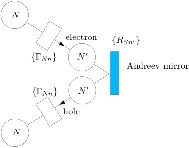
Figure 2: Schematic picture of the N-N’-S junction in the incoherent regime. Electrons are Andreev reflected into hole at N’-S barrier.

Thus in the incoherent limit, the double junction is equivalent to three junctions in series of transparencies $\{\Gamma_{Nn}\}$, $\{R_{Sn^{\prime}}\}$ and $\{\Gamma_{Nn}\}$, respectively, with an elementary transferred charge $2e$. Conductance is then given by Ohm’s law for the three conductances in series multiplied by a factor two: $G_{\textrm{class}}=2[(g_{Q}\sum_{n}\Gamma_{Nn})^{-1}+(g_{Q}\sum_{n^{\prime}}R_{Sn^{\prime}})^{-1}+(g_{Q}\sum_{n}\Gamma_{Nn})^{-1}]^{-1}$, which coincides with Eq. (25).

Figure 3: Differential conductance normalized by its classical value as a function of $eV/E_{\tau}$ for two disordered interfaces at zero temperature. A peak appears near $eV\approx E_{\tau}$ when $g_{N}\approx g_{S}$ and it becomes sharper for $g_{N}/g_{S}\rightarrow 0$.

For intermediate energies, the shape of $G$ depends both on the ratio of the two conductances and the set of channel transparencies. A particularly relevant case of channel distribution is that of a disordered interface:Schep and Bauer (1997)

$$\rho_{\alpha}(\Gamma)\equiv\sum_{n}\delta(\Gamma-\Gamma_{\alpha n})=\frac{g_{\alpha}}{g_{Q}\,\pi}\frac{1}{\Gamma^{3/2}\sqrt{1-\Gamma}}\,,$$ (26)

where $\alpha=$N or S. We plot the conductance for this case and different values of the ration $g_{S}/g_{N}$ in Fig. 3. Qualitatively one sees a cross-over from a “reflectionless” tunneling behavior, typical of tunnel junctions (with a zero-bias peak) to a “re-entrant” behavior with a peak at $eV$ of the order of $E_{\tau}$. In both cases the qualitative explanation is simple. In the tunnel case, the electron tries many times to enter the superconductor. At low energy, the corresponding quantum paths add coherently, giving a large resulting current. Any increase in the energy reduces the coherent contribution to the current since interference is suppressed and, thus, the mixed terms vanish. This explains the zero-bias peak in the $G(V)$ plot. On the other hand, when the superconducting barrier is transparent the electrons always succeed in being converted to holes, but Andreev reflection comes with a phase factor ($-i$) that induces destructive interference among electronic waves for $E=0$.Beenakker (2000) The loss of coherence among waves can thus enhance the current leading to a maximum in the $G(V)$ plot. This behavior is very similar to the one observed in a diffusive wire.Volkov et al. (1993) One sees nevertheless that the effect is much larger here, since the Fabry-Perot structure enhances interference. We will discuss the role of barrier transparencies in II.3.

II.2 Noise evaluation

Let us now consider the main subject of the paper: the noise. As stated above we need to solve Eq. (10) in first order in $\chi$. We expand thus each spectral current: $\check{I}_{\beta}=\check{I}^{0}_{\beta}+\chi\check{I}^{1}_{\beta}+\mathcal{O}(\chi^{2})$ with $\beta=$N, S, or E. We obtain:

$$\check{I}^{1}_{N} = ig_{N}\big{(}\langle\check{D}_{N}\rangle([\check{G}_{N1},\check{G}_{0}]-[\check{G}_{N0},\check{G}_{1}])$$

$$-\langle\Gamma_{N}[\check{G}_{N0},\check{G}_{0}]\check{D}_{N}(\{\check{G}_{N1},\check{G}_{0}\}-\{\check{G}_{N0},\check{G}_{1}\})\check{D}_{N}\rangle\big{)}\,,$$

$$\check{I}^{1}_{S} = -ig_{S}\big{(}\langle\check{D}_{S}\rangle[\check{G}_{S},\check{G}_{1}]$$

$$-\langle\Gamma_{S}[\check{G}_{S},\check{G}_{0}]\check{D}_{S}\{\check{G}_{S},\check{G}_{1}\}\check{D}_{S}\rangle\big{)}\,,$$

$$\check{I}^{1}_{E} = \frac{g_{D}\varepsilon}{4}[\check{G}_{E},\check{G}_{1}]\,,$$

with $\check{D}_{\alpha}=(4+\Gamma_{\alpha}(\{\check{G}_{\alpha 0},\check{G}_{0}\}-2))^{-1}$, $\alpha=$N or S, and $\check{G}_{N1}=[\check{\tau}_{K},\check{G}_{N0}]$. Zero frequency current noise is given by

$$S=\frac{i}{4}\int\mathrm{d}E\ \textrm{tr}[\check{\tau}_{K}\check{I}^{1}_{S}]\,.$$ (27)

Here, the unknown matrix $\check{G}_{1}$, cf. Eq. (15), satisfies

$$\check{I}^{1}_{N}+\check{I}^{1}_{S}+\check{I}^{1}_{E}=0\,.$$ (28)

Additionally the normalization of $\check{G}$ implies $\{\check{G}_{0},\check{G}_{1}\}=0$. This can be satisfied by defining $\check{G}_{1}=[\check{G}_{0},\check{\phi}]$ for any $\check{\phi}$. We use the parametrization found in Ref. Houzet and Pistolesi, 2004 for the matrix $\check{\phi}$:

$$\check{\phi}=\left(\begin{array}[]{cc}af_{T0}\hat{\tau}_{1}-c\hat{f}\hat{\tau}_{3}&b\hat{\tau}_{3}+d\\ c\hat{\tau}_{3}&a^{\ast}f_{T0}\hat{\tau}_{1}+c\hat{f}\hat{\tau}_{3}\end{array}\right)\,.$$ (29)

The symmetry condition (5) on $\check{G}$ implies that $\check{\phi}^{{\dagger}}=-\check{\tau}_{L}\check{\phi}\check{\tau}_{L}$; it follows that $b$, $c$, and $d$ are real, while $a$ is complex. The parameter $c$ has been already given in Eq. (II.1). Inserting this form for $\check{\phi}$ into Eq. (28) one obtains a complete set of equations for all the parameters of $\check{\phi}$. The equation for $a$ is given by the antidiagonal elements of the retarded part of Eq. (28). The Keldysh part of the same equation gives the equations for $b$ and $d$. Finally, using Eq. (27), zero frequency current noise takes the form:

$$S=\int\mathrm{d}E\,\,\{\mathcal{G}(E)[1-f^{2}_{L0}]+\mathcal{S}_{T}(E)\,f^{2}_{T0}\}\,.$$ (30)

The rather cumbersome expressions for $a$, $b$, $d$, and $\mathcal{S}_{T}$ are given in the Appendix. Here we only stress that the analytic expressions for the coefficients all depend on a single complex number, $\theta$, solution of Eq. (18). Even if $\theta$ is given by the solution of an algebraic equation it is not always possible to obtain an analytical expression for it. Nevertheless, once this parameter is known numerically, it is enough to substitute it into the expressions given in the Appendix to obtain the value of the current noise. Note that knowledge of $\theta$ is already necessary to obtain the conductance.

Let us now discuss the result in some details. We first note that Eq. (30) for $eV\ll k_{B}T$ correctly agrees with the fluctuation-dissipation theorem.Callen and Welton (1951) As a matter of fact, in this case $f_{T}=0$ and the remainder gives precisely $S=4k_{B}T\,G(T)$. In the opposite limit noise is not simply related to the conductance and has to be computed with Eq. (30). In the zero temperature limit ($k_{B}T\ll eV$, $E_{\tau}$) the experimentally accessible differential Fano factor becomes from Eq. (30):

$$F(V)\equiv\frac{1}{2eG(V)}\,\frac{\mathrm{d}S(V)}{\mathrm{d}V}=1+\frac{\mathcal{S}_{T}(eV)}{\mathcal{G}(eV)}\,.$$ (31)

Let us now discuss as in the conductance case the two analytically tractable limits: the completely coherent and incoherent cases. In the coherent limit one can obtain closed analytical expression for the noise depending on the parameter $\alpha$ solution of Eq. (24). However they are rather cumbersome and we will not show them. In the specific case of two transparent barriers, we recover the recent analytical result of Vanević et al. in Ref. [van, ]. Similarly to the conductance, the expression for the Fano factor is left unchanged when the set of transparencies of the two barriers are exchanged: $\{\Gamma_{Nn}\}\leftrightarrow\{\Gamma_{Sn^{\prime}}\}$. The Fano factor depends on the ratio $g_{N}/g_{S}$. If the grain is well connected to the superconductor ($g_{N}\ll g_{S}$), $F_{\textrm{coh}}=2\sum_{n^{\prime}}R_{Sn^{\prime}}(1-R_{Sn^{\prime}})/\sum_{n^{\prime}}R_{Sn^{\prime}}$: we obtain the Fano factor of N’-S interface alone.de Jong and Beenakker (1994) In the opposite limit, $g_{N}\gg g_{S}$, $F_{\textrm{coh}}=2\sum_{n}R_{Nn}(1-R_{Nn})/\sum_{n}R_{Nn}$: the Andreev reflection occurs at N’-N barrier. It is interesting to notice that even if transport properties ($G_{\textrm{coh}}$ and $F_{\textrm{coh}}$) do not depend on the relative position of the barriers, the state of the grain does. It can be normal or fully superconducting depending on $g_{N}/g_{S}$.

We consider now the incoherent limit: $eV\gg E_{\tau}$. From Eq. (31) we find the following explicit form for the differential Fano factor

$$F_{\textrm{class}} = \biggl{[}(g^{\textrm{And}}_{S})^{3}\frac{\sum_{n}\Gamma_{Nn}\,(1-\Gamma_{Nn}/2)}{{\sum_{n}\Gamma_{Nn}}}+2g_{N}g^{\textrm{And}}_{S}(g_{N}+g^{\textrm{And}}_{S})+2g^{3}_{N}\frac{\sum_{n}R_{Sn}\,(1-R_{Sn})}{{\sum_{n}R_{Sn}}}\biggr{]}\frac{1}{(g_{N}+g^{\textrm{And}}_{S})^{3}}.$$ (32)

This result can also be found using the technique developed by Belzig and Samuelsson.Belzig and Samuelsson (2003) The physical interpretation is the same described for $G_{\textrm{class}}$, the only difference is that here we need to calculate the current fluctuation at each barrier instead of the current. Indeed, in the classical limit, the structures can be schematized as a series of three junctions of transparencies $\{\Gamma_{Nn}\}$, $\{R_{Sn^{\prime}}\}$, and $\{\Gamma_{Nn}\}$ with decoherent cavities in between. Again the elementary transferred charge is $2e$ (see Fig.2). The Fano factor for a series of two junctions separated by a decoherent cavity has been evaluated (for elementary charge $e$):Nazarov and Bagrets (2002); Nagaev et al. (2002)

$$F_{12}(g_{1},F_{1};g_{2},F_{2})=\frac{g^{3}_{1}F_{2}+g_{1}g_{2}(g_{1}+g_{2})+g^{3}_{2}F_{1}}{(g_{1}+g_{2})^{3}}\,,$$ (33)

where $g_{i}=g_{Q}\sum_{n}\Gamma_{in}$ and $F_{i}=(\sum_{n}\Gamma_{in}(1-\Gamma_{in}))/\sum_{n}\Gamma_{in}$, $i=$ 1 or 2. From Eq. (33) the Fano factor for three junctions in series can be easily obtained: $F_{123}(g_{1},F_{1};g_{2},F_{2};g_{3},F_{2})=F_{12}(g_{12},F_{12};g_{3},F_{3})$ with $g_{12}=g_{1}g_{1}/(g_{1}+g_{2})$. This expression coincides with Eq. (32), once we take into account the doubling of the charge. Let us now consider the case when one of the two interfaces dominates transport. For $g^{\textrm{And}}_{S}\ll g_{N}$, N’-S junctions controls charge transfer and it is thus not surprising to find that the Fano factor is that of the N-S barrier alone:de Jong and Beenakker (1994) $F_{\textrm{class}}=2\,\sum_{n}R_{Sn}\,(1-R_{Sn})/{\sum_{n}R_{Sn}}$. In the opposite limit of $g^{\textrm{And}}_{S}\gg g_{N}$, we have instead the following result: $F_{\textrm{class}}=\sum_{n}\Gamma_{Nn}\,(1-\Gamma_{Nn}/2)/{\sum_{n}\Gamma_{Nn}}$. Note that it differs from the Fano factor for a single interface of transparency distribution $\Gamma_{Nn}$. Actually even if the resistance is dominated by the N’-N interface, the presence of the N-S interface doubles the number of interfaces, leading to this result. Note also that for a completely transparent N’-N interface we have a finite noise $F=1/2$. The conductance in this limit is $g_{N}$ [cf. Eq. (25)]. Again one could expect that $F$ should be zero, but actually transport is slightly more subtle. The effective system is that of a chaotic cavity connected through two completely transparent interfaces of conductance $g_{N}$ to the two leads. The electron entering the cavity from the normal side has probability 1/2 of exiting from the same interface as an electron and 1/2 of exiting as a hole on the other side. In the second case the transferred charge is $2e$ with probability 1/2. Thus the effective conductance is $g_{N}$, like for a normal Sharvin contact, but with an effective Fano factor of 2 (for the charge) times 1/4 (for the $\Gamma(1-\Gamma)$ term).

Figure 4: Differential Fano factor as a function of $eV/E_{\tau}$ for two disordered interfaces at zero temperature. A dip appears for $eV\approx E_{\tau}$ when $g_{N}\approx g_{S}$ and increases for $g_{N}/g_{S}$ decrease.

For intermediate values of the energy, noise, like the conductance, has to be considered numerically. Our results allow to study any situation. We plot in Fig. 4 the Fano factors for the same parameters considered for the conductance in Fig. 3. The qualitative behavior resembles that of the noise in long diffusive structures. In particular a minimum at finite voltage for the Fano factor is present when $g_{S}\gg g_{N}$. This is very similar to the minimum in the differential Fano factor for a wire in good contact with normal and superconducting reservoirs.Belzig (2002); Kozhevnikov et al. (2000)

II.3 Effect of the channel distribution on current and noise

Figure 5: Differential conductance and Fano factor as a function of $eV/E_{\tau}$ at zero temperature. Channel transparencies of the two interfaces have unimodal distribution. In the left panel, N’-S junction is tunnel ($\Gamma_{S}=0.01$) and in the right panel N’-S junction is transparent ($\Gamma_{S}=1$).

Figure 6: Differential conductance and Fano factor as a function of $eV/E_{\tau}$ at zero temperature. Channel transparencies of the two interfaces have unimodal distribution. In the left panel, N-N’ junction is tunnel ($\Gamma_{N}=0.01$) and in the right panel N-N’ junction is transparent ($\Gamma_{N}=1$).

Let us now consider the genuine effect of the modification of the channel distribution. The optimal situation is when the normal-state conductances of the two interfaces are equal, so that the dependence on the distribution of the channel transparencies of both interface should be maximum. For simplicity in the presentation we will discuss only the case of $\Gamma_{n}=\Gamma$ for all $n$. We thus vary the transparency and the number of channels at each interface in such a way that the ratio of the normal-state conductance is kept equal to 1. Note when the channels are transparent this does not mean necessary that the contact region must be very small (to keep the same conductance of the tunneling case). It is enough that the distribution of channels of a large junction is bimodal, with a large majority of the channels completely opaque ($\Gamma=0$) and few of them of the given transparency.

We calculated the energy dependence of the conductance and of the noise as a function of the transparency of the interfaces. Results are reported in Fig. 5 and Fig. 6. In Fig. 5 we set $\Gamma_{S}=0.01$ (left pannels) and $\Gamma_{S}=1$ (right pannels) and we vary $\Gamma_{N}$ from 0.1 to 0.9. In Fig. 5 we plot the same curves exchanging the role of $\Gamma_{N}$ and $\Gamma_{S}$.

First we note how important is the channel transparency to predict the value of both the conductance and the noise. Knowledge of the conductance alone is not enough. Once the conductance is known, the energy dependence of both current and noise can give valuable indications on the channel distribution. A second important remark is the qualitatively similar behavior of the conductance and the Fano factor. This is particularly evident for the case when $\Gamma_{N}\gg\Gamma_{S}$ (left panel of Fig. 5). The differential Fano factor is linearly related to the conductance, $F(E)\approx\gamma_{0}-\gamma_{1}G(E)$, with $\gamma_{0}$ and $\gamma_{1}$ positive constants. This behavior was proved analytically for tunneling contacts between a superconductor and a wire in Ref. Houzet and Pistolesi, 2004. Actually this behavior seems to be a general property of the whole set of plots, with variable accuracy. The differential Fano factor looks like the differential conductance upside down. This is only a qualitative behavior, the proportionality factor depends on the actual transparency, as was found in Ref. Houzet and Pistolesi, 2004.

III Conclusions

We studied the energy dependence of the current noise in a double barrier N-N’-S structure for arbitrary transparency of the barriers. In particular, we could describe the crossover between the completely coherent and incoherent regimes. The noise in the double-barrier structure ressembles the one found earlier in an extended geometry, like a wire. Namely, we found that the energy dependence of the current and noise are qualitatively strongly related though quantitatively independent. The distribution of transparencies at the barriers strongly influences both the current and noise. We suggest that a measurement of both quantities in the same sample would provide valuable information on the properties of the interfaces.

Appendix A Fano factor equations

In this appendix we give the explicit expressions for ${\cal S}$ and the coefficients $a$, $b$, and $d$, entering the definition of $\check{\phi}$. We use the shorthand notation $\cosh\theta_{1}={\tilde{c}}_{1}$ , $\sinh\theta_{1}={\tilde{s}}_{1}$, $\cos\theta_{2}=c_{2}$, and $\sin\theta_{2}=s_{2}$.

We begin with the three coefficients:

$$a=\frac{g_{N}\,\langle A_{0}\rangle+{\tilde{c}}_{1}\left(-2\,g_{N}\,c\,\langle A_{1}\rangle+c^{2}(g_{N}\,\langle A_{1}\rangle+g_{S}\,\langle A_{2}\rangle+2\,i\,g_{D}\,\varepsilon\,s_{2})\right)}{\langle B\rangle}$$ (34)

with

$$A_{0} = i\sinh\theta\,s_{2}^{2}\,\overline{Z_{N}}\,{Z_{N}}^{2}{\Gamma_{N}}^{2}+\Big{(}\big{(}2\,i\sinh\theta\,{\tilde{c}}_{1}c_{2}-i{\tilde{c}}_{1}{\tilde{s}}_{1}+c_{2}s_{2}\big{)}{Z_{N}}^{2}-2\,s_{2}c_{2}\overline{Z_{N}}Z_{N}\Big{)}\Gamma_{N}-2i\sinh\theta\,Z_{N}\,,$$

$$A_{1} = i\,\sinh\theta\,{\tilde{c}}_{1}s_{2}\overline{Z_{N}}\,{Z_{N}}^{2}{\Gamma_{N}}^{2}+\left(i\,\sinh\theta\,c_{2}{Z_{N}}^{2}-2\,{\tilde{c}}_{1}c_{2}s_{2}\overline{Z_{N}}\,Z_{N}\right)\Gamma_{N}+2\,Z_{N}\,s_{2}\,,$$

$$A_{2} = -\cosh\theta\,c_{2}^{2}\,{\tilde{c}}_{1}\overline{Z_{S}}\,{Z_{S}}^{2}{\Gamma_{S}}^{2}+\left(\cosh\theta\,{\tilde{c}}_{2}\,{Z_{S}}^{2}+2\,{\tilde{c}}_{1}s_{2}c_{2}\overline{Z_{S}}\,Z_{S}\right)\Gamma_{S}+2\,Z_{S}\,c_{2}\,,$$

$$B = ig_{S}\,{Z_{S}}{\Gamma_{S}}^{2}\cosh^{2}\theta-ig_{N}{Z_{N}}^{2}\,{\Gamma_{N}}\sinh^{2}\theta-2\,g_{S}\,\,Z_{S}\,\sinh\theta-2\,g_{D}\,\varepsilon\,\cosh\theta+2\,ig_{N}\,Z_{N}\,\cosh\theta\,.$$

Then

$$b = c\,(1-2f^{2}_{L0})+f^{2}_{T0}b_{T}$$ (36)

with

$$b_{T}=-2c^{3}+\frac{g_{N}}{4\varepsilon g_{D}}\left[\langle\beta_{0}\rangle c^{2}\frac{{\tilde{s}}_{1}}{s_{2}}-2c\,\left(\langle\beta_{0}\rangle\frac{{\tilde{s}}_{1}}{s_{2}}+\frac{a_{2}}{\tan\theta_{2}}\right)+\langle\beta_{1}\rangle\frac{a_{1}}{{\tilde{c}}_{1}s_{2}}+\langle\beta_{2}\rangle a_{2}\frac{{\tilde{s}}_{1}}{{\tilde{c}}_{1}}+\langle\beta_{3}\rangle\frac{{\tilde{s}}_{1}}{s_{2}}\right]\,,$$ (37)

and

$$\beta_{0} = -\left({\tilde{c}}_{1}-c_{2}\right)^{2}|Z_{N}|^{2}\,{\Gamma_{N}}^{3}-4\left(1+{\tilde{c}}_{1}c_{2}-2\,c_{2}^{2}\right)|Z_{N}|^{2}\,{\Gamma_{N}}^{2}+4\left(1-2\,c_{2}^{2}\right)|Z_{N}|^{2}\,\Gamma_{N}$$

$$\beta_{1} = \left({\tilde{c}}_{1}-c_{2}\right)^{2}\left(1-{\tilde{c}}_{1}\,c_{2}\right)|Z_{N}|^{2}\,{\Gamma_{N}}^{3}+2\left(c_{2}{\tilde{c}}_{1}^{3}-4\,c_{2}^{2}-5\,{\tilde{c}}_{1}^{2}+2+4\,{\tilde{c}}_{1}c_{2}+1\,c_{2}^{3}{\tilde{c}}_{1}\right)|Z_{N}|^{2}\,{\Gamma_{N}}^{2}$$

$$+4\left(2\,c_{2}^{2}-3\,{\tilde{c}}_{1}c_{2}+2\,{\tilde{c}}_{1}^{2}-1\right)|Z_{N}|^{2}\,\Gamma_{N}+8\,|Z_{N}|^{2}\,{\tilde{c}}_{1}c_{2}$$

$$\beta_{2} = -\left({\tilde{c}}_{1}-c_{2}\right)^{2}|Z_{N}|^{2}\,{\Gamma_{N}}^{3}-2\left(2-\,c_{2}^{2}-\,{\tilde{c}}_{1}^{2}\right)|Z_{N}|^{2}\,{\Gamma_{N}}^{2}+12\,|Z_{N}|^{2}\,\Gamma_{N}-8\,|Z_{N}|^{2}$$

$$\beta_{3} = -\left({\tilde{c}}_{1}-c_{2}\right)^{2}|Z_{N}|^{2}\,{\Gamma_{N}}^{3}-4\left(1+4\,{\tilde{c}}_{1}c_{2}-2\,c_{2}^{2}\right)|Z_{N}|^{2}\,{\Gamma_{N}}^{2}+4\left(1-2\,c_{2}^{2}\right)|Z_{N}|^{2}\,\Gamma_{N}\,.$$

Finally

$$d = -2f_{L0}f_{T0}\left(1+c^{2}+a_{2}\tan\theta_{2}\right)\,.$$ (39)

The explicit form of $\mathcal{S}_{T}(E)$ reads:

$$\mathcal{S}_{T}(E)=\mathcal{G}(E)\,\frac{b_{T}}{2c}+\frac{c\,g_{S}\,{\tilde{c}}_{1}}{8}\left[\left(\langle\alpha_{1}\rangle\,a_{1}\,{\tilde{s}}_{1}+\langle\alpha_{2}\rangle\,a_{2}\,\cos\theta_{2}\right)+\langle\alpha_{3}\rangle\,c^{2}\right]$$ (40)

with

$$\alpha_{1} = -\left({\tilde{c}}_{1}+s_{2}\right)^{2}|Z_{S}|^{2}\,{\Gamma_{S}}^{3}+4\left({\tilde{c}}_{1}s_{2}-2\,c_{2}^{2}+1\right)|Z_{S}|^{2}\,{\Gamma_{S}}^{2}+4\left(-1+2\,c_{2}^{2}\right)|Z_{S}|^{2}\,\Gamma_{S}\,,$$

$$\alpha_{2} = -\left({\tilde{c}}_{1}+s_{2}\right)^{2}|Z_{S}|^{2}\,{\Gamma_{S}}^{3}+2\left(-1-\,c_{2}^{2}+\,{\tilde{c}}_{1}^{2}\right)|Z_{S}|^{2}\,{\Gamma_{S}}^{2}+12\,\Gamma_{S}\,|Z_{S}|^{2}-8\,|Z_{S}|^{2}\,,$$

$$\alpha_{3} = s_{2}\left({\tilde{c}}_{1}+s_{2}\right)^{2}|Z_{S}|^{2}\,{\Gamma_{S}}^{3}+2\left(c_{2}^{2}s_{2}-4\,{\tilde{c}}_{1}-{\tilde{c}}_{1}^{2}s_{2}-3\,s_{2}\right)|Z_{S}|^{2}\,{\Gamma_{S}}^{2}+4\left(3\,s_{2}+2\,{\tilde{c}}_{1}\right)|Z_{S}|^{2}\,\Gamma_{S}-8\,|Z_{S}|^{2}\,s_{2}\,.$$

References

• Blanter and Büttiker (2000) Y. M. Blanter and M. Büttiker, Phys. Rep. 336, 1 (2000).
• Nazarov (2002) Y. V. Nazarov, ed., Quantum Noise in Mesoscopic Physics (Kluwer, Dordrecht, 2002).
• Blonder et al. (1982) G. E. Blonder, M. Tinkham, and T. M. Klapwijk, Phys. Rev. B 25, 4515 (1982).
• Beenakker (1997) C. W. J. Beenakker, Rev. Mod. Phys. 69, 731 (1997).
• Khlus (1987) V. A. Khlus, Sov. Phys. JETP 66, 1243 (1987).
• de Jong and Beenakker (1994) M. J. M. de Jong and C. W. J. Beenakker, Phys. Rev. B 49, R16070 (1994).
• Jehl et al. (2000) X. Jehl, M. Sanquer, R. Calemczuk, and D. Mailly, Nature (London) 405, 50 (2000).
• Kozhevnikov et al. (2000) A. A. Kozhevnikov, R. J. Schoelkopf, and D. E. Prober, Phys. Rev. Lett. 84, 3398 (2000).
• Pistolesi et al. (2004) F. Pistolesi, G. Bignon, and F. W. J. Hekking, Phys. Rev. B 69, 214518 (2004).
• Lefloch et al. (2003) F. Lefloch, C. Hoffmann, M. Sanquer, and D. Quirion, Phys. Rev. Lett. 90, 067002 (2003).
• van Wees et al. (1992) B. J. van Wees, P. de Vries, P. Magnee, and T. M. Klapwijk, Phys. Rev. Lett. 69, 510 (1992).
• Volkov et al. (1993) A. F. Volkov, A. V. Zaitsev, and T. M. Klapwijk, Physica C 210, 21 (1993).
• Hekking and Nazarov (1993) F. W. J. Hekking and Y. V. Nazarov, Phys. Rev. Lett. 71, 1625 (1993).
• Hekking and Nazarov (1994) F. W. J. Hekking and Y. V. Nazarov, Phys. Rev. B 49, 6847 (1994).
• Kastalsky et al. (1991) A. Kastalsky, A. W. Kleinsasser, L. H. Greene, R. Bhat, F. P. Milliken, and J. P. Harbison, Phys. Rev. Lett. 67, 3026 (1991).
• Charlat et al. (1996) P. Charlat, H. Courtois, P. Gandit, D. Mailly, A. F. Volkov, and B. Pannetier, Phys. Rev. Lett. 77, 4950 (1996).
• Belzig and Nazarov (2001a) W. Belzig and Y. V. Nazarov, Phys. Rev. Lett. 87, 067006 (2001a).
• Nazarov and Bagrets (2002) Y. V. Nazarov and D. A. Bagrets, Phys. Rev. Lett. 88, 196801 (2002).
• Houzet and Pistolesi (2004) M. Houzet and F. Pistolesi, Phys. Rev. Lett. 92, 107004 (2004).
• Stenberg and Heikkilä (2002) M. P. V. Stenberg and T. T. Heikkilä, Phys. Rev. B 66, 144504 (2002).
• Samuelsson (2003) P. Samuelsson, Phys. Rev. B 67, 054508 (2003).
• Quirion et al. (2002) D. Quirion, C. Hoffmann, F. Lefloch, and M. Sanquer, Phys. Rev. B 65, 100508(R) (2002).
• Clerk et al. (2000) A. A. Clerk, P. W. Brouwer, and V. Ambegaokar, Phys. Rev. B 62, 10226 (2000).
• Eilenberger (1968) G. Eilenberger, Z. Phys. 214, 195 (1968).
• Larkin and Ovchinninkov (1968) A. I. Larkin and Y. V. Ovchinninkov, Sov. Phys. JETP 26, 1200 (1968).
• Usadel (1970) K. D. Usadel, Phys. Rev. Lett. 25, 507 (1970).
• Levitov et al. (1996) L. S. Levitov, H. W. Lee, and G. B. Lesovik, J. Math. Phys. 37, 4845 (1996).
• Nazarov (1999a) Y. V. Nazarov, Ann. Phys. (Leipzig) 8, 193 (1999a).
• Belzig and Nazarov (2001b) W. Belzig and Y. V. Nazarov, Phys. Rev. Lett. 87, 197006 (2001b).
• Nazarov (1999b) Y. V. Nazarov, Superlattices Microstruct. 25, 1221 (1999b).
• Belzig (2002) W. Belzig, in Quantum Noise in Mesoscopic Physics, edited by Y. V. Nazarov (Kluwer, Dordrecht, 2002).
• Kopnin (2001) N. B. Kopnin, Theory of Nonequilibrium Superconductivity (Oxford University Press, 2001).
• (33) In Ref. [Houzet and Pistolesi, 2004] the symmetry property is misprinted.
• Zaitsev (1984) A. V. Zaitsev, Sov. Phys. JETP 59, 863 (1984).
• Börlin et al. (2002) J. Börlin, W. Belzig, and C. Bruder, Phys. Rev. Lett. 88, 197001 (2002).
• Beenakker (1992) C. W. J. Beenakker, Phys. Rev. B 46, R12841 (1992).
• Schep and Bauer (1997) K. M. Schep and G. E. W. Bauer, Phys. Rev. Lett. 78, 3015 (1997).
• Beenakker (2000) C. W. J. Beenakker, in Quantum Mesoscopic Phenomena and Mesoscopic Devices in Microelectronics, edited by I. Kulik and R. Ellialtioglu (Kluwer, Dordrecht, 2000).
• Callen and Welton (1951) H. B. Callen and T. A. Welton, Phys. Rev. 83, 34 (1951).
• (40) M. Vanevic and W. Belzig, cond-mat/0412321 (unpublished).
• Belzig and Samuelsson (2003) W. Belzig and P. Samuelsson, Europhys. Lett. 64, 253 (2003).
• Nagaev et al. (2002) K. E. Nagaev, P. Samuelsson, and S. Pilgram, Phys. Rev. B 66, 195318 (2002).