Path Integral Monte Carlo study of phonons in the bcc phase of ⁴He

Abstract

Using Path Integral Monte Carlo and the Maximum Entropy method, we calculate the dynamic structure factor of solid ⁴He in the bcc phase at a finite temperature of T = 1.6 K and a molar volume of 21 cm³. Both the single-phonon contribution to the dynamic structure factor and the total dynamic structure factor are evaluated. From the dynamic structure factor, we obtain the phonon dispersion relations along the main crystalline directions, [001], [011] and [111]. We calculate both the longitudinal and transverse phonon branches. For the latter, no previous simulations exist. We discuss the differences between dispersion relations resulting from the single-phonon part vs. the total dynamic structure factor. In addition, we evaluate the formation energy of a vacancy.

I Introduction

Solid helium, the well-known example of a quantum solid, continues to be a subject of interest to theorists and experimentalists alike. It is characterized by large zero-point motion and significant short-range correlation of its atoms. These effects make the theoretical description of the solid very difficult. The self - consistent phonon (SCP) method,Glyde ; Horner which has been developed over the years to treat this problem, takes into account the high anharmonicity and short-range correlations in order to calculate the dynamical properties of solid helium. The predictions of the SCP agree well with experiment in the fcc and hcp solid phases. In the low-density bcc phase, the agreement between the theory and experiment is less satisfactory, in particular regarding the transverse phonons along the [110] direction.Gov The SCP theory is a variational perturbative theory, and is implemented at zero-temperature.Glyde As a complementary approach to the SCP, numerical simulations have been performed over the years. Boninsegni and Ceperleyspect used Path Integral Monte Carlo (PIMC) to calculate the phonon spectrum of liquid ⁴He at finite temperature. Galli and Reatto Reatto used the Shadow Wave Function approach to obtain the spectra of longitudinal phonons in hcp and bcc ⁴He at zero temperature.

Recently, interest in the properties of quantum solids has been revived, following reports indicating the possible existence of a ”supersolid” in the hcp phaseKim . In addition, an optic-like excitation branch was recently discovered in the bcc phase by Markovich et al, Emil ; Tuvi (in a mono-atomic cubic solid, one should observe only 3 acoustic phonon branches). These results indicate that the physics of solid helium is not yet entirely understood. Gov et. al.Gov proposed that the new excitation branch is a result of the coupling of transverse phonons to additional degrees of freedom, unique to a quantum solid.

In order to reexamine some of these issues using an alternative approach, we decided to study the excitations in bcc solid helium ⁴He, by performing Quantum Monte Carlo (QMC) simulations at a finite temperature. We use Path Integral Monte Carlo (PIMC)Ceperley_RMP ; Book ; Bernu , which is a non-perturbative numerical method, that allows, in principle, simulations of quantum systems without any assumptions beyond the Schr$\rm\ddot{o}$dinger equation. The two body interatomic He-He potential Aziz is the only input for the PIMC simulations. In our study the Universal Path Integral (UPI) code of CeperleyCeperley_RMP was adapted to calculate the phonon branches at finite temperature.

The novel features of our study include the calculation of the transverse phonon branches of bcc ⁴He at a finite temperature of 1.6 K where this phase is stable. Transverse phonons are of particular interest due to their possible relation with the new optic-like excitationGov . For longitudinal phonons, we observe a difference between dispersion relations resulting from the single-phonon part of dynamic structure factor and the total structure factor. This difference becomes significant at large wavevectors. Finally, we repeated our calculations of the longitudinal phonon spectra in the presence of point defects and evaluate the formation energy of a vacancy at a constant density and at a constant volume. We describe details of our simulations in Sec. II. In Sec. III we present the results of our calculations, and summarize them in Sec. IV.

II Method

II.1 Theory

The PIMC method used in our simulations is based on the formulation of quantum mechanics in terms of path integrals. It has been described in detail by Ceperley  Ceperley_RMP . The method involves mapping of the quantum system of particles onto a classical model of interacting “ring polymers”, whose elements, “beads” or “time-slices”, are connected by ”springs”. The method provides a direct statistical evaluation of quantum canonical averages. In addition to static properties of the system, dynamical properties can be also extracted from PIMC simulations.Ceperley_RMP

The object of this study is the phonon spectrum, which can be extracted from the dynamic structure factor, $S({\bf Q},\omega)$. We would like to express $S({\bf Q},\omega)$ in terms of phonon operators Glyde . The definition of $S({\bf Q},\omega)$ in terms of density fluctuations is

$$S({\bf Q},\omega)=\frac{1}{2\pi n}\int_{-\infty}^{+\infty}dte^{i\omega t}<\rho_{{\bf Q}}(t)\rho_{-{\bf Q}}(0)>,$$ (1)

where $\hbar{\bf Q}$ and $\hbar\omega$ are the momentum and energy ( we take $\hbar=1$), $\rho_{{\bf Q}}$ is the Fourier transform of the density of the solid, and $n$ is the number density. $S({\bf Q},\omega)$ is usually expressed in terms of phonons, by writing $S({\bf Q},\omega)$ as a sum of terms involving the excitation of a single phonon, $S_{1}({\bf Q},\omega)$, a pair of phonons, $S_{2}({\bf Q},\omega)$ and higher order terms which also include interference between different terms. Glyde ; Horner In most of our simulations we calculated the $S_{1}({\bf Q},\omega)$ term. Some calculations of $S({\bf Q},\omega)$ were also performed, and will be discussed below.

Taking the instantaneous position ${\bf r}(l,t)$ of atom $l$ as the lattice point ${\bf R}_{l}$ plus a displacement ${\bf u}(l,t)={\bf r}(l,t)-{\bf R}(l,t)$, we rewrite $S({\bf Q},\omega)$ in terms of these displacements. The one-phonon contribution is then given by Glyde

$$S_{1}({\bf Q},\omega)=d^{2}({\bf Q})\sum_{l}e^{i{\bf Q}({\bf R}_{l}-{\bf R}_{0})}\left<[{\bf Q}{\bf u}(l,t)][{\bf Q}{\bf u}(l,0)]\right>,$$ (2)

where $d({\bf Q})=<\exp(-\frac{1}{2}({\bf u}{\bf Q})^{2})>$ is the Debye-Waller factor. The displacement ${\bf u}(l,t)$ can be expressed using the phonon operators $A_{{\bf q},\lambda}(t)$ Born ; Bruesch

$${\bf u}(l,t)=\sum_{{\bf q},\lambda}A_{{\bf q},\lambda}(t)\exp\left(-i{\bf q}{\bf R_{l}}\right){\bf\hat{e}_{\lambda}},$$ (3)

where ${\bf q}$ is the phonon wave-vector, $\lambda$ is the phonon branch index, and $\hat{e}_{\lambda}$ are polarization vectors, chosen along the directions [001],[011] and [111]. Using $A_{{\bf q},\lambda}(t)$, the one-phonon term $S_{1}({\bf Q},\omega)$ for a specific phonon branch is rewritten as Glyde

$$S_{1}=\sum_{{\bf q},\lambda}\int_{-\infty}^{+\infty}<A_{{\bf q},\lambda}(t)A_{-{\bf q},\lambda}(0)>\Delta_{{\bf Q},{\bf q}-{\bf G}}d^{2}[{\bf Q}{\bf\hat{e}_{\lambda}}]^{2}e^{i\omega t}dt,$$ (4)

where $\Delta_{{\bf Q},{\bf q}-{\bf G}}$ is the delta function, and ${\bf G}$ is a reciprocal lattice vector. We use ${\bf Q}$, which lies inside the first Brillouin zone and parallel to one of $e_{\lambda}$. Therefore, $S_{1}({\bf Q},\omega)=S_{1}({\bf q},\omega)$, and $S_{1}({\bf q},\omega)$ is given by

$$S_{1}=\sum_{\lambda}S_{1,\lambda}=\sum_{\lambda}\int_{-\infty}^{+\infty}e^{i\omega t}F_{{\bf q},\lambda}(t)dt,$$ (5)

and

$$F_{{\bf q},\lambda}(t)=\int_{-\infty}^{+\infty}e^{-i\omega t}S_{1,\lambda}({\bf q,\omega})d\omega$$ (6)

is the intermediate scattering function.

We cannot directly follow the dynamics of helium atoms in real time using the Quantum Monte Carlo method. However, we can extract information about the dynamics by means of the analytical continuation of $F_{{\bf q},\lambda}(t)$ to the complex plane spect $t\rightarrow i\tau$. Using imaginary-time, we obtain

$$F_{{\bf q},\lambda}(\tau)=\int_{0}^{+\infty}S_{1,\lambda}({\bf q},\omega)\left(e^{-\omega\tau}+e^{-\omega(\beta-\tau)}\right)d\omega$$ (7)

where $F_{{\bf q},\lambda}(\tau)$ is the intermediate scattering function, and $\beta=1/kT$.

In our simulations, we sampled the displacement ${\bf u}(l,\tau)$ for each “time-slice” $\tau$ of the $l$-th atom represented by a ”ring polymer”, and calculated $A_{{\bf q},\lambda}(\tau)$ by performing spatial Fourier transformation

$$A_{{\bf q},\lambda}(\tau)=\sum_{l}{\bf\hat{e}_{\lambda}}{\bf u}(l,\tau)\exp\left(i{\bf q}{\bf R}_{l}\right)$$ (8)

Using (8), $F_{\bf q}$ is obtained as a quantum canonical average of the product of the phonon operator $<A_{{\bf q},\lambda}(\tau)A_{-{\bf q},\lambda}(0)>$ in equilibrium.

In order to calculate $S_{1,\lambda}({\bf q},\omega)$ from Eq.(7), we need to perform an inverse Laplace transformation. Performing this inversion is a difficult numerical problem, Ceperley_RMP ; MaxEnt because of the inherent statistical uncertainty of noisy PIMC data. The noise rules out an unambiguous reconstruction of the $S_{1,\lambda}({\bf q},\omega)$. The best route to circumvent this problem is to apply the Maximum Entropy (MaxEnt)  MaxEnt ; Silver method that makes the Laplace inversion better conditioned.

The MaxEnt method yields a dynamic scattering function, $S_{1,\lambda}({\bf q},\omega)$ which satisfies Eq. (7) and at the same time maximizes the conditional probability imposed by our knowledge of the system. This can be done if some properties of $S_{1,\lambda}({\bf q},\omega)$ are known. For example, the dynamic scattering factor is a non - negative function, and has certain asymptotic behavior at small and large $\omega$. In the MaxEnt method the probability to observe of a given dynamic scattering function is given by

$$P(S_{1,\lambda}({\bf Q},\omega)|<F_{{\bf q},\lambda}(\tau)>)\sim\exp\left(-\frac{1}{2}\chi^{2}+\alpha S_{ent}\right)$$ (9)

where $P$ is the probability to observe $S_{1,\lambda}({\bf Q},\omega)$ for given set of sampled $<F_{{\bf q},\lambda}(\tau)>$, $\chi^{2}$ is the likelihood, $\alpha$ is a parameter and $\text{S}_{ent}$ is the entropy MaxEnt . To simplify our notation, we use $S_{1}(\omega)$ below to denote by the one-phonon dynamic structure $S_{1,\lambda}({\bf q},\omega)$ for a given ${\bf q}$ and $\lambda$, and omit the explicit dependence on ${\bf q}$ and $\lambda$. Similarly, we replace $F_{{\bf q},\lambda}(\tau)$ by $F_{\tau}$. The likelihood $\chi^{2}$ is given by

$$\chi^{2}=\sum_{\tau,\tau^{\prime},\omega}(K_{\tau^{\prime},\omega}S_{1}(\omega)-<F_{\tau^{\prime}}>)^{T}C^{-1}_{\tau^{\prime},\tau}(K_{\tau,\omega}S_{1}(\omega)-<F_{\tau}>)$$ (10)

where the kernel $K_{\tau,\omega}$ is defined as

$$K_{\tau,\omega}=\exp(-\tau\omega)+\exp(-(\beta-\omega)\tau)$$ (11)

The covariance matrix, $C_{\tau,\tau^{\prime}}$, describes the correlation between the different time slices $\tau$ for a given atom (“ring” polymer). This matrix is defined as

$$C_{\tau,\tau^{\prime}}=<{F_{\tau}F_{\tau^{\prime}}}>-<{F}_{\tau}><{F}_{\tau^{\prime}}>,$$ (12)

where $<{F_{\tau}}>$ is obtained as an average over all atoms at a given time slice $\tau$. Because ${F_{\tau}}$ is periodic as one goes around the polymerspect , the summation on $\tau$ is done for $\tau=1,M/2$, where $M$ is the total number of time-slices in a “polymer ring”.

The entropy term $S_{ent}$ is added to $\chi^{2}$ in order to make the reconstruction procedure better conditionedCeperley_RMP ; MaxEnt . We remark here that in some QMC simulations only the diagonal elements of $C{{}_{\tau,\tau^{\prime}}}$ are taken into account MaxEnt , but here we use all the elements, because the $<{F_{\tau}}>$ at different $\tau$ are correlated with each other.

Although $\chi^{2}$ measures how closely any form of $S_{1}(\omega)$ approximates the solution of Eq. (7), one cannot determine $S_{1}(\omega)$ reliably from PIMC using $\chi^{2}$ alone.Ceperley_RMP ; MaxEnt To make this determination, one needs to add the entropy term $S_{ent}$ to $\chi^{2}$ in (9) to make the reconstruction procedure better conditioned. The entropy term is given by

$$S_{ent}(\omega)=-\int_{0}^{\infty}d\omega\left(S_{1}(\omega)\ln\frac{S_{1}(\omega)}{m(\omega)}+S_{1}(\omega)-m(\omega)\right)$$ (13)

where $m(\omega)$ includes our prior knowledge about the properties of $S_{1}(\omega)$, examples of which were given above. The simplest choice of $S_{1}(\omega)$ is the flat model, in which $m(\omega)$=const for a selected range of frequencies and zero otherwise. We took a cutoff frequency corresponding to an energy of 100K. This flat model is used as an input for most of our simulations. In addition, we used a “self-consistent” model where the output of a previous MaxEnt reconstruction is used as input for the next MaxEnt reconstruction in an iterative fashion Ceperley_RMP ; spect The flat model is taken for the initial iteration. Finally, we also tried $m(\omega)$ with Gaussian and Lorentzian shape, with peaks given by the SCP theory and experiment. As explained below, the outcome is not very sensitive to the choice of $m(\omega)$ provided the PIMC data are of good quality.

Finally, we discuss the parameter $\alpha$ in (9). The magnitude of this parameter controls the relative weight of the PIMC data vs. the entropy term in the determination of $S_{1}(\omega_{1})$. There are different strategies to obtain $\alpha$. In our simulations we used both the “classical” MaxEnt method MaxEnt and random walk sampling.spect The “classical” MaxEnt method picks the best value of $\alpha$, while random walk sampling calculates a distribution of $\alpha$, $\pi(\alpha)$. Next, for each value of $\alpha$ we calculate $S_{1}(\omega)$. The final $S_{1}(\omega)$ is obtained as a weighted average over $\alpha$. We found that when the collected PIMC data is of good quality, the distribution $\pi(\alpha)$ becomes sharply peaked and symmetric, and the phonon spectra obtained by means of “classical” MaxEnt and random walk are almost the same. Good quality data are characterized by an absence of correlation between sequential PIMC steps and by small statistical errors.

II.2 Our implementation

The MaxEnt method assumes that the distribution of the sampled $F_{\tau}$ is Gaussian.MaxEnt We re-blockMaxEnt the sampled values of $F_{\tau}$ in order to reduce the correlations and to make the distribution as close as possible to a Gaussian, with zero third (skewness) and fourth (kurtosis) moments.

The criterion determining the minimum number of sampled data points comes from the properties of the covariance matrix $C_{\tau,\tau^{\prime}}$. If there are not enough blocks of data the covariance matrix becomes pathological.MaxEnt Therefore, the number of blocks must be larger than the number of time slices in a “ring”polymer. In our simulations, each atom is represented by a “ring”polymer with 64 time slices. We collected at least 300 blocks in each simulation run. We found that at least 10000 data points were required in order to obtain the 300 blocks. Each simulation run took about two weeks of 12 Pentium III PCs running in parallel.

Statistical errors were estimated by running the PIMC simulations 10 times, with different initial conditions in each case. After each run, $S({\bf q},\omega)$ was extracted using the MaxEnt method. The phonon energy for a given ${\bf q}$ was then calculated by averaging the positions of the peak of $S({\bf q},\omega)$ over the set of the simulation runs. The error bars of each point shown in the figures below represent the standard deviation.

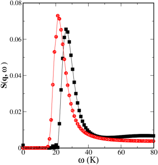
Figure 1: (Color online) Longitudinal component of the dynamic structure factor, $S({\bf q},\omega)$, for q = 0.83 r.l.u. along the [100] direction: single phonon contribution (circles, red online), and total structure factor (squares, black online). The lines are a guide to the eye.

In the simulations we used samples containing between 128 and 432 atoms. This allowed us to calculate $S({\bf q},\omega)$ for values of $q$ between 0.17 and 1 in relative lattice units (r.l.u.= 2$\pi/a$, where $a$ is the lattice parameter). The number density was set to $\rho=0.02854~{}(1/A^{3})$ and the temperature was $T=1.6~{}K$. A perfect bcc lattice was chosen as the initial configuration. The effects of Bose statistics are not taken into account in our simulation, which is a reasonable approximation for the solid phase. A typical example of the calculated dynamic structure factor is shown in Fig.1. The figure shows both the single phonon contribution $S_{1}({\bf q},\omega)$ and the total $S({\bf q},\omega)$ for a longitudinal phonon along the [001] direction. To illustrate the difference between $S_{1}({\bf q},\omega)$ and $S({\bf q},\omega)$, we chose to show the results for $\bf q$ close to the boundary of the Brillouin zone. This difference is discussed below.

III Results

III.1 Phonon spectra

The calculated longitudinal and transverse phonon spectra of solid ${}^{4}He$ in the bcc phase along the main crystal directions ([001], [111] and [011]) are shown in Figs. 2 - 7. We compare our results with the experimental data measured by inelastic neutron scattering from bcc ${}^{4}\text{H}e$ with a molar volume of 21.1 $\text{c}m^{3}$ at T = 1.6 K., by Osgood et al,Osgood ; Osgood1 ; Osgood2 and by Markovitch et al. Tuvi

Figure 2: (Color online) Calculated dispersion relation of the L[001] phonon branch (squares, red online) using $S_{1}({\bf q},\omega)$. Experimental data are from Osgood ; Osgood2 (triangles up) and from Tuvi (triangles down). The error bars represent statistical uncertainty.

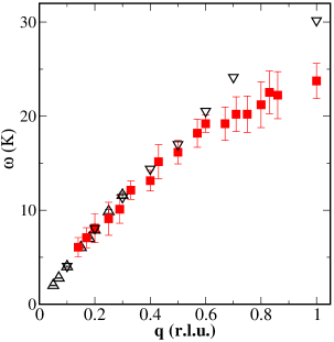
Figure 3: (Color online) Calculated dispersion relation of the T[001] phonon branch (squares, red online) using $S_{1}({\bf q},\omega)$. Experimental data are from Osgood ; Osgood2 (triangles up) and from Tuvi (triangles down). The error bars represent statistical uncertainty.

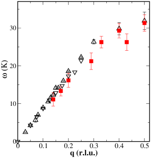
Figure 4: (Color online) Calculated dispersion relation of the L[011] phonon branch (squares, red online) using $S_{1}({\bf q},\omega)$. Experimental data are from Osgood ; Osgood2 (triangles up) and from Tuvi (triangles down). The error bars represent statistical uncertainty.

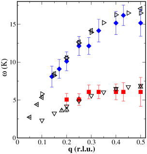
Figure 5: (Color online) Calculated dispersion relations of transverse phonon branches along [011] using $S_{1}({\bf q},\omega)$. Calculated values are shown for the $T_{1}$ branch (squares, red online) and $T_{2}$ branch (diamonds, blue online). Experimental data are from Osgood ; Osgood2 ( $T_{1}$-triangles up, $T_{2}$-triangles left) and from Tuvi ($T_{1}$-triangles down, $T_{2}$-triangles right). The error bars represent statistical uncertainty.

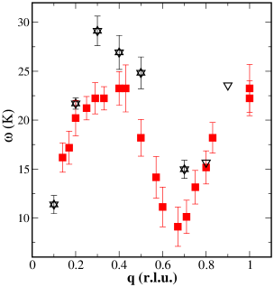
Figure 6: (Color online) Calculated dispersion relation of the L[111] phonon branch (squares, red online) using $S_{1}({\bf q},\omega)$. Experimental data are from Osgood ; Osgood2 (triangles up) and from Tuvi (triangles down).The error bars represent statistical uncertainty.

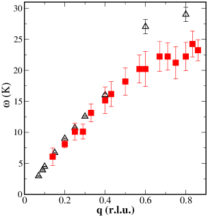
Figure 7: (Color online) Calculated dispersion relation of the T[111] phonon branch (squares, red online) using $S_{1}({\bf q},\omega)$. Experimental data are from Osgood ; Osgood2 (triangles up) and from Tuvi (triangles down). The error bars represent statistical uncertainty.

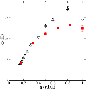
Figure 8: (Color online) Calculated dispersion relation of the L[001] phonon branch (squares, red online) using $S({\bf q},\omega)$. Experimental data are from Osgood ; Osgood2 (triangles up) and fromTuvi (triangles down). The error bars represent statistical uncertainty.

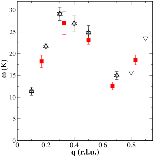
Figure 9: (Color online) Calculated dispersion relation of the L[111] phonon branch (squares, red online) using $S({\bf q},\omega)$. Experimental data are from Osgood ; Osgood2 (triangles up) and from Tuvi (triangles down). The error bars represent statistical uncertainty.

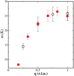
Figure 10: (Color online) A comparison of dispersion relations of the L[001] phonon branch obtained in the present work using $S({\bf q},\omega)$(squares, red online), with the same relation calculated by means of the Shadow Wave Function techniqueReatto (circles). The error bars represent statistical uncertainty.

As expected, the agreement between our simulations of $S_{1}({\bf q},\omega)$ and experiment is very good at small ${\bf q}$, where one-phonon excitation is the most significant contribution to $S({\bf q},\omega)$. As ${\bf q}$ increases, higher order processes become significant, and the calculated values deviate from the experimental data, especially along [001] and [111]. In the case of longitudinal phonons, it is possible to calculate their energies using the total $S({\bf q},\omega)$ obtained directly from Eq. (1) instead of just the single phonon contribution. The dispersion relations calculated with $S({\bf q},\omega)$ are shown in Figs. 8 and 9. It is evident that using the total scattering function improves the agreement with experiment at large ${\bf q}$, especially for the [111] direction.

We point out that the calculated phonon branches $T_{1}(110),T_{2}(110)$ and $L(110)$ show good fit to the experimental data. Our results were obtained with the two body potential, which takes the He atoms as point particles. Gov et al. Gov suggested that one needs to go beyond this approximation to obtain the $T_{1}(110)$ phonon branch in good agreement with experiment. Gov’s approach also predicts the new excitation branch observed recentlyEmil . Although the calculated $T_{1}(110)$ branch is in agreement with experiment without any additional assumptions, we were not able to see the new excitation in our simulations. Experimentally, this excitation is about an order of magnitude less intense than a phonon. It is best observed in scattering experiments done with very small $\bf q\leq$ 0.1 r.l.uTuvi . Both these factors make it very difficult to search for this excitation in simulations. Whether it can be found in this approach remains an open question.

In addition to experimental results, our simulations can also be compared with those of Galli and ReattoReatto , who used the Shadow Wave Function (SWF) approach to calculate the longitudinal phonon branches of bcc ⁴He. As shown in Fig.10, the overall agreement between these PIMC simulations and SWF results is good.

III.2 Vacancies

Recent experimental work Kim revived the interest in point defects, such as vacancies. It is therefore interesting to examine the influence of vacancies on the properties of the solid. We repeated our calculation of the phonon branches in the presence of 0.23$\%$ vacancies (1 atom of 432). Within the statistical error bars, we found no difference between the phonon energies with or without vacancies. Galli and ReattoReatto found that vacancies lower the energies of the phonons close to the boundary of the Brillouin zone. However, in their simulation they used a concentration of vacancies of 0.8$\%$, so that the cumulative effect may be larger. We also calculated the vacancy formation energy, $\Delta E_{v}$, according to Pederiva et al. Pederiva

$$\Delta E_{v}=(E(N-1,\rho)-E(N,\rho))(N-1),$$ (14)

where $E(N,\rho)$ is the total energy of $N$ atoms. The energy $E(N,\rho))$ was calculated for a perfect crystal, while $E(N-1,\rho)$ was calculated after removing one atom. The density of two systems was kept the same by adjusting the lattice parameter. Values of $\Delta E_{v}$ calculated using the PIMC, Shadow Wave Function (SWF) Chester and Shadow Path Integral Ground State (SPIGS)Reatto methods are summarized in Table 1. In addition, we calculated $\Delta E_{v}$ at constant volume, which is the condition usually realized in experiments rather than constant density. We obtained $\Delta E_{v}$= 5.7 $\pm$ 0.7 K. The lower value arises since the repulsive part of the potential is weaker in a sample having lower density. There is no generally accepted experimental value Burns of $\Delta E_{v}$. According to NMR studiesAllen ; Schuster the energy of vacancy formation in the bcc phase is $\Delta E_{v}=6.5\pm 0.2$(K), while X-ray studiesFraas suggest that $\Delta E_{v}=9\pm 1$(K). We comment here that the calculated values of $\Delta E_{v}$ are significantly smaller than 14K, the energy of the new excitation observed by Markovitch et al.Emil ; Tuvi . Hence, this new excitation does not seem to be a simple vacancy.

Table 1: Calculated energy of formation of a vacancy, $\Delta E_{v}$, for bcc solid ${}^{4}He$. N is the number of atoms used in each of the simulations.

source	method	density (1/$A^{3}$)	N	$\Delta E_{v}$ (K)
this work	PIMC	0.02854	128	$10.57\pm 0.38$
this work	PIMC	0.02854	250	$9.96\pm 0.89$
ref.Chester	SWF	0.02854	128	$8.08\pm 2.76$
ref.Chester	SWF	0.02854	250	$6.69\pm 3.86$
ref.Reatto	SWF	0.02898	128	$8.9\pm 0.3$
ref.Reatto	SPIGS	0.02898	128	$8.0\pm 1.3$

IV Conclusions

We calculated the dynamic structure factor for solid helium in the bcc phase using PIMC simulations and the MaxEnt method. PIMC was used to calculate the intermediate scattering function in the imaginary time from which the dynamic structure factor was inferred with the MaxEnt method. We extracted the longitudinal and transverse phonon branches from the one-phonon dynamic structure factor. To the best of our knowledge this is the first simulation undertaken for the transverse branches. At small ${\bf q}$, where the one-phonon excitation is the most significant contribution to the dynamic structure factor, the agreement between our simulations and experiment is very good. At large ${\bf q}$, multi-phonon scattering and interference effects Glyde becomes important. Consequently, the position of the peak of in the $S_{1}({\bf q},\omega)$ does not correspond to the position of the peak in the $S({\bf q},\omega)$, and the phonon energies calculated from $S_{1}({\bf q},\omega)$ are too low. If $S({\bf q},\omega)$ is used instead of $S_{1}({\bf q},\omega)$, the agreement with experiment is significantly improved. We repeated the simulations in the presence of 0.23$\%$ of vacancies, and found no significant differences in the phonon dispersion relations. We also calculated the formation energy of a vacancy both at constant density and at a constant volume.

- (1) H. R. Glyde , Excitations in Liquid and Solid Helium , Clarendon Press, Oxford, (1994).
- (2) H. Horner, J. Low. Temp. Phys. 8, 511, (1972).
- (3) N. Gov and E. Polturak, Phys. Rev. B , 60, 1019, (1999).
- (4) M. Boninsegni and D. M. Ceperley, J. Low. Temp. Phys. 104, 336, (1996).
- (5) D. E. Galli and L. Reatto, J. Low. Temp. Phys., 134, 121, (2004).
- (6) E. Kim and M. H. W. Chan, Science,305, 1941, (2004).
- (7) T. Markovich, E. Polturak, J. Bossy, and E. Farhi, Phys. Rev. Lett., 88, 195301, (2002).
- (8) T. Markovich, Inelastic-Neutron Scattering from bcc 4He, PhD. Thesis, Haifa, Technion, (2001).
- (9) B. Chaudhuri, F. Pederiva, and G. V. Chester, Phys. Rev. B., 60, 3271, (1999).
- (10) D. M. Ceperley, Rev. Mod. Phys., 67, 279, (1995).
- (11) K. Ohno, K. Esfarjam, Y. Kawazoe, Computational Material Science; From Ab Initio to Monte Carlo Methods, Springer, Berlin, 1999.
- (12) B. Bernu and D. M. Ceperley, Quantum Simulations of Complex Many-Body Systems: From Theory to Algorithms , NIC Series 10, Julich, 2002.
- (13) R. A. Aziz, A. R. Janzen, and M. R. Moldover, Phys. Rev. Let. 74, 1586 (1995).
- (14) M. Born and K. Huang, Dynamical theory of crystal lattices, Clarendon Press, Oxford, (1954).
- (15) P. Bruesch,Phonons, theory and experiments I : lattice dynamics and models of inter atomic forces , Berlin, Springer, (1982).
- (16) M. Jarrell and J. E. Gubernatis, Phys. Rep., 269, 133, (1996).
- (17) J. E. Gubernatis, M. Jarrell, R. N. Silver, and D. S. Sivia Phys. Rev. B 44, 6011, (1991).
- (18) E. B. Osgood, V. J. Minkiewicz, T. A. Kitchens, and G. Shirane, Phys. Rev. A 5, 1537 (1972).
- (19) E. B. Osgood, V. J. Minkiewicz, T. A. Kitchens, and G. Shirane, Phys. Rev. A 6, 526 (1972).
- (20) V. J. Minkiewicz, T. A. Kitchens, G. Shirane, and E. B. Osgood, Phys. Rev. A 8, 1513 (1973).
- (21) F. Pederiva, G. V. Chester, S. Fantoni, and L. Reatto, Phys. Rev. B 56, 5909, (1997).
- (22) C. A. Burns and J. M. Goodkind, J. Low. Temp. Phys., 95, 695, (1994).
- (23) A. R. Allen, M. G. Richards, and G. Sharter, J. Low. Temp. Phys., 47, 289, (1982).
- (24) I. Schuster, E. Polturak, Y. Swirsky, E. J. Schmidt, and S. G. Lipson, J. Low Temp. Phys. 103, 159, (1996).
- (25) B. A. Fraass, P. R. Granfors, and R. O. Simmons, Phys. Rev. B., 39, 124, (1989).