Formation of Liesegang patterns in the presence of an electric field

Abstract

The effects of an external electric field on the formation of Liesegang patterns are investigated. The patterns are assumed to emerge from a phase separation process in the wake of a diffusive reaction front. The dynamics is described by a Cahn-Hilliard equation with a moving source term representing the reaction zone, and the electric field enters through its effects on the properties of the reaction zone. We employ our previous results [I. Bena, F. Coppex, M. Droz, and Z. Rácz, J. Chem. Phys. 122, 024512 (2005)] on how the electric field changes both the motion of the front, as well as the amount of reaction product left behind the front, and our main conclusion is that the number of precipitation bands becomes finite in a finite electric field. The reason for the finiteness in case when the electric field drives the reagents towards the reaction zone is that the width of consecutive bands increases so that, beyond a distance $\ell_{+}$, the precipitation is continuous (plug is formed). In case of an electric field of opposite polarity, the bands emerge in a finite interval $\ell_{-}$, since the reaction product decreases with time and the conditions for phase separation cease to exist. We give estimates of $\ell_{\pm}$ in terms of measurable quantities and thus present an experimentally verifiable prediction of the ”Cahn-Hilliard equation with a moving source” description of Liesegang phenomena.

I Introduction

Precipitation patterns named after Liesegang liesegang1896 ; henisch91 have been investigated for more than 100 years. Their discovery came from work on photoemulsions liesegang1896 , and the interest in these patterns was sustained during all these years by recognizing that the underlying dynamics had connections to rather diverse physical- (e.g. near-equilibrium crystal growth krug ), geological- (formation of agates kruhl ), chemical- (pattern formation in reaction-diffusion systems swinney ) and more exotic (e.g. aggregation of asphaltene in crude oil Sheu2004 ) phenomena. From theoretical point of view, the Liesegang patterns enjoyed continuing attention since attempts at their explanations were testing the theories of precipitation processes Ostwald ; Wagner1950 ; Prager1956 (for a recent overview see Ref.antal98 ) and, furthermore, the phenomenon was considered as a highly-nontrivial example of pattern formation in the wake of a moving front Dee1986 ; cross94 .

The origin of recent attention to Liesegang patterns is the hope that the phenomena may be relevant in engineering of meso- and microscopic patterns Giraldo2000 ; Lebedeva2004 ; Fialkowski2005 . The novelty of the idea is that, in contrast to the ”top-down” processing (removing material in order to create a structure), the Liesegang dynamics provides a ”bottom-up” mechanism where the structure emerges from a bulk precipitation process Lebedeva2004 . Of course, many obstacles will have to be overcome before such a strategy succeeds, the main one being the problem of controlling the pattern generated by a reaction-diffusion process. It is known experimentally, with the results formulated in the Matalon-Packter law Matalon1955 , that some degree of control may be exercised through the appropriate choice of the concentrations of the inner and outer electrolytes participating in the process. It is also known, but much less understood, that the gel strongly influences the resulting patterns Toramaru2003 . Furthermore, recent experiments Fialkowski2005 indicate that the shape of the gel may be used in designing appropriate geometry in the precipitation patterns.

The methods of control described above are somewhat rigid since the parameters cannot be changed during the process while, ideally, one requires an easily tuned, flexible external field for control. In principle, the electric field provides such an external control and, indeed, there is experimental evidence happel29 ; kisch29 ; ortoleva78 ; sharbaugh89 ; das90 ; das91 ; das92 ; sultan00 ; sultan02 ; ghoul03 ; lagzi02 ; lagzi03 ; shreif04 that an electric field significantly alters the emerging pattern (see Fig.1 for a schematic experimental setup). Unfortunately, these experiments give only a qualitative picture about the effects of the electric field, and the theory is even less developed ortoleva78 ; ghoul03 ; lagzi02 ; lagzi03 ; Feeney-Orto1983 .

Our aim with this paper is to improve the theoretical description of electric field effects and to bring it up to the level of quantitative predictions. We have shown recently bena05 that there are problems with previous attempts ortoleva78 ; ghoul03 ; lagzi02 ; lagzi03 ; Feeney-Orto1983 which incorporate the electric field by assuming that it results in the drift of the reacting ions as well as in the drift of the reaction zone. Treating the background ions properly by using the electroneutrality condition, we found that the main effect of the field is that the amount of reaction product left behind the reaction zone increases (decreases) linearly in space depending whether the field drives the reacting ions towards (away) from the reaction zone. Building on these results, we shall show below using the ”Cahn-Hilliard equation with moving source” model antal99 ; antal01 , how the field affects the precipitation pattern itself.

The choice of the model must be explained since a century of research did not lead to a generally accepted theory of this pattern forming process. The reason is perhaps the complexity of the interplay between the motion of the reaction front and the precipitation dynamics of the reaction product (and the intermediate reaction steps that may also be present), thus preventing the creation of a single model encompassing all the possibilities. The approach we consider antal99 ; antal01 simplifies the situation by first treating the kinetics of reaction and the motion of the reaction front galfi88 ; cornell93 ; unger00 . Then, the reaction product generated by the front is inserted as a source in the phase separation process described by the Cahn-Hilliard equation gunton83 ; cahn58 ; cahn61 ; hohenberg77 . This theory has been shown antal99 ; antal01 ; racz99 ; droz00 ; magnin00 to generate Liesegang patterns which satisfy the time- and spacing-laws morse ; jabli (patterns emerging from most other theories do the same), the Matalon-Packter law Matalon1955 (significantly fewer theories can produce such patterns), and the width law Muller82 ; droz99 ; racz99 (no other theory yields this law since none of them has an underlying thermodynamics for setting the values of steady-state concentrations). This theory is also distinct from previous approaches in that it has a minimum number of parameters which can be related to experimentally measurable quantities and thus the theory can give quantitative predictions racz99 . We should also note that, depending on the motion of the front, the phase separation process may occur at the position of the front or well behind the front antal01 thus the model can also describe the limit of small imposed gradients Muller-Ross03 .

In order to summarize the results obtained from the above theory for the case of external field present, let us first describe the setup (Fig.1) more precisely. A chemical reagent $B\equiv(B^{+},B^{-})$, called inner electrolyte, is dissolved in a gel matrix inside a part of the small central cylinder (from point “$0$” to the right on the $x$-axis). A second reactant $A\equiv(A^{+},A^{-})$ (outer electrolyte), of much higher concentration, is brought in contact with the gel (at point “$0$” on the $x$-axis). The two reservoirs of electrolytes $A$ and $B$ are providing constant concentrations $a_{0}$ and $b_{0}$ ($a_{0}\gg b_{0}$) of the reagents at the two ends of the central cylinder. The outer electrolyte $A$ diffuses into the gel and reacts ($A^{-}+B^{+}\rightarrow C$) with the inner electrolyte $B$. The reaction front moves to the right and, under appropriate conditions, the reaction product $C$ precipitates, and one observes the emergence of bands of precipitate perpendicular to the direction of motion of the front. The reservoirs of electrolytes $A$ and $B$ are kept at a constant potential difference $U=V_{B}-V_{A}$, which corresponds to an average applied field intensity $E=-U/L$ inside the central cylinder of length $L$. Let us note that throughout this paper we shall call forward electric field a field that drives the reacting ions towards the reaction zone; in our setup this corresponds to a positive tension $U>0$, or to $E<0$. On the contrary, a field that works against the reacting ions reaching the reaction zone will be referred to as a reverse electric field, which in our setup corresponds to a negative tension $U<0$, or to $E>0$.

Figure 1: Schematic representation of the system under study. The inner electrolyte $B(B^{+},B^{-})$ is dissolved in a gel matrix inside a part of the small central cylinder (from point “$0$” to the left on the $x$-axis). The outer electrolyte $A(A^{+},\,A^{-})$, of much higher concentration, is brought in contact with the gel (at point “$0$” on the $x$-axis). The two reservoirs of electrolytes $A(A^{+},\,A^{-})$ and $B(B^{+},B^{-})$ assure constant concentrations $a_{0}$ and $b_{0}$ ($a_{0}\gg b_{0}$) of the ions at the two ends of the central cylinder. The outer electrolyte ions diffuse into the gel, where the reaction $A^{-}+B^{+}\rightarrow C$ takes place. (The background ions $A^{+}$ and $B^{-}$ do not react.) The reaction front moves without convection towards the right, and precipitation bands – i.e., the alternation of high-density-$C$ regions (shaded areas) and low-density-$C$ regions – emerge inside the cylinder in the wake of this moving reaction front. A tension $U=V_{B}-V_{A}$ is applied between the ends of the central cylinder of length $L$, which corresponds to an average applied field intensity $E=-U/L$. A positive tension $U>0$ (corresponding to $E<0$) drives the reacting ions towards the reaction zone (forward electrc field). A negative tension $U<0$ (corresponding to $E>0$) works against the reacting ions reaching the reaction zone (reverse electric field).

Without the external field ($U=0$), the positions of the bands ($x_{n}$, measured from the initial contact of the reagents) form a geometric series, $x_{n}\sim(1+p)^{n}$, where $1+p$ or $p>0$ is called the spacing coefficient. For small fields ($|E|=|U|/L\lesssim 2$ V/m, for which one has a ‘sufficient’ number of bands, i.e., $\geq 20$), the band spacing can still be described as geometric series and our first result pertains to the dependence of the effective spacing coefficient on the applied field, $p=p(U/L)$. We call it effective spacing coefficient because these geometric series are finite as evidenced by the results for higher fields. The reason for the finite number of bands for electric field that drives the reagents towards the reaction zone (called forward field in the following) is that the width of consecutive bands increases faster than the distance between the bands. Thus one finds that the precipitation is continuous (plug is formed) beyond a distance $\ell_{+}$. The number of band is also finite and they appear in an interval $[0,\ell_{-}]$ for the case of a field of reverse polarity. The reason for finiteness, however, is different. In case of a field working against the reacting ions reaching the reaction zone, the amount of reaction product generated in the reaction zone decreases with time and the conditions for phase separation cease to exist. The quantities $\ell_{+}$ and $\ell_{-}$ are easily accessible in experiments, and our main result (apart from qualitative observations) is that we give an estimate of them in terms of measurable quantities. Thus we provide a way of designing the spatial range of the emerging pattern. In view of the competing theories of Liesegang phenomena, this also gives yet another way of discovering which is the correct description.

Below we present the details in the following order. First, the Cahn-Hilliard equation and the changes in the source term in the presence of an electric field are discussed (Sec. II). Next (Sec. III), the results of numerical simulations and qualitative arguments concerning the characteristics of the Liesegang patterns for a forward applied field are presented. The case of the reverse polarity is described in Sec. IV. The comparison with experiments is discussed in Sec. V, while the conclusions and perspectives are given in Sec. VI. Finally, a discussion on the choice of the parameters of our theoretical model, as inferred from experimental data, can be found in the Appendix.

II Phase separation and dynamics of the reaction product $C$ in the presence of an external electric field

There is experimental evidence that the Liesegang pattern is an alternation of high-density $c_{h}$ and low-density $c_{l}$ regions of the precipitate $C$. Thus, the reaction product phase-separates behind the reaction front, and since this takes place on a macroscopic scale, its dynamics can be represented through an extension of the Cahn-Hilliard equation (in other contexts, this is the equation of model B of critical dynamics hohenberg77 ). This equation, however, requires the knowledge of the free energy density ${\cal F}$ of the system; note that for a homogeneous system, ${\cal F}$ has to present two minima in order to accommodate the two equilibrium states of high $c_{h}$ and low $c_{l}$ densities. The simplest form of ${\cal F}$ having this property and containing the minimum number of parameters (which, moreover, guarantees the stability of the system against short-wavelength fluctuations) is the Ginzburg-Landau free energy density

$${\cal F}[m]=-\frac{1}{2}\varepsilon m^{2}+\frac{1}{4}\gamma m^{4}+\frac{1}{2}\sigma(\nabla m)^{2}\,.$$ (1)

Here we introduced the ‘reduced’ concentration

$$m(x,t)=\frac{c(x,t)-(c_{h}+c_{l})/2}{(c_{h}-c_{l})/2}$$ (2)

that varies between $-1$ and $+1$ when the concentration of the product $C$ varies between $c_{l}$ and $c_{h}$. Note the underlying assumption of the one-dimensional character of the system, i.e., the fact that all the relevant parameters are only $x$-dependent, that is well-justified for the experimental setup in Fig. 1. The parameters $\varepsilon$, $\gamma$, and $\sigma$ are system and temperature dependent, with (i) $\varepsilon>0$ ensuring that the system is in the phase separating regime (i.e., the temperature is smaller than the critical one); (ii) $\gamma=\varepsilon$ in order to ensure that the minima of the free energy correspond to $m=\pm 1$ (the homogeneous high and low density phases of $C$); (iii) $\sigma>0$ in order to provide stability against short-wavelength inhomogeneities. Figure 2 offers a schematic representation of the homogeneous part of the free energy ${\cal F}$ as a function of $m$, with the different stability regions. Because the $C$-s are assumed to be neutral particles, the free energy density (i.e., the parameters $\varepsilon=\gamma$, $\sigma$, and $\lambda$) and the corresponding stability diagram are not modified by an external electric field.

\psfrag{F(m)}{{\Large${{\cal F}(m)}$}}\includegraphics[width=195.12767pt]{figure2.eps}

Figure 2: The homogeneous part of the free energy density ${\cal F}$ as a function of the reduced density $m$. The phase separation is an activated process in the metastable regimes $m_{s}=1/\sqrt{3}<|m|<m_{e}=1$, while it goes by spinodal decomposition in the linear instability region $|m|<m_{s}=1/\sqrt{3}$.

The dynamics of $C$ is thus driven by the free-energy density (1), but, in addition, there is a continuous creation of $C$ by the moving reaction front, with a certain space and time dependent source density. One is thus led to write down antal99 the following phenomenological evolution equation for the reduced concentration field $m(x,t)$:

$$\frac{\partial m}{\partial t} = -\lambda\Delta\frac{\delta{\cal F}[m]}{\delta m}+S_{m}(x,t)$$ (3)

$$= -\lambda\Delta(\varepsilon m-\gamma m^{3}+\sigma\Delta m)+S_{m}(x,t)\,,$$

where $\lambda$ is a kinetic coefficient and $S_{m}(x,t)$ is the source density. Equation (3) has to be solved with the homogeneous initial condition $m(x,t=0)=-(c_{h}+c_{l})/(c_{h}-c_{l})$ that corresponds to the absence of $C$ inside the system before the beginning of the reaction. Note that the above “Cahn-Hilliard equation with a source” should also contain two noise terms. One of them is the thermal noise, while the other one originates in the chemical reaction that creates the source term. However, as discussed in cornell93 , the noise in $A+B\rightarrow C$-type reaction fronts can be neglected in dimensions $d\geq 2$, while neglecting the thermal noise term means that an effective zero-temperature process is considered, and that the phase separation takes place only through a spinodal decomposition mechanism. This approximation is supported by the experimentally-known fact of the very long life of the formed patterns, which amounts to a very low ‘effective temperature’ of the system. The theory could be refined by including the thermal noise, since then the nucleation and growth processes would be also captured. The role of noise has been investigated for the fieldless case in antal01 , and its effects in the presence of an electric field will be the subject of a forthcoming paper. Here we shall remain within the deterministic framework corresponding to Eq. (3).

Let us now concentrate on the source term $S_{m}(x,t)$ in Eq. (3). As already mentioned, this term models the production of $C$ by the moving reaction front, and it is influenced by the presence of an external electric field. The effect of the electric field has been studied in detail in bena05 , and we summarize below the main results for the range of parameters that are relevant for typical experimental situations. One has to realize first that the reagents $A$ and $B$ are electrolytes which dissociate,

$$A\rightarrow A^{+}+A^{-}\,,\qquad B\rightarrow B^{+}+B^{-}\,,$$ (4)

and the basic reaction process is

$$A^{-}+B^{+}\rightarrow C\,,$$ (5)

while the ‘background’ ions $A^{+}$ and $B^{-}$ are not reacting. The modelling of the system in bena05 was based on several simplifying assumptions: (i) the one-dimensional character of the system (i.e., all the relevant parameters are only $x$-dependent); (ii) the complete dissociation of the electrolytes $A$ and $B$ into their respective ions (that allows to eliminate the dynamics of the neutral $A$-s and $B$-s from our description); (iii) infinite reaction rate and irreversibility of the basic reaction $A^{-}+B^{+}\rightarrow C$. This is justified by the fact that the characteristic reaction time-scale is much smaller than any time-scale connected with diffusion and precipitation (pattern formation), and leads to a point-like reaction zone; (iv) the electroneutrality approximation (the local charge density is zero on space scales that are relevant to pattern formation), whose applicability for the systems under study was discussed in detail in unger00 ; (v) we considered monovalent ions; (vi) finally, we assumed equal diffusion coefficients $D$ of the ions. As mentioned in bena05 , any of these assumptions may be relaxed without generating major changes of the conclusions of our study. The reaction-diffusion equations for the concentration profiles of the ions can be solved numerically (with boundary conditions that correspond to the presence of the two reservoirs of ions – of concentrations $a_{0}$ and $b_{0}$, respectively – at the ends of the reaction cylinder).

A first result refers to the motion of the point-like reaction zone; it is, to a good approximation, a diffusive motion,

$$x_{f}(t)=\sqrt{2D_{f}t}\,,$$ (6)

with a diffusion coefficient $D_{f}$ that is practically unaffected by the field intensity, i.e., it is given by its fieldless expression

$$\mbox{erf}\left(\sqrt{\frac{D_{f}}{2D}}\right)=\frac{(a_{0}/b_{0})-1}{(a_{0}/b_{0})+1}\,,$$ (7)

where $D$ is the common diffusion coefficient of the ions. Note that for a reverse field there is also a small drift component in the motion of the front. However, for the range of reverse fields and observation times we are considering, this drift component can be neglected.

The effect of the field is more significant in the production of $C$. As known antal98 , in the absence of the field the concentration of $C$-s left behind the front is a constant and its value $c_{0}$ is determined by the initial concentrations of the ions $a_{0}$ and $b_{0}$, and by their diffusion coefficients. In the particular case of equal diffusion coefficients $D$ of the ions, its value is given by:

$$c_{0}\approx a_{0}\,K\sqrt{2D/D_{f}}\,,$$ (8)

where $K\equiv(1+b_{0}/a_{0})(2\sqrt{\pi})^{-1}\,\exp(-D_{f}/2D)$, and the diffusion coefficient $D_{f}$ of the front is given by Eq. (7). For an infinite reaction rate, the corresponding source density for the production of $C$ (i.e., the density of production of $C$ per unit time) is a $\delta$ peak localized at the instantaneous position of the front $x_{f}(t)$,

$$S_{m}(x,t)=\frac{a_{0}\,K\,\sqrt{D}}{(c_{h}-c_{l})/2}\,\,\frac{\delta(x-x_{f}(t))}{\sqrt{t}}$$ (9)

whose amplitude decays in time as $\sim 1/\sqrt{t}$.

Consider now an external electric field applied to the system. For both polarities of the field, and for relatively small values of the field intensity (the so-called linear regime at which we shall limit our study in this paper), there is a linear variation of the concentration of $C$-s with $x$, with a slope that is proportional to the applied tension,

$$c(x)=c_{0}[1+(\eta\,U/L)x]\,,$$ (10)

as illustrated by Fig. 3. The parameter $\eta$ depends on the values of the other parameters (i.e., $a_{0}$, $b_{0}$, and $D$), and for the set of parameters in Fig. 3 one infers $\eta\approx 5$ V^-1. We should mention that the validity of this linear regime is wider for positive tensions (e.g., it may go up to $U/L\approx 10$ V/m for the system considered in Fig. 3) and less extended for negative tensions (e.g., up to $U/L\approx-2$ V/m for the system in Fig. 3); beyond these limits there is a relative error larger than $10$ % in approximating $c(x)$ by a linear profile with the initial slope.

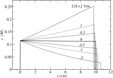
Figure 3: The density of the reaction product $C$ left behind the reaction front for different values of the electric field $U/L$ applied to the system. The observation time is $t=10$ days. The values of the other parameters are: $a_{0}=10$ M, $b_{0}=0.1$ M, and $D=10^{-9}$ m²/s, that lead to $c_{0}=0.1145$ M.

The above result on the spatial dependence (10) of the concentration of the reaction product is incorporated into the source term through the following modification of its amplitude:

$$S_{m}(x,t)=\frac{a_{0}\,K\,\sqrt{D}}{(c_{h}-c_{l})/2}\,\frac{[1+(\eta\,U/L)x]\,\delta(x-x_{f}(t))}{\sqrt{t}}\,.$$ (11)

As discussed in the Introduction, in the absence of an electric field ($U=0$) this spinodal decomposition scenario reproduces, in a simple and coherent way, all the generic laws of Liesegang patterns. Moreover, it contains very few parameters, which can be inferred from experimental data racz99 , and thus has a predictive power. We expect to recover these qualities in the presence of an applied external electric field, as well.

The solution to the Cahn-Hilliard equation (3) with the source (11), i.e., the profile of the reduced concentration $m(x,t)$ is obtained numerically. As already mentioned above and discussed in detail in bena05 , we decided to focus our analysis on the situations that are experimentally relevant and, in particular, the choice of parameters intends to mimic real experimental situations. Namely, we considered concentrations of the reagents $a_{0}$ and $b_{0}$ in the range $10^{-2}-10$ M, length $L$ of the system of some tenths centimetres, and tensions $U$ applied between system’s edges such that we are in the linear regime of the production of $C$, i.e., $U/L$ varies between $-2$ and $+10$ V/m. The common diffusion coefficient of the ions was chosen as $D=10^{-9}$ m²/s for all the calculations. The parameters $\lambda$, $\varepsilon=\gamma$, and $\sigma$ of the free-energy-driven part of the dynamics of $C$ can be inferred from the experimental data as explained in the Appendix. Finally, the pattern formation was followed for a period of the order of ten days of experimental observation time. In the following section we present the results that were obtained for a polarity $U>0$ of the applied field (the forward field), that favours the reaction, i.e., that drives the $A^{-}$ and $B^{+}$ ions towards the reaction zone. Section IV will be devoted to the $U<0$ (the reverse field) case study.

III Pattern characteristics for a forward applied field

A first generic feature of the patterns formed in the presence of the forward field ($U>0$ in our setup) is that the number of bands is finite, i.e., band formation stops at a certain moment through the appearance of a continuous precipitation region (a ‘plug’ of high-density precipitate). The higher the tension, the earlier this plug forms, see Fig. 4 for an illustration.

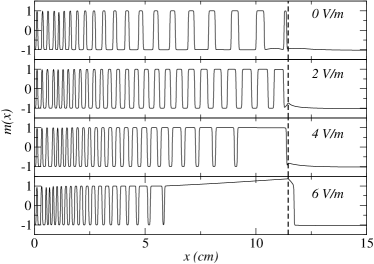
Figure 4: The profile of the reduced concentration $m(x)$ for different values of the forward applied field $U/L>0$. The snapshots are taken at $t=14$ days. The dashed lines represent the position of the reaction front at this time. The values of the other parameters are $c_{0}=0.1145\;M$, $c_{l}=0.0045\;M$, $c_{h}=0.3645\;M$, $D=10^{-9}$ m²/s, $D_{f}=5.43\cdot 10^{-9}$ m²/s, and $\eta=5$ V^-1. One notices the decrease in the band spacing with increasing tension, as well as the appearance of the plug – earlier for larger tensions.

One can make a rough estimate of the distance $\ell_{+}$ of the onset of the plug through the following reasoning: the plug forms when the width of the $n$-th high-density band, $w_{n}$, becomes equal to the distance $(x_{n+1}-x_{n})$ between the $n$-th and the $(n+1)$ high-density bands. If we estimate that the amount of $C$ produced by the front between $x_{n}$ and $x_{n+1}$ goes entirely in the $n$-th high-density band, i.e.,

$$c_{0}[1+(x_{n}+x_{n+1})/2](x_{n+1}-x_{n})=c_{h}\,w_{n}=c_{h}\,(x_{n+1}-x_{n})\,,$$ (12)

then we obtain for the distance $\ell_{+}=(x_{n}+x_{n+1})/2\approx x_{n}$:

$$\ell_{+}=\frac{L}{\eta U}\;\frac{c_{h}-c_{0}}{c_{0}}\,.$$ (13)

Figure 5 offers a comparison between the results of the numerical simulations and this theoretical estimation of $\ell_{+}$ for different values of the forward field $U/L>0$. Note that the experimental measurement of $\ell_{+}$ allows us to estimate the value of $c_{h}$ (provided that $c_{0}$ is known).

\psfrag{l}{{\Large$\ell$}}\includegraphics[width=195.12767pt]{figure5.eps}

Figure 5: The value of the distance $\ell_{+}$ of the plug-setting-in as a function of the forward applied field $U/L>0$. The diamonds represent the numerically estimated values, while the dashed line corresponds to the rough theoretical estimate, Eq.(13). The values of the parameters of the system are the same as for Fig. 4. The size of the symbols is representative for the estimated error bars.

A second generic feature of the pattern is that the distance between two successive bands diminishes as compared to the fieldless case, and this effect is increasing with increasing forward applied field $U/L$. This can be easily understood through a simple qualitative argument. In the presence of the forward field, the reaction front leaves behind a larger quantity of $C$ than in the absence of the field. Thus, after the formation of a band, the re-establishment of the phase-separation instability conditions takes place sooner in the presence of the field, resulting in a higher spatial density of bands in the system. With a good approximation, the positions of the bands $x_{n}$ still form a geometric series as in the fieldless case, and one can define an experimentally measurable ‘effective’ spacing-law parameter $p$:

$$x_{n}\sim(1+p)^{n}\,.$$ (14)

Thus, as illustrated in Fig. 6, $p$ is a decreasing function of the forward applied field $U/L$. Due to the decrease in the number of bands with increasing field intensity our measures of $p$ were restricted to a rather narrow interval of field intensities around $U/L=0$.

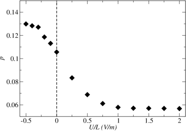
Figure 6: The value of the effective spacing coefficient $p$ as a function of the applied field $U/L$. The values of the parameters of the system are the same as for Fig. 4. The size of the symbols is representative for the estimated error bars.

Another remarkable feature of the pattern is its ‘instability’. Indeed, as illustrated by Fig. 7, due to the high densities of C in the plug region (which thus becomes unstable), there is a ‘flow-back’ of C from the plug towards the regions where the patterns had formed previously. Therefore, this may cause a gradual disappearance of some of the already formed bands. This effect is not present in the fieldless case.

Figure 7: The profile of the reduced concentration $m(x)$ at different times for a fixed forward applied field $U/L=6\;V/m$. The dashed lines represent the position of the reaction front at the corresponding times. One notices the progressive ‘flow-back’ of the $C$-s from plug zone, i.e., the backward disappearance of the pattern. The values of the parameters of the system are the same as for Fig. 4.

One has to realize that the structure of the patterns depends essentially on the position of the concentration of $C$-s left behind by the reaction front with respect to the stability domains associated with the free energy density ${\cal F}$. This remark holds both in the absence and in the presence of an applied field. If, for example, $c_{0}$ is below the spinodal value, no pattern will form in the absence of the field. However, in the presence of a forward field, the concentration of $C$-s left behind the front is continuously increasing, and thus, at a certain moment, it will cross the spinodal curve, and therefore the pattern formation mechanism will be ‘turned-on’, i.e., patterns will start to form after a certain time and then continue up to the eventual plug formation discussed above, as illustrated in Fig. 8a.

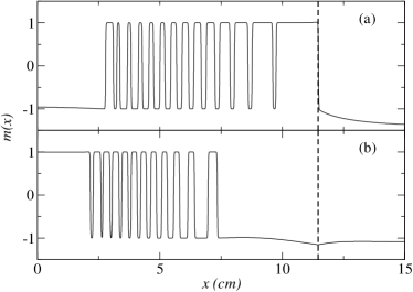
Figure 8: The profile of the reduced concentration $m(x)$ at $t=14$ days for two sets of values of the parameters: (a) $c_{0}=0.1145$ M, $D_{f}=5.43\cdot 10^{-9}$ m²/s, $\eta=5$ V^-1, $c_{h}=0.72$ M, and $c_{l}=0.120$ M (i.e., $c_{0}$ is below the spinodal decomposition domain), and an applied electric field $U/L=10$ V/m. One notices the initial absence of pattern, then a limited region of existence of the pattern and, in the end, a plug region starting to form. (b) $c_{0}=0.1145$ M, $D_{f}=5.43\cdot 10^{-9}$ m²/s, $\eta=5$ V^-1, $c_{h}=0.1045$ M, and $c_{l}=0.045$ M (i.e., $c_{0}$ is above the spinodal decomposition domain), and an applied electric field $U/L=-2$ V/m. One notices the initial plug region, then a limited region of existence of the pattern, and, in the end, the disappearance of the pattern. The dashed line represents the position of the front at the time of the snapshot.

We can also comment here on the width law Muller82 ; droz99 ; racz99 . As shown in racz99 , in the fieldless case the derivation of this law, $w_{n}\sim x_{n}^{\alpha}$, with $\alpha=1$, is straightforward. Let us apply the same reasoning as in racz99 in the presence of an electric field. One combines the facts that (i) the reaction front leaves behind a density $c(x)$ of $C$-s, Eq. (10); (ii) the $C$-s segregate into low ($c_{h}$) and high ($c_{h}$) density bands; (iii) the number of $C$-s is conserved in this segregation process. The equation expressing the conservation of $C$-s can be written as

$$c_{0}\left[1+(\eta U/L)(x_{n}+x_{n+1})/2\right](x_{n+1}-x_{n})=c_{h}w_{n}+c_{l}(x_{n+1}-x_{n}-w_{n})\,,$$ (15)

which together with $x_{n+1}=(1+p)x_{n}$ leads to

$$w_{n}=\frac{p(c_{0}-c_{l})}{c_{h}-c_{l}}\,x_{n}+\frac{c_{0}p(1+p/2)\eta U/L}{c_{h}-c_{l}}x_{n}^{2}\,.$$ (16)

It is however difficult to make a clear-cut statement on this point. Indeed, for field intensities for which the second term in (16) may start to play a role, the total number of bands is so small that no reliable conclusion can be drawn about the ‘systematic’ behaviour of their width. In case one attempts to fit $w_{n}\sim x_{n}^{\alpha}$, one will infer an effective $\alpha$ which is between $1$ and $2$ and which increases with the field.

IV Pattern characteristics for a reverse applied field

Let us consider now the case of the reverse polarity of the electric field (i.e., the case when it drives the reacting ions away from the reaction zone, $U<0$ in our setup). Again, a generic characteristic of the pattern is the finite number of bands. This can be easily understood in connection with the continuous decrease of the concentration of $C$-s left behind the reaction front, up to a point when the phase-separation conditions are no longer fulfilled. As illustrated in Fig. 9, there are less and less bands for larger and larger field intensities. But contrary to the forward field case, these bands are ‘stable’ i.e., nothing analogous to the ‘flow-back’ process in this case. Moreover, the last formed band collects progressively all the $C$-s left behind the front, i.e., its width increases slowly with time.

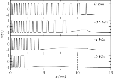
Figure 9: The profile of the reduced concentration $m(x)$ for different values of the reverse applied field $U/L<0$. The snapshots are taken at $t=14$ days. The dashed lines represent the position of the reaction front at this time (except for the last panel, where it indicates the stopping of the reaction, $S_{m}=0$). One notices the increase in band spacing with decreasing applied tension, as well as the rapid disappearance of the pattern. The values of the parameters of the system are the same as for Fig. 4.

There exists thus a maximum distance $\ell_{-}$ of the spatial extension of the pattern, which can be estimated experimentally as the right edge of the right-most high-density band. A rough theoretical estimation of this length is given through the condition that the concentration of the $C$ product at this point equals the lower limit of the spinodal decomposition domain, i.e.,

$$c(\ell_{-})=c_{l}+\left(1-\frac{1}{\sqrt{3}}\right)\,\frac{c_{h}-c_{l}}{2}\,,$$

from which

$$\ell_{-}=\frac{L}{\eta|U|}\;\frac{(c_{0}-c_{l})-(1-1/\sqrt{3})(c_{h}-c_{l})/2}{c_{0}}\,.$$ (17)

A comparison of this result with the numerical simulations is given in Fig. 10 for different values of the field intensity $|U|/L$.

\psfrag{l(cm)}{{\Large$\ell_{-}$ (cm)}}\includegraphics[width=195.12767pt]{figure10.eps}

Figure 10: The value of the distance $\ell_{-}$ of disappearance of the pattern as a function of the absolute value of the reverse applied field $|U|/L$. The diamonds represent the numerically estimated values, while the dashed line corresponds to the rough theoretical estimate, Eq.(17). The values of the parameters of the system are the same as for Fig. 4. The size of the symbols is representative for the estimated error bars.

We can see that the expressions for the two lengths $\ell_{+}$ and $\ell_{-}$ (Eqs. (13) and  (17)) provide a way to evaluate $c_{h}$ and $c_{l}$ through experimental measurements of the length of the patterns.

As expected, in the reverse field case, there is an increase of the spacing between the bands (as compared to the fieldless case), and this is illustrated by an increasing of the effective spacing coefficient $p$ with increasing field intensity $|U|/L$, see Fig. 6 for a numerical estimation.

Finally, it is worth mentioning again how the appearance of the pattern is sensitive to the position of $c_{0}$ with respect to the stability domains associated with the free energy density ${\cal F}$. If, e.g., $c_{0}$ is above this instability domain, there is no pattern formation in the fieldless case, but just a uniform plug of $C$ behind the front. However, as illustrated in Fig. 8b, in the presence of a reverse field, due to the continuous decrease in the concentration of $C$, the instability domain may be reached from above, and a pattern starts to form after an initial plug region, and eventually, as discussed above, stops after some time, when the instability domain is left for too small concentrations of $C$.

V Comparison with experiments

Experiments on Liesegang patterns in the presence of an electric field have been going on quite a while since the pioneering works of Happel et al. happel29 and Kisch kisch29 , see ortoleva78 ; Feeney-Orto1983 ; sharbaugh89 ; das90 ; das91 ; das92 ; sultan00 ; sultan02 ; ghoul03 ; lagzi02 ; lagzi03 ; shreif04 . As already mentioned in bena05 , with the exception of sharbaugh89 ; lagzi02 ; lagzi03 , these experiments were carried on for a single polarity of the electric field (i.e., either a ‘forward’, or a ‘reverse’ field according to our terminology).  It is therefore not surprising that each of them ‘covers’ only a part of the situations that are predicted by our theory, which thus has the merit to include all these elements in an unifying, coherent, and simple frame. We shall present below a brief qualitative summary of these experimental results.

Concerning the motion of the front, it is experimentally found to be diffusive in sharbaugh89 , das90 (with a slight decrease in the diffusion coefficient with increasing field intensity), and das91 (for a $2D$ geometry), in agreement with our theoretical predictions bena05 for a forward field. Other experiments sultan00 ; sultan02 ; ghoul03 , present a motion of the front with a small drift component (that increases with increasing field intensity sharbaugh89 ). Occasionally, this drift component is given a theoretical justification on the basis of a reaction-diffusion model for the system with a superimposed constant electric field intensity, see ghoul03 ; lagzi02 ; lagzi03 ; Feeney-Orto1983 – that, as discussed in bena05 , is a somewhat unrealistic assumption. Here again our model is able to capture the appearance of this small drift component for the case of a reverse electric field.

Several experimentally-studied modifications of the characteristics of the Liesegang patterns in the presence of an electric field are quoted in the literature, and sometimes they seem contradictory:
(i) A first striking observation is the appearance of an uniform precipitation for sufficiently high field-intensities ortoleva78 ; sharbaugh89 ; das90 ; das91 and/or after a sufficiently long time sharbaugh89 .
(ii) Also, there is an ‘acceleration’ of the band formation sharbaugh89 , i.e., the time of appearance of the first band decreases with increasing field intensity das91 .
(iii) A decrease of the spacing between successive bands (as compared to the fieldless case) with increasing field intensity is registered in ortoleva78 ; das91 .
(iv) On the other hand, an increase of the spacing between successive bands is described in sultan00 ; sultan02 ; ghoul03 , and shreif04 (for a $2D$ experimental setup).
(v) As reported in sultan00 ; sultan02 ; shreif04 , at a given time there are less bands formed for higher field intensities.
(vi) The paper das91 indicates a reduction of the initial “diffuse portion” with increasing field intensity, and shreif04 also gives an example of the reduction of the initial “fuzzy zone”.

One is now in position to recognize that all these features are recovered in a simple way within our theory. More precisely, (i)-(iii) and the first result in (vi) are obtained in our model in the case of a forward electric field, see Section III; while (iv), (v), and the second result in (vi) can be obtained theoretically for a reverse applied field, see Section IV.
(vii) Finally, a special remark on the results of lagzi02 ; lagzi03 , which sometimes match our results, sometimes are just the opposite of those obtained from our theory (as far as the polarity of the electric field is concerned). In particular, in lagzi02 it was found that (a) the motion of the reaction front is diffusive for a reverse field and has a small drift component for a forward field (contrary to our theory); (b) the average spacing coefficient $p$ decreases with increasing field (just like in our theory). In lagzi03 an attempt to fit the width law (see, e.g., racz99 ) in the presence of an electric field, $w_{n}\sim x_{n}^{\alpha}$, leads to an exponent $\alpha$ that is decreasing monotonically with the field – in opposition with the result of our discussion following Eq. (16). However it was argued lagzi04 that in his case the properties of the intermediate compounds are responsible for this ‘anomalous’ behaviour, and such effects are outside the range of our theoretical model.

Most of the above examples show agreement with our theory at a qualitative level. It should be noted however that our model offers quantitative estimates of the changes as compared to the fieldless case, and thus is well-suited for direct comparison with the results of appropriately-designed experiments.

VI Conclusions and perspectives

In this paper we examined the influence of an applied electric field on the formation and characteristics of Liesegang patterns that appear in the wake of an $A^{-}+B^{+}\rightarrow C$ reaction front. The appearance of the pattern is related to the phase separation of the precipitate $C$ into a high and a low density phase. At a macroscopic, phenomenological level, the dynamics of $C$ particles can be modelled using a Cahn-Hilliard equation supplemented with a space and time-dependent source term that describes the production of $C$-s by the reaction front. It was found that for both polarities of the applied field the pattern has a finite spatial extension. Moreover, measuring this spatial extension for various values of the applied tensions allows to infer the values of the concentrations of $C$ in the high and low density phases. The distance between the bands in the pattern is influenced by the intensity of the applied field, namely it decreases with increasing $U/L$ for a forward field $U>0$, and increases with increasing $|U|/L$ for a reverse field $U<0$.

One has to underline that the proposed model contains a minimal number of parameters, and all of them can be inferred from experimental data. Thus the model, besides reproducing well the generic experimental laws of Liesegang patterns, has a clear predictive power that can be used to control experimental situations. The data we are presenting are the result of numerical simulations, and are based on a set of simplifying assumptions. It is expected that most of these assumptions do not affect our main conclusions. However, the details of the reaction process leading to the final precipitate $C$ may be more complex (e.g., implying several steps, intermediate compounds with different electric charges and diffusivities, etc.), and the role of the electric field may also have unexpected features. The simplest extension of our work would be to consider a reaction scheme with one bivalent and two monovalent ions, a case that occurs in several experiments. Work on this type of systems is in progress.

Appendix A Setting the parameters

Typical experimental situations correspond to concentrations $a_{0}$ and $b_{0}$ of the reagents of the order of $10^{-2}-10$  M, with a ratio $a_{0}/b_{0}\sim 10-100$, and thus it is suitable to choose the unit of concentration as $n_{0}=1$ M. The diffusion coefficients of the reagents are of the order $\sim 10^{-9}$ m²/s, so that the length $\ell$ and time $\tau$ scales should be chosen such that $\ell^{2}/\tau$ is of the same order of magnitude,

$$\frac{\ell^{2}}{\tau}\sim D\,.$$

Moreover, the experimental patterns have a total length of about $20$ cm, and the time to produce such a pattern is of some tenth days – and this offers the order of magnitude of the diffusion coefficient of the reaction front, which is typically of the same order or an order of magnitude larger than the diffusion coefficients of the reagents (depending on the ratio $a_{0}/b_{0}$ of the concentration of the reagents). The typical widths of the precipitation bands are of a few mm at the beginning, and approach $\sim 1$ cm at the end, and so are the distances between two successive bands. From the visual observation of the beginning of the band formation it takes some tenth minutes for the band to be clearly seen, and some hundred minutes for its complete formation. Since the Cahn-Hilliard model has intrinsic length scale $\sqrt{\sigma/\varepsilon}$ and time scale $\sigma/(\lambda\varepsilon^{2})$, these have to be comparable to the typical length and time scales of the appearance of a single band. We are thus led to the following orders of magnitude for the length and time scales:

$$\ell=\sqrt{\sigma/\varepsilon}\sim 10^{-4}\,\mbox{m}\,,\quad\tau=\sigma/(\lambda\varepsilon^{2})\sim 10\,\mbox{s}\,.$$

There remains, however, the question of determining the concentrations of the two phases of the $C$ precipitate, $c_{h}$ and $c_{l}$. As explained in the main text, this can be done through measurements of the total spatial extent of the pattern in the presence of a forward, respectively reverse electric field.

Here is the set of parameters that we used in most of the simulations presented above. For the concentrations of the reagents we take $a_{0}=10$ M, $b_{0}=0.1$ M, and the common diffusion coefficient of the electrolyte ions is $D=10^{-9}$ m²/s. This leads, according to Eqs. (7) and (8), to a diffusion coefficient of the front $D_{f}=5.43\cdot 10^{-9}$ m²/s, and a concentration of the fieldless reaction product $c_{0}=0.1145$ M. For the above parameters the coefficient $\eta$ in the expression (10) of $c(x)$ is $\eta=5$ V^-1 . The parameters of the Cahn-Hilliard model are chosen such that $\ell=\sqrt{\sigma/\varepsilon}=10^{-4}$ m, and $\tau=\sigma/(\lambda\varepsilon^{2})=40$ s. Regarding the concentrations of the low and high density phases of $C$, we usually set them such that $c_{0}$ given above is in the instability domain of spinodal decomposition, $c_{h}=0.3645$ M, and $c_{l}=0.0045$ M.

- (1) R. E. Liesegang, Naturwiss. Wochenschr. 11, 353 (1896).
- (2) H. K. Henisch, Periodic Precipitation (Pergamon, New York, 1991).
- (3) J. Krug, Statistical physics of growth processes, pp. 1–62 in Scale Invariance, Interfaces and Non-Equilibrium Dynamics, M. Droz, A. J. McKane, J. Vannimenus, and D.E. Wolf (Eds.), Nato-ASI Series, Plenum, New-York (1995).
- (4) H.-J. Krug and J.-H. Kruhl (Eds.), Non-Equlibrum Processes and Dissipative Structures in Geoscience, Duncker and Humblot, Berlin (2001)
- (5) H. L. Swinney, Emergence and evolution patterns, pp 51–74, Princeton University Press (1996).
- (6) F. Arteaga-Larios, E.Y. Sheu, and E. Pérez, Energy and Fuels 18, 1324-1328 (2004).
- (7) W. Ostwald, Lehrbuch der allgemeinen Chemie, Engelman edt., Leipzig (1897).
- (8) C. Wagner, J. Colloid. Sci. 5, 85 (1950).
- (9) S. Prager, J. Chem. Phys. 25, 279 (1956).
- (10) T. Antal, M. Droz, J. Magnin, Z. Rácz, and M. Zrinyi, J. Chem. Phys. 109, 9479 (1998).
- (11) G. T. Dee, Phys. Rev. Lett. 57, 275 (1986).
- (12) For a review, see M. C. Cross and P. C. Hohenberg, Rev. Mod. Phys. 65, 851 (1994).
- (13) O. Giraldo, Nature 405, 38 (2000).
- (14) M. I. Lebedeva, D. G. Vlachos, and M. Tsapatsis, Phys. Rev. Lett. 92, 088301 (2004).
- (15) M. Fialkowski, A. Bitner, and A. Grzybowski, Phys. Rev. Lett. 94, 018303 (2005).
- (16) R. Matalon and A. Packter, J. Colloid Sci. 10, 46 (1955); A. Packter, Kolloid Z. 142, 109 (1955).
- (17) A. Toramaru, T. Harada, and T. Okamura, Physica D 183, 133-140 (2003).
- (18) P. Happel, R. E. Liesegag, and O. Mastbaum, Kolloid Z. 48, 80 (1929); ibid., 48, 252 (1929).
- (19) B. Kisch, Kolloid Z. 49, 154 (1929).
- (20) P. Ortoleva, Selected Topics from the Theory of Nonlinear Physico-Chemical Phenomena, pp. 236–288 in Theoretical Chemistry, Vol. IV, H. Eyring (Ed.), Academic Press, New York (1978).
- (21) A. H. Sharbaugh III and A. H. Sharbaugh Jr., J. Chem. Educ. 66, 589 (1989).
- (22) I. Das, A. Pushkarna, and A. Bhattacharjee, J. Phys. Chem. 94, 8968 (1990).
- (23) I. Das, A. Pushkarna, and A. Bhattacharjee, J. Phys. Chem. 95, 3866 (1991).
- (24) I. Das, A. Pushkarna, and S. Chand, J. Coll. Int. Sci. 150, 178 (1992).
- (25) R. Sultan and R. Halabieh, Chem. Phys. Lett. 332, 331 (2000).
- (26) R. F. Sultan, Phys. Chem. Chem. Phys. 4, 1253 (2002).
- (27) M. Al-Ghoul and R. Sultan, J. Phys. Chem. A 107, 1095 (2003).
- (28) I. Lagzi, Phys. Chem. Chem. Phys. 4, 1268 (2002).
- (29) I. Lagzi and F. Izsák, Phys. Chem. Chem. Phys. 5, 4144 (2003).
- (30) Z. Shreif, L. Mandalian, A. Abi-Haydar, and R. Sultan, Phys. Chem. Chem. Phys. 6, 3461 (2004).
- (31) R. Feeney, S.L. Schmidt, P. Strickholm, J. Chadam, and P. Ortoleva, J. Chem. Phys. 78 1293 (1983).
- (32) I. Bena, F. Coppex, M. Droz, and Z. Rácz, J. Chem. Phys. 122, 024512 (2005).
- (33) T. Antal, M. Droz, J. Magnin, and Z. Rácz, Phys. Rev. Lett. 83, 2880 (1999).
- (34) T. Antal, M. Droz, J. Magnin, A. Pekalski, and Z. Rácz, J. Chem. Phys. 114, 3770 (2001).
- (35) L. Gálfi and Z. Rácz, Phys. Rev. A 38, 3151 (1988).
- (36) S. Cornell and M. Droz, Phys. Rev. Lett. 70, 3824 (1993).
- (37) T. Unger and Z. Rácz, Phys. Rev. E 61, 3583 (2000).
- (38) J. D. Gunton, M. San Miguel, and P. S. Sahini, in Phase Transitions and Critical Phenomena, Vol. 8, The Dynamics of First-order Transitions, Eds. C. Domb and J. L. Lebowitz (Academic Press, New York, 1983).
- (39) J. W. Cahn and J. E. Hilliard, J. Chem. Phys. 28, 258 (1958).
- (40) J. W. Cahn, Acta Metall. 9, 795 (1961).
- (41) P. C. Hohenberg and B. I. Halperin, Rev. Mod. Phys. 49, 435 (1977).
- (42) See, e.g., Z. Rácz, Physica A 274, 50 (1999).
- (43) M. Droz, J. Stat. Phys. 101, 509 (2000).
- (44) J. Magnin, Ph.D. Thesis, University of Geneva (2000).
- (45) Harry W. Morse and George W. Pierce: Diffusion and Supersaturation in Gelatine, Proceedings of the American Academy of Arts and Sciences, 38 625-647 (1903)
- (46) K. Jablczynski, Bull. Soc. Chim. France 33, 1592 (1923).
- (47) S. C. Müller, S. Kai, and J. Ross, J. Phys. Chem. 86, 4078 (1982).
- (48) M. Droz, J. Magnin, and M. Zrinyi, J. Chem. Phys. 110, 9618 (1999).
- (49) S. C. Müller and J. Ross, J. Phys. Chem. A107, 7997 (2003)]. Note that Fig.9 of this paper indicates that the bands and the interband regions have constant (in space) densities, a prediction of the Cahn-Hilliard approach, and a condition for the width law to hold.
- (50) I. Lagzi, private communication.