Finite-size-scaling analysis of the $XY$ universality class between two and three dimensions: An application of Novotny’s transfer-matrix method

Abstract

Based on Novotny’s transfer-matrix method, we simulated the (stacked) triangular Ising antiferromagnet embedded in the space with the dimensions variable in the range $2\leq d\leq 3$. Our aim is to investigate the criticality of the $XY$ universality class for $2\leq d\leq 3$. For that purpose, we employed an extended version of the finite-size-scaling analysis developed by Novotny, who utilized this scheme to survey the Ising criticality (ferromagnet) for $1\leq d\leq 3$. Diagonalizing the transfer matrix for the system sizes $N$ up to $N=17$, we calculated the $d$-dependent correlation-length critical exponent $\nu(d)$. Our simulation result $\nu(d)$ appears to interpolate smoothly the known two limiting cases, namely, the KT and $d=3$ $XY$ universality classes, and the intermediate behavior bears close resemblance to that of the analytical formula via the $1/N$-expansion technique. Methodological details including the modifications specific to the present model are reported.

I Introduction

In analytical approaches, the spatial dimension $d$ is treated as a continuously variable parameter, and correspondingly, various quantities such as the critical indexes are expressed explicitly in terms of the parameter $d$. Such an approach allows us to see how the criticality changes from the classical (meanfield like) one as the spatial dimension deviates from an either lower or upper critical dimension gradually. However, it is not quite obvious that such an analytical formula could be justified (realized) by actual first-principles simulations (and hopefully by experiments) with respect to realistic lattice models. In fact, in conventional computer-simulation approaches, one has to fix the (embedding) spatial dimension to a certain integral value, and thus the analysis on criticality has been restricted to the integral values of $d$ inevitably.

An attempt to circumvent such a restriction was made by Novotny Novotny90 ; Novotny92 ; Novotny93a ; Novotny93b . His approach stems on a very formal expression for the transfer matrix so that the embedding spatial dimension can be varied continuously. (We explain his method in the next section. As anticipated naturally, this method is also of use in studying high dimensional ($d\geq 3$) systems. We refer readers to the references Novotny90 ; Nishiyama04 for this development.) Based on this formulation, he performed an extensive computer simulation, and surveyed the criticality of the Ising ferromagnet for $1\leq d\leq 3$. Astonishingly enough, he found that the numerical result is well described by both the $1+\epsilon$ and $4-\epsilon$ expansion formulas. In other words, his result clarifies that the analytical formulas for fractional values of $d$ are meaningful in the sense that they are reproduced by the first-principles-simulation scheme. (Strictly speaking, he utilized two distinctive approaches to control the embedding spatial dimension. In Ref. Novotny92 , he varies the “connectivity” of the lattice, whereas in Refs. Novotny93a ; Novotny93b , he twists the boundary condition to control the magnetic-domain-wall undulations.) Here, we stress that the Novotny approach is not a mere dimensional interpolation (crossover) that has been studied extensively in the past study Landau95 ; Ruge95 .

In this paper, we apply Novotny’s method to the “stacked” triangular Ising antiferromagnet Landau83 ; Kitatani83 ; Miyashita91 ; Queiroz95 ; Miyashita97 ; Blankschtein84 ; Heinonen89 ; Yamada90 ; Netz91 ; Bunker93 ; Gaulin95 ; Plumer93 ; Plumer95 ; Dantchev04 embedded in the space with the variable dimensions $2\leq d\leq 3$. Because of its $Z_{6}$ invariance, the model should exhibit the $XY$ universality class at the magnetic transition point Jose77 ; Tobochnik82 ; Rujan81 ; Challa86 ; Irakliotis93 . Our aim is to examine whether his method is applicable to generic problems other than the Ising universality class. We calculate the $d$-dependent correlation-length critical exponent. Thereby, we will show that the simulation result is comparable with the analytical $1/N$-expansion result up to O$(1/N)$ Ma72 ; Abe72 ; Suzuki72 ; Ferrel72 .

In fairness, it has to be mentioned that the critical phenomena for non-integer dimensions were studied extensively in the past Gefen84 ; Lin86 ; Taguchi87 ; Costa87 ; Hao97 . In these works, the authors set up their lattice models on a fractal structure (the Sierpinski gasket) in order to realize a magnetism in the fractional spatial dimensions. Here, we stress that in our approach, the spatial dimension can be varied continuously within a range.

The rest of this paper is organized as follows. In the next section, we explain how we constructed the transfer matrix for the stacked triangular antiferromagnet in $2\leq d\leq 3$. In Sec. III, we present the numerical results. Managing an extended finite-size scaling analysis, we estimate the correlation-length critical exponent in the range $2\leq d\leq 3$. In the last section, we present summary and discussions.

II Construction of the transfer matrix for the “stacked” triangular antiferromagnet in $2\leq d\leq 3$

In this section, we set up the transfer matrix formalism to simulate the “stacked” triangular antiferromagnet embedded in the dimensions $2\leq d\leq 3$. Our formalism is based on Novotny’s idea Novotny90 , with which he studied the Ising ferromagnet on (hyper) cubic lattices; in our preceding paper Nishiyama04 , we adopted his idea to the $d=3$ Ising ferromagnet with plaquette-type interactions. Before going into details, we first set up a basis of our scheme; namely, we dwell on the particular $d=3$ case. Then, we extend this preliminary basis to incorporate the embedding-spatial-dimension variation. We will also provide a number of technical modifications to improve the efficiency of the numerical simulation.

We decompose the transfer matrix into the following two contributions,

$$T=T^{\perp}\odot T^{\parallel},$$ (1)

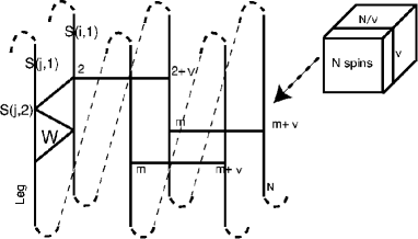
Figure 1: A schematic drawing of the construction of the transfer matrix for the “stacked” triangular antiferromagnet. Our scheme is based on Novotny’s idea Novotny90 . The sheet of triangular antiferromagnet extends along the “leg.” The leg is folded into a rectangular shape: To be specific, with use of the translation operator $P^{v}$ ($v$: interaction distance), we build a bridge between the $v$th neighbor spins along the leg.

where the symbol $\odot$ denotes the Hadamard (element by element) matrix multiplication; note that the multiplication of local Boltzmann factors yields the global Boltzmann weight. As explained below (see also Fig. 1 for the geometrical structure of our finite-size cluster), the decomposed parts $T^{\perp}$ and $T^{\parallel}$ account for the contributions from the intra and inter plane (triangular lattice) interactions, respectively.

First, let us consider the component $T^{\parallel}$. The matrix elements are given by the formula,

$$T^{\parallel}_{ij}=\langle i|A|j\rangle=W^{S(j,1)S(j,2)}_{S(i,1)S(i,2)}W^{S(j,2)S(j,3)}_{S(i,2)S(i,3)}\cdots W^{S(j,N)S(j,1)}_{S(i,N)S(i,1)},$$ (2)

where the indexes $i$ and $j$ specify the Ising spin configuration for both sides of the transfer-matrix slice; see Fig. 1. More specifically, we consider $N$ spins for the transfer-matrix slice, and the index $i$ denotes a spin configuration $\{S(i,1),\dots,S(i,N)\}$ arranged along the “leg.” The factor $W^{S_{3}S_{4}}_{S_{1}S_{2}}$ stands for the local Boltzmann weight for a unit cell of the triangular lattice with the corner spins $\{S_{1},S_{2},S_{3},S_{4}\}$. Explicitly, it is given by the following form,

$$W^{S_{3}S_{4}}_{S_{1}S_{2}}=\exp\left[-\frac{1}{T}\left(\frac{J}{2}(S_{1}S_{2}+S_{2}S_{4}+S_{4}S_{3}+S_{3}S_{1})+JS_{1}S_{4}\right)\right].$$ (3)

(The denominator of the coupling constant is intended to avoid double counting.) Here, the parameter $T$ denotes the temperature, and the parameter $J$ stands for the intra-plane antiferromagnetic interaction constant. Hereafter, we choose $J$ as the unit of energy; namely, we set $J=1$. It is to be noted that the component $T^{\parallel}$ (with $T^{\perp}$ ignored) leads to the transfer-matrix for a sheet of triangular antiferromagnet. In other words, the remaining component $T^{\perp}$ should raise the dimensionality to $d=3$ through introducing the inter-plane interactions. This is an essential idea of the Novotny method Novotny92 .

Second, we consider the component $T^{\perp}$ that accounts for the inter-plane interaction. The explicit matrix elements are given by the following formula,

$$T^{\perp}_{ij}=\langle i|BP^{v}|i\rangle,$$ (4)

with the interaction distance $v$. The matrix $B$ is given by the formula,

$$\langle i|B|j\rangle=W_{S(i,1)S(j,1)}^{\perp}W_{S(i,2)S(j,2)}^{\perp}\cdots W_{S(i,3)S(j,3)}^{\perp},$$ (5)

with $W_{S_{1}S_{2}}^{\perp}=\exp(-jS_{1}S_{2}/T)$ and the inter-plane interaction $j$. The matrix $P$ denotes the translational operator: That is, with one operation of $P$, a spin arrangement $\{S(i,m)\}$ shifts to $\{S(i,m+1)\}$; note that the periodic boundary condition is imposed. An explicit representation of $P$ is given in our preceding paper Nishiyama04 . Because of the insertion of $P^{v}$, the interaction $B$ bridges the $v$th neighbor pairs along the leg, and so it brings about the desired inter-plane interactions. As a matter of fact, in Fig. 1, we notice that the alignment of spins is folded into a rectangular shape with the edge lengths $v$ and $N/v$. It is an essential idea of Novotny that the operation $P^{v}$ is still meaningful, although the power $v$ is not an integral value. This rather remarkable fact renders freedom that one can construct the $d=3$ transfer-matrix systematically with arbitrary number of spins $N$.

Based on the above formalism, we readily simulate the stacked triangular antiferromagnet in $d=3$. In the following, we propose a scheme to tune the embedding spatial dimension continuously. Moreover, we will also provide a number of technical modifications, aiming to improve the efficiency of the simulation.

There are two controllable parameters for the dimension variation. That is, the inter-plane interaction $j$ and the interaction distance $v$: Apparently, the limit $j\to 0$ reduces the system to a sheet of triangular lattice. On the other hand, for large $v$, the stack width $N/v$ decreases, and eventually, at $v=N$, the system reduces to a sheet of triangular lattice as well; note the identity $P^{N}=1$ owing to the periodic boundary condition. In this paper, we adopt the former scheme. Namely, we will tune the parameter $j$, fixing the interaction distance $v$ to a moderate value $v=0.27N$. This choice is based on our observation that the finite-size-scaling behaviors become quite systematic for $v\approx N/n$ ($n$: integer), particularly at $n=4$.

Lastly, let us explain a number of technical modifications to improve the efficiency of the simulation: We propose the following replacement,

$$T^{\perp}_{ij}=\langle i|BP^{v}|i\rangle\to T^{\perp}_{ij}(v)=\langle i|BP^{v}|i\rangle\langle i|P^{-v}B|i\rangle.$$ (6)

(Note that correspondingly, we need to replace the temperature $T$ with $2T$ in order to compensate the duplication.) With this trick, the transfer-matrix elements become real: Otherwise, the elements are complex for even values of $N$. As a matter of fact, in the past simulations Novotny90 ; Novotny92 ; Nishiyama04 , those cases of even values of $N$ were excluded. Such an exclusion is obviously disadvantageous in the subsequent data analysis, because the available systems sizes are restricted severely. In our simulation, because of the above trick, we are able to consider arbitrary system sizes. In addition to this, we symmetrize the transfer matrix Novotny92 with the following replacement,

$$T^{\perp}(v)\to T^{\perp}(v)\odot T^{\perp}(-v).$$ (7)

(Similarly as the above, we need to re-define the temperature $T\to 2T$.) With this symmetrization, the symmetry of the descending ($j=N,N-1,\dots$) and ascending ($j=1,2,\dots$) directions along the leg become completely restored. We observed a significant improvement of the finite-size scaling behavior due to this symmetrization.

III Numerical results

In the preceding section, we developed a transfer-matrix formalism for the stacked triangular antiferromagnet embedded in the fractional spatial dimensions $2\leq d\leq 3$. In this section, we present the numerical results calculated by means of the exact-diagonalization method for the system sizes up to $N=17$. We analyze the data with the extended finite-size scaling analysis Novotny92 which allows us to estimate the “effective” dimension $d_{eff}$. The effective dimension plays a significant role in the subsequent analysis of the criticality of the magnetic transition.

III.1 Effective dimension: Extended finite-size scaling analysis Novotny92

Before going into detailed analysis on the criticality, we need to estimate the effective dimension $d_{eff}$ Novotny92 : At the critical point, the correlation length should be comparable to the linear dimension of the finite cluster. Hence, the correlation length $\xi$ should obey the formula $\xi\sim N^{1/(d_{eff}-1)}$; note that a transfer-matrix slice contains $N$ lattice points, and its embedding spatial dimension should be $d_{eff}-1$. This formula immediately yields an estimate for the effective dimension,

$$d_{eff}^{N,N^{\prime}}(T)=\frac{1}{\ln(\xi_{N}(T)/\xi_{N^{\prime}}(T))/\ln(N/N^{\prime})}+1,$$ (8)

for a pair of system sizes $(N,N^{\prime})$. By means of the transfer-matrix method, the correlation length is calculated immediately: Using the largest and the next-largest eigenvalues, namely, $\lambda_{1}$ and $\lambda_{2}$ of the transfer matrix, we obtain the correlation length as $\xi=1/\ln(\lambda_{1}/\lambda_{2})$. Provided by this, according to Ref. Novotny92 , we are able to determine both the critical temperature $T_{c}(N_{1},N_{2};N_{3},N_{4})$ and the effective dimension $d_{eff}(N_{1},N_{2};N_{3},N_{4})$ so that they satisfy the following equation,

$$d_{eff}(N_{1},N_{2};N_{3},N_{4})=d_{eff}^{N_{1},N_{2}}(T_{c}(N_{1},N_{2};N_{3},N_{4}))=d_{eff}^{N_{3},N_{4}}(T_{c}(N_{1},N_{2};N_{3},N_{4})),$$ (9)

for the set of the system sizes $(N_{1},N_{2};N_{3},N_{4})$. To summarize, in the extended finite-size scaling analysis, the spatial dimension is not a given constant, but a parameter that is to be determined a posteriori with the data analysis of the correlation length $\xi$. As mentioned in the above, in the transfer-matrix method, the correlation length is calculated quite straightforwardly. In that sense, the transfer-matrix approach is suitable to this type of finite-size-scaling analysis.

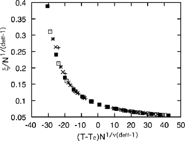
Figure 2: Scaling plot of the correlation length $(T-T_{c})N^{1/\nu(d_{eff}-1)}$-$\xi/N^{1/(d_{eff}-1)}$ is shown for $j=1.5$ and the system sizes $N=13,14,\dots,17$. The symbols $+$, $\times$, $*$, $\Box$, and $\blacksquare$ denote the system sizes of $N=13$, $14$, $15$, $16$, and $17$, respectively. The scaling parameters are set to be $1/\nu=1.36$, $d_{eff}=2.50$, and $T_{c}=5.13$; see text for details. We see that a good data collapse is achieved under a fractional value of the effective dimension $d_{eff}=2.50$.

In order to examine the validity of the scaling parameters, $d_{eff}$ and $T_{c}$, determined with the above method, we plotted, in Fig. 2, the scaled correlation length $(T-T_{c})N^{1/(\nu(d_{eff}-1))}$-$\xi/N^{1/(d_{eff}-1)}$ for $d_{eff}=2.50$, $T_{c}=5.13$, $1/\nu=1.36$, $j=1.5$, and $N=13,14,\dots,17$. These scaling parameters, namely, $d_{eff}$ and $T_{c}$, are determined from the set of system sizes $(14,16;13,16)$ via the extended finite-size-scaling analysis. (We explain how we determined $1/\nu=1.36$ afterward.) We see that the scaled data collapse into a scaling function quite satisfactorily. Hence, we confirm that the scaling parameters, $d_{eff}=2.50$ and $T_{c}=5.13$, are indeed meaningful. More significantly, we stress that our simulation data should be described under the assumption that the effective dimension takes such a fractional value.

In order to analyze the criticality further in detail, we calculated the Roomany-Wyld approximative $\beta$ function, which is given by the following formula Roomany80 ,

$$\beta_{N,N^{\prime}}(T)=\frac{1-(d_{eff}-1)\ln(\xi_{N}/\xi_{N^{\prime}})/\ln(N/N^{\prime})}{\sqrt{\partial_{T}\xi_{N}(T)\partial_{T}\xi_{N^{\prime}}(T)/\xi_{N}(T)/\xi_{N^{\prime}}(T)}}.$$ (10)

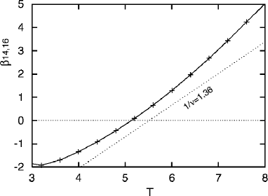
Figure 3: We plotted the beta function, $\beta_{14,16}(T)$ (10), for the same parameters as Fig. 2. From the slope at the transition point, we estimate the correlation-length critical exponent as $1/\nu=1.36$.

In Fig. 3, we plotted $\beta_{14,16}(T)$ for the same parameters as those of Fig. 2. The functional form of this $\beta$ function seems to be almost straight, indicating that the corrections to the finite-size scaling are almost negligible. This fact accounts for the good data collapse of Fig. 2 shown above. From the slope of this $\beta$ function at the transition point $T=T_{c}$, we are able to estimate the inverse of the correlation-length critical exponent as $1/\nu_{14,16}=1.36$. To summarize, we estimated the exponent $1/\nu_{N,N^{\prime}}$ from the set of system sizes $(N,N^{\prime})$. In prior to this analysis, we should determine the scaling parameters, $d_{eff}$ and $T_{c}$, from the extended finite size scaling analysis for $(N_{1},N_{2};N_{3},N_{4})$. We will exploit the $d_{eff}$-dependence of $1/\nu$ in the next subsection.

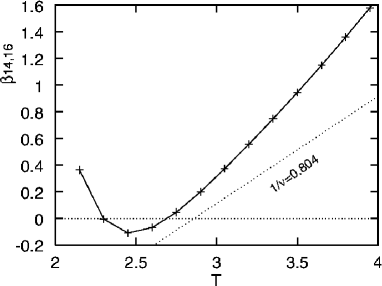
Figure 4: The beta function, $\beta_{14,16}(T)$ (10), is plotted for $j=0.9$ and $d_{eff}=2.07$. We notice that for $d_{eff}\approx 2$, the beta function gets curved, indicating that a nonstandard (essentially singular) criticality emerges. From the slope at the transition point, we estimate the correlation-length critical exponent as $1/\nu=0.804$.

Lastly, we exploit the region in close vicinity of the lower critical dimension $d=2$, at which the KT-type singularity should emerge. In Fig. 4, we present the function $\beta_{14,16}(T)$ for $j=0.9$, $T_{c}=2.74$, and $d_{eff}=2.07$; these scaling parameters were determined from the set of system sizes $(14,16;15,17)$. In contrast to the behavior shown in Fig. 3, the $\beta$ function is curved particularly in the vicinity of the transition point. Actually, we estimate the slope (critical exponent) as $1/\nu_{14,16}=0.804$ which is considerably suppressed, compared with that of Fig. 3. This feature indicates that an essentially singular-type critical behavior emerges as $d_{eff}\to 2$. For $T<T_{c}$, the $\beta$ function starts to increase, and eventually, it becomes even positive in the low-temperature regime. Such a feature may reflect an instability to the $Z_{6}$-symmetry-broken phase. Actually, it has been known Jose77 that right at $d=2$, an additional phase transition of the KT type takes place at a low temperature, where the $Z_{6}$-symmetry-breaking field becomes marginally relevant. The simulation data around this regime may be affected by the notorious logarithmic corrections to the finite-size-scaling behavior, that are inherent to the KT-type critical phenomenon.

III.2 Correlation-length critical exponent $1/\nu(d_{eff})$ for $d_{eff}$

In the above, we analyzed the criticality of the magnetic transition for $j=1.5$ and $0.9$ in terms of the effective dimension $d_{eff}$. Managing the similar analysis for various $j$, we are able to survey the $d_{eff}$-dependence of the critical exponent $1/\nu(d_{eff})$. In Fig. 5, we plotted the critical exponent $1/\nu$ for various $d_{eff}$. The exponent was determined from the set of system sizes, ($\blacksquare$) $(14,16)$, ($\times$) $(15,17)$, ($*$) $(14,16)$, and ($\Box$) $(13,17)$, for respective symbols, and the corresponding scaling parameters, namely, $d_{eff}$ and $T_{c}$, had been determined from the set of system sizes ($\blacksquare$) $(14,16;15,17)$, ($\times$) $(15,17;13,17)$, ($*$) $(14,16;13,16)$, and ($\Box$) $(15,17;13,17)$, respectively. We also plotted a result $1/\nu=1.48909(60)$ for the $d=3$ $XY$ universality class Compostrini01 with the symbol $+$. We notice that our numerical results interpolate smoothly the known limiting cases of KT ($1/\nu=0$) and $d=3$ $XY$ universality classes. As for a comparison, with a dotted line, we presented the $1/N$-expansion-approximation result up to O$(1/N)$ Ma72 ; Abe72 ; Suzuki72 ; Ferrel72 ,

$$\frac{1}{\nu}=d-2+\frac{2(3-\epsilon)(2-\epsilon)}{N(4-\epsilon)}\frac{4\sin\frac{\pi\epsilon}{2}\Gamma(2-\epsilon)}{\pi\Gamma(1-\frac{\epsilon}{2})\Gamma(2-\frac{\epsilon}{2})},$$ (11)

with $N=2$ and $\epsilon=d-2$. Rather remarkably, we see that the simulation data and the $1/N$-expansion result exhibit similar intermediate behaviors. In other words, we can make contact with such a dimensional-regularized analytical expression via the computer simulation calculation. On closer inspection, however, it seems that our first-principles simulation predicts even more convex-like functional form. Actually, our simulation result suggests a notable steep increase around $d=2$.

It is to be noted that our data extend to the regime exceeding the threshold $d=3$. As a matter of fact, we intended to cover the parameter range $2\leq d\leq 3$, when we constructed the transfer matrix in Sec. II. However, such a feature was also observed in the preceding study of the Ising ferromagnet Novotny93a . In the study, the author reported that the effective dimension does exceed the intended range, and astonishingly enough, the data are still in good agreement with the $(4-\epsilon)$-expansion result. We expect that our result makes sense even for $d_{eff}>3$ as well. Our data seem to approach to the meanfield value $1/\nu=2$ as $d\to 4$ rather directly than the $1/N$-expansion-approximation result.

In close vicinity of the lower critical dimension, particularly, around $d_{eff}\approx 2.3$, the numerical data turn out to be scattered. As noted in the preceding subsection, this data scatter should be attributed to the logarithmic corrections to the finite-size scaling, which are inherent to the KT-type critical behavior.

IV Summary and discussions

In this paper, we developed a transfer-matrix scheme to simulate the “stacked” triangular antiferromagnet embedded in $2\leq d\leq 3$. Our scheme is based on Novotny’s idea, which has been applied to the Ising ferromagnet (universality class) in $1\leq d\leq 3$ successfully Novotny92 ; Novotny93a ; Novotny93b . Here, we studied the $XY$ universality class in $2\leq d\leq 3$; the triangular antiferromagnet should belong to the $XY$ universality class due to the $Z_{6}$ symmetry Jose77 ; Tobochnik82 ; Rujan81 ; Challa86 ; Irakliotis93 . The numerical data are analyzed in terms of the extended finite-size-scaling method Novotny92 , which allows us to estimate the effective dimension $d_{eff}$. Thereby, we obtained the $d_{eff}$-dependent correlation-length critical exponent $1/\nu(d_{eff})$; see Fig. 5. We notice that our first-principles data interpolate smoothly the known limiting cases of both KT and $d=3$ $XY$ universality classes. Furthermore, we found that the intermediate behavior bears close resemblance to that of the analytical formula via the $1/N$-expansion technique. In other wards, by means of the computer simulation method, we are able to check (support) the validity of the dimensional-regularized formulas with the $\epsilon$ and $1/N$ expansion techniques. On closer inspection, our simulation result suggests a notable steep increase around $d=2$.

The present study on the stacked triangular antiferromagnet shows that the Novotny method would be generic, and it should be applicable to a wide variety of universality classes other than the Ising universality. So far, the transfer-matrix approach has been restricted to the problems in two dimensions, because it requires huge computer memory space as the system size increases. (Although the density-matrix-renormalization-group method resolves this difficulty to a considerable extent, its extension to $d=3$ is still a current topics underway Maeshima04 .) With the aid of the Novotny method, we are able to construct the transfer matrix for $d>2$ quite systematically with modest (actually, arbitrary) number of constituent spins. Moreover, we can survey the criticality even in the fractional dimensions by means of the extended finite-size-scaling analysis. This opens a way to re-examine the longstanding problems in three dimensions such as the chiral universality Kawamura98 and the Lifshitz-type multi-critical phenomenon Diehl04 .

One may wonder what affects the variation of $d_{eff}$ most significantly: Actually, there have been known two approaches in order to control $d_{eff}$ in the past studies of the Ising ferromagnet. In Ref. Novotny92 , the interaction distance $v$, in other words, the connectivity of the finite-size cluster, is tuned carefully. On the other hand, in Refs. Novotny93a ; Novotny93b , the boundary condition is twisted so as to control the thermal undulations of the magnetic domain walls. In our scheme, as explained in Sec. II, we fixed the lattice connectivity $v$, and rather varied the inter-plane interaction $j$: In this sense, we took an advantage that our system (stacked triangular antiferromagnet) is, by nature, spatially anisotropic, and so we are able to tune the inter-plane interaction freely. We suspect that our case may belong to the latter category. That is, the inter-plane interaction, somehow, controls the domain-wall undulations effectively. This interpretation is based on the fact that our system is subjected to the magnetic frustration due to the triangular antiferromagnetism, and the domain walls should be created inevitably. It is desirable that this mechanism would be exploited in the future study.

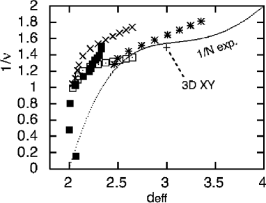
Figure 5: The inverse of the correlation-length critical exponent $1/\nu(d_{eff})$ is plotted for the effective dimension $d_{eff}$. The exponent is determined from the pair of system sizes, ($\blacksquare$) $(14,16)$ under the extended scaling analysis Novotny92 for $(14,16;15,17)$, ($\times$) $(15,17)$ with $(15,17;13,17)$, ($*$) $(14,16)$ with $(14,16;13,16)$, and ($\Box$) $(13,17)$ with $(15,17;13,17)$, for respective symbols; see text for details. We also plotted the $1/N$-expansion-approximation result up to O$(1/N)$ Ma72 ; Abe72 ; Suzuki72 ; Ferrel72 . The symbol $+$ denotes a result for the $d=3$ $XY$ model Compostrini01 .

- (1) M. A. Novotny, J. Appl. Phys. 67, 5448 (1990).
- (2) M. A. Novotny, Phys. Rev. B 46, 2939 (1992).
- (3) M. A. Novotny, Phys. Rev. Lett. 70, 109 (1993).
- (4) M A Novotny, Computer Simulation Studies in Condensed-Matter Physics IV, edited by D. P. Landau, K. K. Mon, and H.-B. Schüttler (Springer-Verlag, Berlin Heidelberg, 1993).
- (5) Y. Nishiyama, Phys. Rev. E 70, 026120 (2004).
- (6) D. P. Landau and K. Binder, Phys. Rev. B 41, 4633 (1990).
- (7) C. Ruge and F. Wagner, Phys. Rev. B 52, 4209 (1995).
- (8) D. P. Landau, Phy. Rev. B 27, 5604 (1983).
- (9) H. Kitatani and T. Oguchi, J. Phys. Soc. Jpn. 57, 1344 (1988).
- (10) S. Miyashita, H. Kitatani, and Y. Kanada, J. Phys. Soc. Jpn., 60, 1523 (1991).
- (11) S. L. A. de Queiroz and E. Domany, Phys. Rev. E 52, 4768 (1995).
- (12) S. Miyashita, J. Phys. Soc. Jpn. 66, 3411 (1997).
- (13) D. Blankschtein, M. Ma, A. N. Berker, G. S. Grest, and C. M. Soukoulis, Phys. Rev. B 29, R5250 (1984).
- (14) O. Heinonen and R. G. Petschek, Phys. Rev. B 40, 9052 (1989).
- (15) J.-J. Kim, Y. Yamada, and O. Nagai, Phys. Rev. B 41, 4760 (1990).
- (16) R. R. Netz and A. N. Berker, Phys. Rev. Lett. 66, 377 (1991).
- (17) A. Bunker, B. D. Gaulin, and C. Kallin, Phys. Rev. B 48, 15861 (1993)
- (18) B. D. Gaulin, A. Bunker, and C. Kallin, Phys. Rev. B 52, 1415 (1995).
- (19) M. L. Plumer, A. Mailhot, R. Ducharme, A. Caille, and H. T. Diep, Phys. Rev. B 47, 14312 (1993).
- (20) M. L. Plumer and A. Mailhot, Phys. Rev. B 52, 1411 (1995).
- (21) D. Dantchev and M. Krech, Phys. Rev. E 69, 046119 (2004).
- (22) J.V. José, L.P. Kadanoff, S. Kirkpatrick, and D.R. Nelson, Phys. Rev. B 16, 1217 (1977).
- (23) J. Tobochnik, Phys. Rev. B 26, 6201 (1982).
- (24) P. Ruján, G. O. Williams, H. L. Frisch, and G. Forgács, Phys. Rev. B 23, 1362 (1981).
- (25) M. S. S. Challa and D. P. Landau, Phys. Rev. B 33, 437 (1986).
- (26) P. D. Scholten and L. J. Irakliotis, Phys. Rev. B 48, 1291 (1993).
- (27) S. Ma, Phys. Rev. Lett. 29, 1311 (1972).
- (28) R. Abe, Prog. Theor. Phys., 48, 1414 (1972).
- (29) M. Suzuki, Phys. Lett. 42A, 5 (1972).
- (30) R. A. Ferrell, and D. J. Scalapino, Phys. Rev. Lett. 29, 413 (1972).
- (31) Y. Gefen, A. Aharony, Y. Shapir, and B. B. Mandelbrot, J. Phys. A: Math. Gen. 17, 435 (1984).
- (32) B. Lin and Z. R. Yang, J. Phys. A: Math. Gen. 19, L49 (1986).
- (33) Y. Taguchi, J. Phys. A: Math. Gen. 20, 6611 (1987).
- (34) U. S. M. Costa, I. Roditi, and E. M. F. Curado, J. Phys. A: Math. Gen. 20, 6001 (1987).
- (35) L. Hao and Z. R. Yang, J. Phys. A: Math. Gen. 20, 1627 (1987).
- (36) H. H. Roomany and H. W. Wyld, Phys. Rev. D 21, 3341 (1980).
- (37) M. Campostrini, M. Hasenbusch, A. Pelissetto, P. Rossi, and E. Vicari, Phys. Rev. B 63, 214503 (2001).
- (38) N. Maeshima, J. Phys. Soc. Jpn. 73, 60 (2004).
- (39) H. Kawamura, J. Phys. Condens. Matter 10, 4707 (1998).
- (40) H. W. Diehl, cond-mat/0407352.