Thermodynamic Consistency of the Dynamical Mean-Field Theory of the Double-Exchange Model

Abstract

Although diagrammatic perturbation theory fails for the dynamical-mean field theory of the double-exchange model, the theory is nevertheless $\Phi$-derivable and hence thermodynamically consistent, meaning that the same thermodynamic properties are obtained from either the partition function or the Green’s function. We verify this consistency by evaluating the magnetic susceptibility and Curie temperature for any Hund’s coupling.

The dynamical mean-field theory (DMFT) formulated in the late 1980’s by Müller-Hartmann mul:89 and Metzner and Vollhardt met:89 has developed into one of the most powerful many-body techniques for studying electronic models such as the Hubbard fre:95 ; geo:96 and double-exchange (DE) fur:95 ; mil:96 ; aus:01 ; fis:03 ; che:03 models. This theory is believed to become exact in the limit of infinite dimensions and to capture the physics of correlated electron systems even in three dimensions. Recent work on dilute magnetic semiconductors has used DMFT to study variants of the DE model cha:01 ; ara:04 with less than one local moment per site. In this paper, we reach the surprising conclusion that, unlike for the DMFT of the Hubbard model geo:96 , a diagrammatic perturbation theory containing only electronic degrees of freedom fails for the DMFT of the DE model. Nevertheless, we show that the theory remains $\Phi$-derivable in a more restrictive sense, which still implies that the partition function and Green’s function produce consistent results for thermodynamic properties such as the magnetic susceptibility and Curie temperature.

The Hamiltonian of the DE model is given by

$$H=-t\sum_{\langle i,j\rangle}\Bigl{(}c^{\dagger}_{i\alpha}c^{\,}_{j\alpha}+c^{\dagger}_{j\alpha}c^{\,}_{i\alpha}\Bigr{)}-2J_{\rm H}\sum_{i}{\bf s}_{i}\cdot{\bf S}_{i}$$ (1)

where $c^{\dagger}_{i\alpha}$ and $c_{i\alpha}$ are the creation and destruction operators for an electron with spin $\alpha$ at site $i$, ${\bf s}_{i}=(1/2)c^{\dagger}_{i\alpha}{\bf\sigma}_{\alpha\beta}c^{\,}_{i\beta}$ is the electronic spin, and ${\bf S}_{i}=S{\bf m}_{i}$ is the spin of the local moment. Repeated spin indices are summed. Within DMFT, the effective action on site 0 above $T_{\rm C}$ in zero field is given by

$$A_{\rm eff}({\bf m})=-T\sum_{n}\bar{c}_{0\alpha}(i\nu_{n})\Bigl{\{}G_{0}(i\nu_{n})^{-1}\delta_{\alpha\beta}+\tilde{J}_{\rm H}{\bf\sigma}_{\alpha\beta}\cdot{\bf m}\Bigr{\}}c_{0\beta}(i\nu_{n}),$$ (2)

where $\tilde{J}_{\rm H}=J_{\rm H}S$, $\nu_{n}=(2n+1)\pi T$, $\bar{c}_{0\alpha}(i\nu_{n})$ and $c_{0\alpha}(i\nu_{n})$ are now anticommuting Grassman variables, and $G_{0}(i\nu_{n})$ is the bare Green’s function containing dynamical information about the hopping of electrons from other sites onto site 0.

Because $A_{\rm eff}({\bf m})$ is quadratic in the Grassman variables, the full Green’s function $G(i\nu_{n})_{\alpha\beta}$ at site 0 may be readily solved by integrating over the Grassman variables, with the paramagnetic result fur:95

$$G(i\nu_{n})\underline{I}=\Bigl{\langle}\Bigl{\{}G_{0}(i\nu_{n})^{-1}\underline{I}+\tilde{J}_{\rm H}\underline{{\bf\sigma}}\cdot{\bf m}\Bigr{\}}^{-1}\Bigr{\rangle}_{{\bf m}}=\displaystyle\frac{G_{0}(i\nu_{n})^{-1}}{G_{0}(i\nu_{n})^{-2}-\tilde{J}_{\rm H}^{2}}\underline{I},$$ (3)

where $\underline{I}$ is the unity matrix in 2 x 2 spin space. The average over the orientations ${\bf m}$ of the local moment is generally given by $\langle C({\bf m})\rangle_{{\bf m}}=\int d\Omega_{{\bf m}}P({\bf m})C({\bf m})$, where $P({\bf m})\propto{\rm Tr}\Bigl{(}\exp(-A_{\rm eff}({\bf m})\Bigr{)}$ is the probability for the local moment to point in the ${\bf m}$ direction. Above $T_{\rm C}$, $P({\bf m})=1/4\pi$ is constant. Consequently, the paramagnetic self-energy is given by $\Sigma(i\nu_{n})=G_{0}(i\nu_{n})^{-1}-G(i\nu_{n})^{-1}=\tilde{J}_{\rm H}^{2}G_{0}(i\nu_{n})$. Expanded in powers of $\tilde{J}_{\rm H}$ and $G(i\nu_{n})$, we find

$$\Sigma(i\nu_{n})=-\frac{1}{2G(i\nu_{n})}+\sqrt{\displaystyle\frac{1}{4G(i\nu_{n})^{2}}+\tilde{J}_{\rm H}^{2}}=\tilde{J}_{\rm H}^{2}G(i\nu_{n})-\tilde{J}_{\rm H}^{4}G(i\nu_{n})^{3}+2\tilde{J}_{\rm H}^{6}G(i\nu_{n})^{5}+\ldots.$$ (4)

On a Bethe lattice, these relations are closed by the analytic expression fur:95 ; geo:96

$$\underline{G}_{0}(i\nu_{n})^{-1}=z_{n}\underline{I}-\frac{W^{2}}{16}\underline{G}(i\nu_{n}),$$ (5)

where $z_{n}=i\nu_{n}+\mu$ and $W$ is the full bandwidth of the non-interacting, semicircular density-of-states. We denote the full spin dependence for later use.

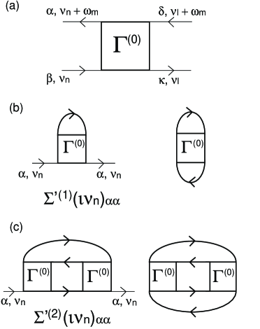
Figure 1: (a) The bare vertex function; (b) and (c) Compact diagrams that contribute to $\Phi$ for the electronic effective action $A_{\rm eff}^{\prime}$ on the right with their associated self-energies on the left.

Diagrammatic perturbation theory is customarily formulated in terms of the bare vertex function $\Gamma^{(0)}(l,n;m)^{\beta\alpha;\delta\kappa}$ sketched in Fig.1(a) with $\omega_{m}=2m\pi T$. The bare vertex function may be associated with the two-particle interaction in the purely electronic effective action abr:63

$$A_{\rm eff}^{\prime}=-T\displaystyle\sum_{n}\bar{c}_{0\alpha}(i\nu_{n})G_{0}(i\nu_{n})^{-1}c_{0\alpha}(i\nu_{n})$$

$$-\displaystyle\frac{T^{3}}{4}\displaystyle\sum_{l,n,m}\bar{c}_{0\alpha}(i\nu_{n}+i\omega_{m})c_{0\beta}(i\nu_{n})\Gamma^{(0)}(l,n;m)^{\beta\alpha;\delta\kappa}\bar{c}_{0\kappa}(i\nu_{l})c_{0\delta}(i\nu_{l}+i\omega_{m}).$$ (6)

Hence, the bare vertex function must satisfy the crossing symmetries $\Gamma^{(0)}(l,l+m;n-l)^{\delta\alpha;\beta\kappa}=\Gamma^{(0)}(n+m,n;l-n)^{\beta\kappa;\delta\alpha}=-\Gamma^{(0)}(l,n;m)^{\beta\alpha;\delta\kappa}$. There are two ways to calculate $\Gamma^{(0)}(l,n;m)^{\beta\alpha;\delta\kappa}$. First, we can take the $J_{\rm H}\rightarrow 0$ limit of the full irreducible vertex $\Gamma(l,n;m)^{\beta\alpha;\delta\kappa}$ obtained from the Bethe-Salpeter equation for the magnetic susceptibility fis:03 ; fis:un . Alternatively, we can associate the lowest-order, $J_{\rm H}^{2}$ contribution to the partition function $Z=\langle{\rm Tr}\Bigl{(}\exp(-A_{\rm eff}({\bf m}))\Bigr{)}\rangle_{{\bf m}}$ with the contribution to the partition function $Z^{\prime}={\rm Tr}\Bigl{(}\exp(-A_{\rm eff}^{\prime})\Bigr{)}$, sketched as the compact diagram in Fig.1(b) (with internal lines given by the bare Green’s functions $G_{0}(i\nu_{n})_{\alpha\beta}$). Both methods yield the same result:

$$\Gamma^{(0)}(l,n;m)^{\beta\alpha;\delta\kappa}=\frac{1}{3}\beta\tilde{J}_{\rm H}^{2}\Bigl{\{}{\bf\sigma}_{\beta\alpha}\cdot{\bf\sigma}_{\delta\kappa}\delta_{m,0}-{\bf\sigma}_{\delta\alpha}\cdot{\bf\sigma}_{\beta\kappa}\delta_{ln}\Bigr{\}},$$ (7)

which satisfies the crossing symmetries.

However, replacing $A_{\rm eff}({\bf m})$ by $A_{\rm eff}^{\prime}$ produces an inequivalent theory ineq . For example, expanding $Z$ and $Z^{\prime}$ in powers of $J_{\rm H}$ yields the results

$$Z=Z_{0}\Bigl{\{}1-\tilde{J}_{\rm H}^{2}\sum_{n}G_{0}(i\nu_{n})^{2}+\frac{1}{2}\tilde{J}_{\rm H}^{4}\sum_{l\neq n}G_{0}(i\nu_{l})^{2}G_{0}(i\nu_{n})^{2}+{\cal O}(\tilde{J}_{\rm H}^{6})\Bigr{\}},$$ (8)

$$Z^{\prime}=Z_{0}\Bigl{\{}1-\tilde{J}_{\rm H}^{2}\sum_{n}G_{0}(i\nu_{n})^{2}+\frac{5}{6}\tilde{J}_{\rm H}^{4}\sum_{l\neq n}G_{0}(i\nu_{l})^{2}G_{0}(i\nu_{n})^{2}+{\cal O}(\tilde{J}_{\rm H}^{6})\Bigr{\}},$$ (9)

which disagree to order $\tilde{J}_{\rm H}^{4}$. Hence, it is not possible by averaging over the local moments to reduce the Hund’s coupling to an effective two-particle interaction. In other words, the Hund’s coupling produces fourth and higher-order electronic interactions that require higher-order vertex functions in the electronic action.

A theory is usually said to be $\Phi$-derivable if a functional $\Phi(\{\underline{G}(i\nu_{n})\})$, constructed from the sum of compact diagrams in terms of the full Green’s functions and the bare vertex functions, can be found to satisfy the condition $\Sigma(i\nu_{n})_{\alpha\beta}=\delta\Phi/\delta G(i\nu_{n})_{\alpha\beta}$. As discussed by Baym bay:62 , a $\Phi$-derivable theory may readily be shown to be thermodynamically consistent, meaning that thermodynamic properties can be evaluated either from the Green’s function or from the partition function $Z$. For a $\Phi$-derivable theory, the partition function $Z$ or free energy $-T\log Z$ may be constructed in terms of $\Phi$ from the relation

$$-\log Z=\Phi-\sum_{n}{\rm Tr}\Bigl{\{}\underline{\Sigma}(i\nu_{n})\underline{G}(i\nu_{n})\Bigr{\}}+\sum_{n}{\rm Tr}\log\Bigl{\{}\underline{G}(i\nu_{n})\Bigr{\}},$$ (10)

which is stationary under variations of $\underline{G}(i\nu_{n})$. Whereas Baym’s original work was intended for systems of interacting Fermions and Bosons, the notion of $\Phi$-derivability has been extended to systems of interacting electrons and spins bic:87 and to disordered alloys lea:68 .

From the discussion above, it is clear that even if it exists, $\Phi$ cannot be constructed in terms of the bare vertex functions. When the action contains only two-particle interactions such as for the Hubbard model, then the first two terms in $\Phi$ are represented by the compact diagrams on the right-hand side of Figs.1(b) and (c) with the corresponding self-energies $\Sigma(i\nu_{n})_{\alpha\alpha}=\delta\Phi/\delta G(i\nu_{n})_{\alpha\alpha}$ sketched on the left-hand side. Not surprisingly, substituting our earlier expression for the bare vertex function produces the correct first-order self-energy $\Sigma^{{}^{\prime}(1)}(i\nu_{n})=\tilde{J}_{\rm H}^{2}G(i\nu_{n})$ but the wrong second-order self-energy $\Sigma^{{}^{\prime}(2)}(i\nu_{n})=-(\tilde{J}_{\rm H}^{4}/3)\Bigl{\{}2G(i\nu_{n})\sum_{l}G(i\nu_{l})^{2}+G(i\nu_{n})^{3}\Bigr{\}}$. Notice from Eq.(4) that the correct second-order self-energy $\Sigma^{(2)}(i\nu_{n})=-\tilde{J}_{\rm H}^{4}G(i\nu_{n})^{3}$ does not involve a Matsubara summation. Hence, the DMFT of the DE model is not $\Phi$-derivable in the strict diagrammatic sense stated above.

Despite the failure of a diagrammatic expansion in powers of $\underline{\Gamma}^{(0)}$, a functional $\Phi(\{\underline{G}(i\nu_{n})\})$ can still be constructed to satisfy the condition $\Sigma(i\nu_{n})_{\alpha\alpha}=\delta\Phi/\delta G(i\nu_{n})_{\alpha\alpha}$. Starting from Eq.(3) and Dyson’s equation for the self-energy, we find that $\delta\Sigma(i\nu_{l})_{\alpha\alpha}/\delta G(i\nu_{n})_{\beta\beta}=(\underline{K}^{-1})_{ln}^{\alpha\beta}+\delta_{ln}\delta_{\alpha\beta}G(i\nu_{n})^{-2}$, where $\underline{K}$ is the Jacobian

$$K^{\alpha\beta}_{ln}=\displaystyle\frac{\delta G(i\nu_{n})_{\beta\beta}}{\delta[G_{0}(i\nu_{l})_{\alpha\alpha}]^{-1}}=-\delta_{ln}\displaystyle\frac{1}{a_{n}^{2}}\Biggl{\{}\displaystyle\frac{2\tilde{J}_{\rm H}^{2}}{3}+b_{n}\delta_{\alpha\beta}\Biggr{\}}+\displaystyle\frac{\tilde{J}_{\rm H}^{2}}{3a_{l}a_{n}}\Bigl{(}2\delta_{\alpha\beta}-1\Bigr{)},$$ (11)

with $a_{n}=G_{0}(i\nu_{n})^{-2}-\tilde{J}_{\rm H}^{2}$ and $b_{n}=G_{0}(i\nu_{n})^{-2}-\tilde{J}_{\rm H}^{2}/3$. This Jacobian can be inverted with the general result

$$\frac{\delta\Sigma(i\nu_{l})_{\alpha\alpha}}{\delta G(i\nu_{n})_{\beta\beta}}=-\delta_{ln}\displaystyle\frac{\tilde{J}_{\rm H}^{2}a_{n}^{2}}{3b_{n}}\Biggl{\{}\displaystyle\frac{2}{2a_{n}-3b_{n}}+\delta_{\alpha\beta}G_{0}(i\nu_{n})^{2}\Biggr{\}}-\displaystyle\frac{\tilde{J}_{\rm H}^{2}}{3-2\tilde{J}_{\rm H}^{2}\sum_{r}1/b_{r}}\displaystyle\frac{a_{l}a_{n}}{b_{l}b_{n}}\Bigl{(}2\delta_{\alpha\beta}-1\Bigr{)}.$$ (12)

It can be shown fis:un that the right-hand side equals $-T\,\Gamma(l,n;m=0)^{\alpha\alpha;\beta\beta}$ where $\Gamma(l,n;m)^{\beta\alpha;\delta\kappa}$ is the full irreducible vertex of the Bethe-Salpeter equation. The functional $\Phi$ must exist because the curl of the self-energy vanishes: $\delta\Sigma(i\nu_{n})_{\alpha\alpha}/\delta G(i\nu_{l})_{\beta\beta}-\delta\Sigma(i\nu_{l})_{\beta\beta}/\delta G(i\nu_{n})_{\alpha\alpha}=0$.

By construction, $\Phi^{(1)}$ (second order in $J_{\rm H}$) is represented by the compact diagram in Fig.1(b) and is given in terms of the bare vertex function by

$$\Phi^{(1)} =-\displaystyle\frac{T}{2}\sum_{l,r}\Gamma^{(0)}(l,r;0)^{\alpha\alpha;\beta\beta}G(i\nu_{l})_{\alpha\alpha}G(i\nu_{r})_{\beta\beta}=-\displaystyle\frac{\tilde{J}_{\rm H}^{2}}{6}\biggl{\{}\displaystyle\sum_{l,n}G(i\nu_{l})_{\alpha\alpha}$$ (13)

$$\times\Bigl{(}G(i\nu_{n})_{\alpha\alpha}-G(i\nu_{n})_{\bar{\alpha}\bar{\alpha}}\Bigr{)}-\displaystyle\sum_{n}G(i\nu_{n})_{\alpha\alpha}^{2}-2\displaystyle\sum_{n}G(i\nu_{n})_{\alpha\alpha}G(i\nu_{n})_{\bar{\alpha}\bar{\alpha}}\biggr{\}},$$

where $\bar{\alpha}$ is the opposite spin to $\alpha$. After expanding and integrating Eq.(12) rcurv , we find that $\Phi^{(2)}$ (fourth order in $J_{\rm H}$) is given by

$$\Phi^{(2)} =\displaystyle\frac{\tilde{J}_{\rm H}^{4}}{9}\biggl{\{}-\displaystyle\frac{1}{4}\displaystyle\sum_{n}G(i\nu_{n})_{\alpha\alpha}^{4}-2\displaystyle\sum_{n}G(i\nu_{n})_{\alpha\alpha}^{2}G(i\nu_{n})_{\bar{\alpha}\bar{\alpha}}^{2}-\displaystyle\sum_{l,n,r}G(i\nu_{r})_{\alpha\alpha}G(i\nu_{r})_{\bar{\alpha}\bar{\alpha}}G(i\nu_{l})_{\alpha\alpha}$$ (14)

$$\times\Bigl{(}G(i\nu_{n})_{\alpha\alpha}-G(i\nu_{n})_{\bar{\alpha}\bar{\alpha}}\Bigr{)}+\displaystyle\frac{2}{3}\displaystyle\sum_{l,n}G(i\nu_{n})_{\alpha\alpha}^{3}\Bigl{(}G(i\nu_{l})_{\alpha\alpha}-G(i\nu_{l})_{\bar{\alpha}\bar{\alpha}}\Bigr{)}\biggr{\}}.$$

Unlike $\Phi^{(1)}$, $\Phi^{(2)}$ cannot be represented by a compact diagram involving only the bare vertex functions. So far, all of our results are valid for any lattice topology.

We have verified the thermodynamic consistency of the DMFT by calculating the magnetic susceptibility from both the Green’s function and the partition function. With a magnetic field ${\bf H}=H{\bf z}$ coupled to both the local moments and the electrons, the effective action becomes

$$A_{\rm eff}({\bf m})=-T\sum_{n}\bar{c}_{0\alpha}(i\nu_{n})\Bigl{\{}G_{0}(i\nu_{n})^{-1}_{\alpha\beta}+\Bigl{(}\tilde{J}_{\rm H}{\bf m}+\frac{1}{2}H{\bf z}\Bigr{)}\cdot{\bf\sigma}_{\alpha\beta}\Bigr{\}}c_{0\beta}(i\nu_{n})-\beta HSm_{z}.$$ (15)

Parameterizing the bare inverse Green’s function as $\underline{G}_{0}(i\nu_{n})^{-1}=(z_{n}+R_{n})\underline{I}+Q_{n}\underline{\sigma}_{z}$ and using Eq.(5) for the full Green’s function, we solve for $R_{n}$ and $Q_{n}$ on a Bethe lattice from the expression

$$R_{n}\underline{I}+Q_{n}\underline{\sigma}_{z}=-\frac{W^{2}}{16}\Bigl{\langle}\Bigl{\{}(z_{n}+R_{n})\underline{I}+\Bigl{(}\tilde{J}_{\rm H}{\bf m}+(Q_{n}+H/2){\bf z}\Bigr{)}\cdot\underline{{\bf\sigma}}\Bigr{\}}^{-1}\Bigr{\rangle}_{{\bf m}}.$$ (16)

To linear order in the field, $R_{n}$ and $Q_{n}$ satisfy the implicit relations

$$R_{n}=-\frac{W^{2}}{16}\frac{z_{n}+R_{n}}{(z_{n}+R_{n})^{2}-\tilde{J}_{\rm H}^{2}},$$ (17)

$$Q_{n}=\frac{H(z_{n}+R_{n})-2\tilde{J}_{\rm H}M_{lm}R_{n}}{2(z_{n}+2R_{n})U_{n}}-\frac{H}{2},$$ (18)

where

$$U_{n}=1-\frac{32\tilde{J}_{\rm H}^{2}}{3W^{2}}\frac{R_{n}^{2}}{(z_{n}+R_{n})(z_{n}+2R_{n})}.$$ (19)

After integrating $\exp(-A_{\rm eff}({\bf m}))$ over the Grassman variables, we find that the probability for the local moment to point along ${\bf m}$ is

$$P({\bf m})\propto\exp\Biggl{\{}\sum_{n}\log\Biggl{(}1-\frac{\tilde{J}_{\rm H}(2Q_{n}+H)m_{z}}{(z_{n}+R_{n})^{2}-\tilde{J}_{\rm H}^{2}}\Biggr{)}+\beta HSm_{z}\Biggr{\}}\propto\exp(\beta J_{eff}M_{lm}m_{z}),$$ (20)

where the local-moment order parameter $M_{lm}=\langle m_{z}\rangle$ is solved from the condition $M_{lm}=J_{eff}M_{lm}\beta/3$. The electronic order parameter $M_{el}=2\langle s_{0z}\rangle$ is obtained from the summation $M_{el}=-(32T/W^{2})\sum_{n}Q_{n}$. The total susceptibility is then given by the zero-field limit of $\chi=(SM_{lm}+M_{el}/2)/H$. To calculate the susceptibility from the partition function, we first expand $Z$ to second order in $H$ and $M_{lm}$ and then use $\chi=(T/H)\partial\log Z/\partial H|_{H=0}$. The latter technique is formally equivalent to evaluating the susceptibility from the Bethe-Salpeter equation fis:03 .

These two sets of calculations do indeed produce the same magnetic susceptibility, which may be written as

$$\chi=\frac{1}{3T}\frac{S_{\rm eff}(T)^{2}}{1-(\tilde{J}_{\rm H}/W)^{2}G_{1}(T)}+\frac{3T}{4W^{2}}\Bigl{(}G_{1}(T)-G_{2}(T)\Bigr{)}+\frac{8\tilde{J}_{\rm H}^{2}T}{W^{4}}G_{1}(T),$$ (21)

$$S_{\rm eff}(T)=S+\frac{3\tilde{J}_{\rm H}T}{2W^{2}}\Bigl{(}G_{1}(T)-G_{2}(T)\Bigr{)},$$ (22)

where the functions $G_{1}(T)$ and $G_{2}(T)$ are formally given by the Matsubara sums

$$G_{1}(T)=-\frac{32}{3}\sum_{n}\frac{R_{n}^{2}}{(z_{n}+R_{n})(z_{n}+2R_{n})U_{n}},$$ (23)

$$G_{2}(T)=-\frac{32}{3}\sum_{n}\frac{R_{n}}{(z_{n}+R_{n})U_{n}}.$$ (24)

The Curie temperature $T_{\rm C}$ is solved from the condition $G_{1}(T_{C})=(W/\tilde{J}_{\rm H})^{2}$.

Previous results fis:03 in the $J_{\rm H}\rightarrow\infty$ limit are reproduced limit by taking $\mu={\rm sgn}(p-1)\tilde{J}_{\rm H}+\delta\mu$ where $|\delta\mu|\leq W/(2\sqrt{2})$ and $p$ is the electron filling ($p=1$ means one electron per site). The general expression for the magnetic susceptibility shall be studied in a future publication. We pause here to note that the effective spin $S_{\rm eff}(T)$ may be either larger or smaller than $S$ depending on the sign of the Hund’s coupling $J_{\rm H}$. The temperature dependence of $S_{\rm eff}(T)$ and the deviation of $1-(\tilde{J}_{\rm H}/W)^{2}G_{1}(T)$ from $T-T_{\rm C}$ are both caused by electronic correlations that are absent in a local-moment system fis:03 . The second and third sets of terms in Eq.(21) correspond to the Pauli susceptibility of the electrons.

Although $\Phi(\{\underline{G}(i\nu_{n})\})$ has no simple diagrammatic interpretation, the existence of this functional means that we may still use Eq.(10) to establish the thermodynamic consistency of the DMFT of the DE model. Diagrammatics may be recovered for a more sophisticated model where the classical local moments are replaced by fully quantum-mechanical operators and we introduce an additional propagator corresponding to those local spins. It may also be possible to develop a more complex diagrammatics for classical local spins in terms of higher-order vertex functions.

Finally, we note that whereas any conserving theory (in the sense of Baym and Kadanoff bay:62 ) is thermodynamically consistent, it is not true that all thermodynamically consistent theories are conserving. Indeed, that is the case here since the DMFT violates the Ward identities associated with charge and spin conservation.

It is a pleasure to acknowledge helpful conversations with Dr. Gonzalo Alvarez and Prof. Jim Freericks. This research was sponsored by the U.S. Department of Energy under contract DE-AC05-00OR22725 with Oak Ridge National Laboratory, managed by UT-Battelle, LLC and by the National Science Foundation under Grant No. EPS-0132289 (ND EPSCoR) and DMR-0312680.

References

• (1) E. Müller-Hartmann, Z. Phys. B 74, 507 (1989); ibid. 76, 211 (1989).
• (2) W. Metzner and D. Vollhardt, Phys. Rev. Lett. 62, 324 (1989).
• (3) J.K. Freericks and M. Jarrell, Phys. Rev. Lett. 74, 186 (1995).
• (4) Applications of DMFT to the Hubbard model and additional references are contained in the comprehensive review article: A. Georges, G. Kotliar, W. Krauth, and M.J. Rozenberg, Rev. Mod. Phys. 68, 13 (1996).
• (5) N. Furukawa, J. Phys. Soc. Jpn. 64, 2754 (1995); ibid. 64, 3164 (1995).
• (6) A.J. Millis, R. Mueller, and B.I. Shraiman, Phys. Rev. B 54, 5389 (1996); ibid. 54, 5405 (1996); B. Michaelis and A.J. Millis, Phys. Rev. B 68, 115111 (2003).
• (7) M. Auslender and E. Kogan, Phys. Rev. B 65, 012408 (2001); Europhys. Lett. 59, 277 (2002).
• (8) R.S. Fishman and M. Jarrell, J. Appl. Phys. 93, 7148 (2003); Phys. Rev. B 67, 100403 (2003).
• (9) A. Chernyshev and R.S. Fishman, Phys. Rev. Lett. 90, 177202 (2003).
• (10) A. Chattopadhyay, S. Das Sarma, and A.J. Millis, Phys. Rev. Lett. 87, 227202 (2001).
• (11) K. Arayanpour, J. Moreno, M. Jarrell, and R.S. Fishman, cond-mat 0402289.
• (12) For a general reference, see A.A. Abrikosov, L.P. Gorkov, and I.E. Dzyaloshinski, Methods of Quantum Field Theory in Statistical Mechanics (Englewood Cliffs, Prentice Hall, 1963).
• (13) R.S. Fishman and M. Jarrell, unpublished.
• (14) The electronic effective action $A_{\rm eff}^{\prime}$ would still produce an inequivalent theory even if the three-dimensional local spins $S{\bf m}$ were replaced by Ising spins $\pm S{\bf z}$.
• (15) G. Baym and L.P. Kadanoff, Phys. Rev. 124, 287 (1961); G. Baym, Phys. Rev. 127, 1391 (1962).
• (16) N.E. Bickers, Rev. Mod. Phys. 59, 845 (1987).
• (17) P.L. Leath, Phys. Rev. 171, 725 (1968).
• (18) Due to the term containing $\Bigl{\{}1-(2/3)\tilde{J}_{\rm H}^{2}\sum_{l}\Bigl{(}G_{0}(i\nu_{l})^{-2}-\tilde{J}_{\rm H}^{2}/3\Bigr{)}^{-1}\Bigr{\}}^{-1}$ in the irreducible vertex function $\underline{\Gamma}$, the radius of convergence of the expansion in powers of $\tilde{J}_{\rm H}$ is of order $T$. In the limit $J_{\rm H}\rightarrow\infty$, $\underline{\Gamma}$ depends on the cutoff $n_{\chi}$ of the Matsubara sum fis:03 .
• (19) In the $J_{\rm H}\rightarrow\infty$ limit, $G_{1}(T)\rightarrow(W/\tilde{J}_{\rm H})^{2}F_{1}(T)$ and $G_{2}(T)\rightarrow(W^{2}/3\tilde{J}_{\rm H}T)\bigl{\{}|p-1|-1-2\,{\rm sgn}(p-1)F_{2}(T)\bigr{\}}$, where $F_{1}(T)$ and $F_{2}(T)$ were defined in Ref.fis:03 .