Symmetry breaking in the self-consistent Kohn-Sham equations

Abstract

The Kohn-Sham (KS) equations determine, in a self-consistent way, the particle density of an interacting fermion system at thermal equilibrium. We consider a situation when the KS equations are known to have a unique solution at high temperatures and that this solution is a uniform particle density. We prove that, at zero temperature, there are stable solutions that are not uniform. We provide the general principles behind this phenomenon, namely the conditions when it can be observed and how to construct these non-uniform solutions. Two concrete examples are provided, including fermions on the sphere which are shown to crystallize in a structure that resembles the C₆₀ molecule.

1 Introduction

We consider a system of $N$ interacting fermions in a finite volume. Since we want to avoid the surface effects, we actually consider the fermions moving on toruses and spheres, or, more generally, on a closed Riemann manifold ${\cal M}$ of finite volume $\Omega$. According to the Kohn-Sham theory [1] (and later extensions [2]), the particle density at thermal equilibrium at a temperature $T$ ($\beta=1/kT$) is a solution of the following set of equations:

$$(H_{0}+V_{n})\phi_{i}=\epsilon_{i}\phi_{i}$$ (1)

$$n(x)=\sum_{i}\left(1+e^{\beta(\epsilon_{i}-\mu)}\right)^{-1}|\phi_{i}(x)|^{2},$$ (2)

with $V_{n}$ an effective potential depending entirely on the particle density $n$ and $\mu$ determined from $\int n(x)dx=N$. $H_{0}$ is the single particle, non-interacting Hamiltonian. We refer to

$$H_{n}\equiv H_{0}+\lambda V_{n}$$ (3)

as the Kohn-Sham Hamiltonian, where we introduced the coupling constant $\lambda$ for convenience. We will neglect the spin degree of freedom.

There is no closed form of $V_{n}$. However, at least for the electron gas, there is a set of very successful, explicit approximations, which already provide numerical results that are within the so called ”chemical precision” [3]. Although in this paper we do not use a specific approximation, we will often make reference to two such approximations in order to check our assumptions. They are the Local Density Approximation (LDA): $V_{n}=v*n+v_{xc}(n)$ ($v$ the two body interaction), i.e. $V_{n}$ is the sum between the Hartree potential and a function of density, and the quadratic approximation (QA): $V_{n}=K*n$, i.e. $V_{n}$ is the convolution of the density with a certain kernel. The mathematical structure of QA is the same as that of the Hartree approximation.

In this paper, we are not concerned with the physical and mathematical principles leading to the KS equations, but rather with the mathematical structure of these equations, in particular with the question of uniqueness at zero temperature. In other words, we have already assumed $v$-representability, picked our approximation for $V_{n}$ and we are ready to compute the self-consistent solutions. What should we expect? Well, as already demonstrated (see for example Ref. [4]), even for local approximations, we should expect a very rich structure, which may include multiple solutions, symmetry breaking etc.. While previous studies used purely numerical methods, here we use group theoretical methods and functional analysis to study this structure.

Let us discuss first what it is known about the KS equations at finite temperature and finite volume. The notation $\|\phi\|_{L^{p}}$ stands for $[\int_{\cal M}|\phi(x)|^{p}dx]^{1/p}$ and $\phi\in L^{p}$ means $\|\phi\|_{L^{p}}<\infty$. Assume the following:

A1)

$H_{0}$ is self adjoint, bounded from below; for $-a$ below its energy spectrum, the kernel $(H_{0}+a)^{-2}(x,x^{\prime})$ is continuous (with respect to $x$ and $x^{\prime}$) and

$$k_{a}\equiv\sup_{x\in{\cal M}}(H_{0}+a)^{-2}(x,x)<\infty.$$ (4)

A2)

$V_{n}\in L^{2}({\cal M})$ and $w\equiv\sup\|V_{n}\|_{L^{2}}<\infty$, where the supremum is taken over all $n$ in

$$S^{N}\equiv\{n\in L^{1}({\cal M}),\ \|n\|_{L^{1}}=N\}.$$ (5)

As $H_{0}$ is in general equal to minus the Laplace operator, A1 is easy to check for 1, 2 and 3 dimensional toruses or spheres. It fails in 4 and higher dimensions. Since ${\cal M}$ is of finite volume, A1 automatically implies that $\exp(-\beta H_{0})$ is trace class. A1 also implies that $\|f\|_{L^{\infty}}\leq\sqrt{k_{a}}\|(H_{0}+a)f\|_{L^{2}}$. Together with A2 (easy to verify for LDA and QA [5, 6]), this leads to

$$\|V_{n}(H_{0}+a)^{-1}\|\leq w\sqrt{k_{a}}\equiv\gamma_{a}.$$ (6)

Then, $H_{n}$ is self-adjoint for all $n\in S^{N}$ and, as it follows from Ref. [5], the Kohn-Sham equations can be formulated as a fixed point problem:

Theorem 1. For $T>0$, the following map is well defined:

$$\textsf{T}:S^{N}\rightarrow S^{N}$$

$$S^{N}\ni n\rightarrow\textsf{T}[n](x)=\left(1+e^{\beta(H_{n}-\mu)}\right)^{-1}(x,x),$$ (7)

where $\mu$ is the unique solution of $N=Tr\left(1+e^{\beta(H_{n}-\mu)}\right)^{-1}$. The fixed points of T generate all possible solutions of the KS equations.

Many will recognize in Eq. (1) the usual formulation of the KS problem in terms of the density matrix. When appealing to the fixed point theorem, the functional form of the map T and its domain of definition are equally important. What is new in the above result is that T is well defined for all densities which integrate to $N$.

Apart from complications that may occur at low particle densities and which will not be addressed here, the following assumption can be easily verified for LDA and QA (see Ref. [5, 6]):

A3)

There exists $\chi<\infty$ such that

$$\|V_{n}-V_{n^{\prime}}\|_{L^{1}}\leq\chi\|n-n^{\prime}\|_{L^{1}},$$ (8)

for any $n$, $n^{\prime}\in S^{N}$.

If A1-A3 are satisfied, then there exists $\kappa$, which is a function of $\lambda$, such that [5]

$$\|\textsf{T}[n]-\textsf{T}[n^{\prime}]\|_{L^{1}}\leq\kappa\|n-n^{\prime}\|_{L^{1}},$$ (9)

on the entire $S^{N}$. For $\lambda$ smaller than a critical value $\lambda_{c}$, T becomes a contraction and, consequently, it has a unique fixed point. If the constants can be chosen independent of temperature in A1-A3, it is not hard to show that $\lambda_{c}$ increases with temperature. In other words, if $\lambda$ is kept fixed, A1-A3 (and the fact that $\Omega$ is finite) guaranties the existence of a unique fixed point of T at high temperatures.

Let us end the finite temperature case with a few remarks. For an exact $V_{n}$, the existence and uniqueness, at any finite $T$, will follow from the convexity of the functional [7], provided that the equilibrium density can be written as in Eq. (2) (i.e. is $v$-representable). In practice, we don’t have the exact $V_{n}$ and $v$-representability has not been yet proved or disproved. Also, in the thermodynamic limit, where systems can have multiple coexisting phases, the issue of uniqueness becomes more delicate and definitely there are many opened questions here. Thus, the question of existence and uniqueness in the finite temperature Kohn-Sham equations is not trivial.

The situation at zero temperature is more delicate. The density now becomes $n(x)=\sum|\phi_{i}(x)|^{2}$ where the sum goes over the lowest $N$ energy states of $H_{n}$. If the last occupied energy level is degenerate and only partially occupied, there is an ambiguity in defining $n(x)$. In this paper, we deal exactly with this situation.

Let us assume that that there is a continuous group $G_{c}$ acting ergodically on ${\cal M}$ and preserving the Riemann structure. On torus or sphere, this group will be simply the translations or rotations. Let us consider the natural unitary representation of $G_{c}$ in $L^{2}({\cal M})$:

$$G_{c}\ni g\rightarrow\hat{g},\ (\hat{g}f)(x)=f(gx).$$ (10)

We assume that $H_{0}$ commutes with all $\hat{g}$ and that every symmetry of the particle density is automatically a symmetry of the effective potential:

A4)

If $n(gx)=n(x)$, then $V_{n}(gx)=V_{n}(x)$ (equivalently $\hat{g}V_{n}\hat{g}^{-1}=V_{n}$).

This assumption can be easily verified for LDA and QA. Besides other things, A4 implies that $V_{n}$ is a constant if $n(x)$ is uniform, and we can fix this constant to zero. In other words, the Kohn-Sham Hamiltonian reduces to $H_{0}$ if $n(x)=\bar{n}$ ($\bar{n}=N/\Omega$). Then, it is trivial to show that, at any finite temperature, $\bar{n}$ is a solution of the KS equations. With our assumptions, we also know that this is the only solution at high temperatures. At zero temperature, assume that, if we populate with $N$ particles the energy levels of $H_{0}$, from smaller to higher energies, we end up with $N_{0}$ particles on the last occupied energy level, assumed $d$-fold degenerate with $d>N_{0}$. We refer to this level and its energy as the Fermi level and Fermi energy $\epsilon_{F}^{0}$. If we can find $N_{0}$ states at the Fermi level so as to generate a uniform particle density, then $\bar{n}$ is a solution of the KS equations. If there is no such combination of states, than either there is no solution, the solution is not uniform or we need to consider fractional occupation numbers. We will not discuss here the last possibility, but rather concentrate to the $T\rightarrow 0$ limit of Eqs. (1) and (2).

We now show when and how the non-uniform solutions can be found. We look for a finite subgroup $G$ of $G_{c}$, which has to satisfy two simple conditions. We index its irreducible representations by $\Gamma$ and use the symbol $|\Gamma|$ to specify their dimension. Let $P_{\Gamma}$ denote the projectors

$$P_{\Gamma}=\frac{|\Gamma|}{|G|}\sum\limits_{g\in G}\chi_{\Gamma}(g)\hat{g},$$ (11)

with the following properties

$$P_{\Gamma}P_{\Gamma\prime}=\delta_{\Gamma\Gamma\prime},\ \ \sum_{\Gamma}P_{\Gamma}=I.$$ (12)

Above, $|G|$ denotes the cardinal of $G$ and $\chi_{\Gamma}(g)$ the character of $g$ in the representation $\Gamma$. Let ${\cal H}_{F}$ denote the eigenspace of $H_{0}$ corresponding to $\epsilon_{F}^{0}$. This space is invariant to $G_{c}$ and it decomposes according to the irreducible representations of $G$: ${\cal H}_{F}=\oplus_{i}P_{\Gamma_{i}}{\cal H}_{F}$. The sum goes only over those $\Gamma$ for which $P_{\Gamma}{\cal H}_{F}\neq 0$. In general, $\dim P_{\Gamma_{i}}{\cal H}_{F}=n_{i}|\Gamma_{i}|$, where $n_{i}$ is the number of representations $\Gamma_{i}$ on ${\cal H}_{F}$. The subgroup $G$ we look for must satisfy the following:

A5)

$\dim P_{\Gamma_{i}}{\cal H}_{F}=|\Gamma_{i}|$, i.e. we have irreducible representations of $G$ in each $P_{\Gamma_{i}}{\cal H}_{F}$.

A6)

$|\Gamma_{i}|=N_{0}$ for some $i$ (we rearrange so that $i=0$).

Let now $n_{0}(x)$ be the particle density when we populate all the states of $H_{0}$ below $\epsilon_{F}^{0}$ plus the $N_{0}$ states in $P_{\Gamma_{0}}{\cal H}_{F}$. Since we assumed that $\dim{\cal H}_{F}>N_{0}$, $n_{0}(x)$ is not uniform. The last condition is on the effective potential:

A7)

If $V_{\Gamma_{i}}\equiv\langle\phi^{0}_{\Gamma_{i}},V_{n_{0}}\phi^{0}_{\Gamma_{i}}\rangle$ with $\phi^{0}_{\Gamma_{i}}$ any norm one vector from $P_{\Gamma_{i}}{\cal H}_{F}$, then

$$V_{\Gamma_{i}}-V_{\Gamma_{0}}>0,\textrm{for all}\ i>0.$$ (13)

If the subgroup $G$ satisfying A5-A6 exists and the effective potential satisfies A7, then, at least for small $\lambda$, the zero temperature KS equations have a non-uniform solution,

$$n(x)=n_{0}(x)+o(\lambda).$$ (14)

This is our main result.

We end our long introduction with a discussion of the conditions A5-A7. The assumption A5 greatly simplifies our proof, but it is not essential (though we don’t have a proof without A5). A6 assures the closed shell condition and is essential. It can be relaxed, for example, we can have two completely filled shells. However, we believe that, in the ground state configuration, all $N_{0}$ particles occupied the same (lowest) energy level.

Condition A7 refers to the effective potential and it requires, quite naturally, that the level populated by the $N_{0}$ particles to have the lowest energy (in the first order in $\lambda$). We believe A7 is essential. Now, even if we find the correct $G$, A7 may not be satisfied, since there is a competition between the Hartree and exchange-correlation potentials. For repulsive interactions, the exchange-correlation potential must dominate the Hartree potential (see Eq. (46)). This is why the electrons crystallize at low densities. For attractive interactions (like the Lenard-Jones fermions) is viceversa, the Hartree term has to dominate the exchange-correlation.

To conclude, A5-A6 determines the crystal structure and A7 determines the conditions, like the range of densities, in which this structure is stable.

2 The Proof

The idea behind our proof is the following. We restrict the search for $n(x)$ to the densities that are symmetric relative to $G$, and in a small vicinity of $n_{0}$. Under the action of $V_{n}$, the Fermi level splits into sub-levels, and for $\lambda$ small enough, we show that, for all densities in this vicinity, there are exactly $N$ states below $\epsilon_{F}^{0}$. This allows us to define, for any such $n$, the density $n^{\prime}$ corresponding to the potential $V_{n}$, i.e. a map $\textsf{T}:\ n\rightarrow n^{\prime}$. The self-consistency means $n^{\prime}=n$, i.e. $n$ is a fixed point for T. To show that $T$ has a fixed point, we prove that this small vicinity around $n_{0}$ is mapped into itself by T and that T is a contraction.

To define the space $L^{1}_{sym}$ of $G$-symmetric densities precisely, we consider the isometries

$$T_{g}:L^{1}({\cal M})\rightarrow L^{1}({\cal M}),\ \ (T_{g}n)(x)=n(gx),$$ (15)

and define

$$L^{1}_{sym}\equiv\bigcap\limits_{g\in G}Ker(T_{g}-I).$$ (16)

It is important to notice that $L^{1}_{sym}$ is a closed subspace of $L^{1}({\cal M})$. Since the solutions of the KS equations are not affected if we add a constant to $V_{n}$, we can assume without losing generality that $V_{\Gamma_{0}}<0$, $V_{\Gamma_{i}}>0$ for $i>0$ and $\min\limits_{i>0}V_{\Gamma_{i}}=|V_{\Gamma_{0}}|$.

Theorem 2. Let us consider the closed subset of $L^{1}({\cal M})$,

$$S^{N,\epsilon}_{sym}\equiv\{n\in L^{1}_{sym},\ \|n\|_{L^{1}}=N,\ \|n-n_{0}\|_{L^{1}}\leq\epsilon\}.$$ (17)

Then, for $\epsilon$ and $\lambda$ small enough:

i)

The following map is well defined

$$\textsf{T}_{\epsilon}:S^{N,\epsilon}_{sym}\rightarrow S^{N,\epsilon}_{sym},\ \textsf{T}_{\epsilon}[n](x)=P^{<}_{n}(x,x),$$ (18)

where $P^{<}_{n}$ denotes the spectral projector of $H_{n}$ onto the spectrum below $\epsilon_{F}^{0}$ (excluding $\epsilon_{F}^{0}$).

ii)

$\textsf{T}_{\epsilon}$ has one and only one fixed point.

iii)

This fixed point is a solution of the KS equations.

Figure 1: If $\epsilon_{0}$ and $\epsilon_{\mp}$ denote the ground state and energy levels below/above $\epsilon_{F}^{0}$ of $H_{0}$, then, at small $\lambda$, the spectrum of $H_{n}$ ($n\in S^{N}$) is contained in the hachured region of the real axis, where: $\Delta\epsilon_{0}=\lambda\gamma_{a}(\epsilon_{0}+a)$, $\Delta\epsilon_{-}=\frac{\lambda\gamma_{a}}{1-2\lambda\gamma_{a}}(\epsilon_{-}+a)$, $\Delta_{-}\epsilon_{F}=\lambda\gamma_{a}(\epsilon_{F}^{0}+a)$, $\Delta_{+}\epsilon_{F}=\frac{\lambda\gamma_{a}}{1-2\lambda\gamma_{a}}(\epsilon_{F}^{0}+a)$ and $\Delta\epsilon_{+}=\lambda\gamma_{a}(\epsilon_{+}+a)$. We define ${\cal I}$ as the hachured region corresponding to some small, fixed $\bar{\lambda}$ and always consider $\lambda<\bar{\lambda}$.

Proof. i) Let us show first that $\textsf{T}_{\epsilon}$ takes $S^{N,\epsilon}_{sym}$ into $L^{1}_{sym}$. Since we exclude $\epsilon_{F}^{0}$, $P^{<}_{n}$ is well defined for all $n\in S^{N,\epsilon}_{sym}$ and can be determined from the resolvent of $H_{n}$. Also, A1-A2 guaranties that the kernel of $P^{<}_{n}$ is continuous, thus its diagonal is well defined. From A4, $H_{n}$ and consequently $P^{<}_{n}$ commutes with all $\hat{g}$, $g\in G$, for all $n\in S^{N,\epsilon}_{sym}$. Then

$$\textsf{T}_{\epsilon}[n](gx)=P^{<}_{n}(gx,gx)=(\hat{g}P^{<}_{n}\hat{g}^{-1})(x,x)=\textsf{T}_{\epsilon}[n](x).$$ (19)

Next, we show that $\textsf{T}_{\epsilon}$ takes $S^{N,\epsilon}_{sym}$ into $S^{N}$. For this, we need to show that $H_{n}$ has exactly $N$ states below $\epsilon_{F}^{0}$, for all $n\in S^{N,\epsilon}_{sym}$. For $\lambda$ small, a first, rough location of the spectrum can be obtained from Eq. (6). An elementary argument will show that the spectrum of $H_{n}$ is always located inside the set ${\cal I}$ defined and shown in Fig. 1. We now investigate the splitting of the Fermi level. For any $n\in S^{N,\epsilon}_{sym}$, the Fermi level will split in sub-levels, each corresponding to the different irreducible representations $\Gamma_{i}$ (see A5). The energy of any such level can be computed as

$$E_{\Gamma}(n)=\frac{1}{|\Gamma|}TrP_{\Gamma}\int_{\gamma^{\prime}}z(z-H_{n})^{-1}\frac{dz}{2\pi i},$$ (20)

with $\gamma^{\prime}$ the contour described in Fig. 2. Simple manipulations leads to

$$E_{\Gamma}(n)=\epsilon_{F}^{0}+\lambda\langle\phi^{0}_{\Gamma},V_{n}\phi^{0}_{\Gamma}\rangle+\lambda^{2}\beta_{\Gamma,\lambda}(n),$$ (21)

with $\phi^{0}_{\Gamma}$ any norm one vector from $P_{\Gamma}{\cal H}_{F}$ and

$$\beta_{\Gamma,\lambda}(n)=\frac{1}{|\Gamma|}TrP_{\Gamma}\int\limits_{\gamma^{\prime}}z(z-H_{0})^{-1}V_{n}(z-H_{n})^{-1}V_{n}(z-H_{0})^{-1}\frac{dz}{2\pi i}.$$ (22)

We have an upper bound, $\beta_{\Gamma,\lambda}(n)\leq\bar{\beta}$, with $\bar{\beta}$ independent of $\Gamma$, $\lambda$ or $n$:

$$\beta_{\Gamma,\lambda}(n) \leq 2\int_{\gamma^{\prime}}|z|\|(z-H_{0})^{-1}V_{n}(z-H_{n})^{-1}V_{n}(z-H_{0})^{-1}\|\frac{|dz|}{2\pi}$$ (23)

$$\leq \frac{2\gamma_{a}^{2}}{\Delta}\int_{\gamma^{\prime}}|z|\left(1+\frac{|z+a|}{\Delta}\right)^{2}\frac{|dz|}{2\pi}.$$

Notice also that

$$\langle\phi^{0}_{\Gamma},V_{n}\phi^{0}_{\Gamma}\rangle=V_{\Gamma}+\int[V_{n}(x)-V_{n_{0}}(x)]|\phi^{0}_{\Gamma}(x)|^{2}dx.$$ (24)

Using the eigenvectors expansion of $(H_{0}+a)^{-2}$, one can derive

$$|\phi_{\Gamma}^{0}(x)|^{2}\leq(\epsilon_{F}^{0}+a)^{2}k_{a},$$ (25)

leading to

$$|\langle\phi^{0}_{\Gamma},V_{n}\phi^{0}_{\Gamma}\rangle-V_{\Gamma}|\leq(\epsilon_{F}^{0}+a)^{2}k_{a}\chi\epsilon.$$ (26)

Returning to Eq. (21), it follows from Eqs. (23) and (26) that $E_{\Gamma_{0}}<\epsilon_{F}^{0}$ and $E_{\Gamma}>\epsilon_{F}^{0}$ for $\Gamma\neq\Gamma_{0}$, as long as

$$\epsilon<\frac{|V_{\Gamma_{0}}|-\lambda\bar{\beta}}{(\epsilon_{F}^{0}+a)^{2}k_{a}\chi}.$$ (27)

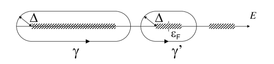
Figure 2: The two contours, $\gamma$ and $\gamma^{\prime}$, surround the states below $\epsilon_{F}^{0}$ and the states split from the Fermi level, respectively, such that the distance from any point on the contours to ${\cal I}$ is equal to some $\Delta>0$.

The last thing we need to prove is that, for $\lambda$ small enough,

$$\|\textsf{T}_{\epsilon}[n]-n_{0}\|_{L^{1}}\leq\epsilon,$$ (28)

for any $n$ in $S^{N,\epsilon}_{sym}$ and $\epsilon$ satisfying Eq. (27). Let us consider

$$\hat{Z}[n]=\int_{\gamma}(z-H_{n})^{-1}\frac{dz}{2\pi i}+P_{\Gamma_{0}}\int_{\gamma^{\prime}}(z-H_{n})^{-1}\frac{dz}{2\pi i},$$ (29)

defined on the entire $S^{N}$. Based on the previous results, we observe that $P_{n}^{<}=\hat{Z}[n]$ for $n\in S^{N,\epsilon}_{sym}$, with $\epsilon$ satisfying Eq. (27). Also, notice that $n_{0}(x)=\hat{Z}[\bar{n}](x,x)$. Moreover, if $\|\ \|_{1}$ denotes the trace norm,

$$\|\hat{Z}[n]-\hat{Z}[n^{\prime}]\|_{1}\leq\frac{\lambda\alpha\chi k_{a}}{(1-\lambda\gamma_{a})^{2}}\|n-n^{\prime}\|_{L^{1}},$$ (30)

with

$$\alpha=\left(\int_{\gamma}+\int_{\gamma^{\prime}}\right)\left(1+\frac{|z+a|}{\Delta}\right)^{2}\frac{|dz|}{2\pi}.$$ (31)

Indeed, let

$$B\equiv(H_{0}+a)^{-1}(V_{n}-V_{n^{\prime}})(H_{0}+a)^{-1},$$ (32)

and $g_{a,z}(t)\equiv(t+a)/(z-t)$. After simple manipulations,

$$\hat{Z}[n]-\hat{Z}[n^{\prime}]=\lambda\left(\int_{\gamma}\frac{dz}{2\pi i}+P_{\Gamma_{0}}\int_{\gamma^{\prime}}\frac{dz}{2\pi i}\right)g_{a,z}(H_{n})\times$$

$$(1+\lambda(H_{0}+a)^{-1}V_{n})^{-1}B(1+\lambda V_{n^{\prime}}(H_{0}+a)^{-1})^{-1}g_{a,z}(H_{n^{\prime}})$$ (33)

and notice that

$$\|g_{a,z}(H_{n})\|\leq 1+\frac{|z+a|}{\Delta},$$ (34)

for all $n\in S^{N}$ and $z\in\gamma$ or $\gamma^{\prime}$. We can conclude at this step that

$$\|\hat{Z}[n]-\hat{Z}[n^{\prime}]\|_{1}\leq\frac{\lambda\alpha}{(1-\lambda\gamma_{a})^{2}}\|B\|_{1}.$$ (35)

If we use the polar decomposition $\Delta V=S|\Delta V|$ of $\Delta V\equiv V_{n}-V_{n^{\prime}}$, and define $A\equiv|\Delta V|^{1/2}(H_{0}+a)^{-1}$, then from Eq. (32)

$$\|B\|_{1}=\|A^{\ast}SA\|_{1}\leq\|A^{*}\|_{HS}\|SA\|_{HS}\leq\|A\|_{HS}^{2},$$ (36)

and

$$\|A\|_{HS}^{2}=\int|\Delta V(x)|(H_{0}+a)^{-2}(x,x)dx\leq k_{a}\chi\|n-n^{\prime}\|_{L^{1}}.$$ (37)

With Eq. (30) proven, we can easily end the proof of i). Indeed, for all $n\in S^{N,\epsilon}_{sym}$,

$$\|\textsf{T}_{\epsilon}[n]-n_{0}\|_{L^{1}}=\|\hat{Z}[n](x,x)-\hat{Z}[\bar{n}](x,x)\|_{L^{1}}$$

$$\leq\|\hat{Z}[n]-\hat{Z}[\bar{n}]\|_{1}\leq\frac{\lambda\alpha\chi k_{a}}{(1-\lambda\gamma_{a})^{2}}\|n-\bar{n}\|_{L^{1}}$$ (38)

and

$$\|n-\bar{n}\|\leq\|n-n_{0}\|+\|n_{0}-\bar{n}\|\leq\epsilon+2N_{0}.$$ (39)

Thus, Eq. (28) is true if

$$\frac{\lambda\alpha\chi k_{a}(2N_{0}+\epsilon)}{(1-\lambda\gamma_{a})^{2}}\leq\epsilon$$ (40)

and we remark that Eqs. (27) and (40) can be simultaneously satisfied if $\lambda$ is small enough.

ii) Observe that if we take $\lambda$ small so as to satisfy Eq. (40), then

$$\frac{\lambda\alpha\chi k_{a}}{(1-\lambda\gamma_{a})^{2}}<1.$$ (41)

Then $\textsf{T}_{\epsilon}$ is a contraction, since $P_{n}^{<}$ and $\hat{Z}[n]$ coincide on $S^{N,\epsilon}_{sym}$ and

$$\|\textsf{T}_{\epsilon}[n]-\textsf{T}_{\epsilon}[n^{\prime}]\|_{L^{1}}\leq\|P_{n}^{<}-P_{n^{\prime}}^{<}\|_{1}$$

$$=\|\hat{Z}[n]-\hat{Z}[n^{\prime}]\|_{1}<\|n-n^{\prime}\|_{L^{1}}.$$ (42)

Since $\textsf{T}_{\epsilon}$ is a contraction on a closed set, it must have one and only one fixed point.

iii) It follows immediately if we express $P_{n}^{<}$ in terms of the eigenvectors and notice that, at a fixed point, $n(x)=P_{n}^{<}(x,x)$:

$$H_{n}\phi_{i}=\epsilon_{i}\phi_{i},\ \ n(x)=\sum\limits_{\epsilon_{i}<\epsilon_{F}^{0}}|\phi_{i}(x)|^{2}.$$ (43)

Together with $\int n(x)dx=N$, the above equations are exactly the KS equations at zero temperature.

3 Examples

We consider first one of the simplest examples possible: $2N$ particles on a circle of length $a$. The Kohn-Sham Hamiltonian is $H_{n}=-\partial_{x}^{2}+V_{n}$, where $x$ is the coordinate along the circle. The ground state of $H_{0}\equiv-\partial_{x}^{2}$ is non-degenerate, while all the excited states are doubly degenerate. Thus, if we populate the states of $H_{0}$ with $2N$ particles, we end up with one particle occupying a double degenerate energy level, containing the states $a^{-1/2}e^{ik_{F}x}$ and $a^{-1/2}e^{-ik_{F}x}$ ($\epsilon_{F}^{0}=k_{F}^{2}$).

We now go over the constructions considered in the previous section. The continuous group $G_{c}$ are the rotations of the circle and the subgroup $G$ can be taken as the identity plus the reflection $r:\ x\rightarrow-x$. There are two, one dimensional irreducible representations of $G$, $\chi_{\pm}(r)t=\pm t$. The projectors $P_{\Gamma}$ ($\Gamma\rightarrow\pm$) are simply given by

$$(P_{\pm}f)(x)=\frac{1}{\sqrt{2}}[f(x)\pm f(-x)].$$ (44)

They decompose ${\cal H}_{F}$ in the invariant, 1 dimensional spaces

$$P_{+}{\cal H}_{F}=\{\sqrt{\frac{2}{a}}\cos k_{F}x\},\ \ P_{-}{\cal H}_{F}=\{\sqrt{\frac{2}{a}}\sin k_{F}x\},$$ (45)

each of them providing an irreducible representation for $G$. Either one of the ($\pm$) representations can chooses as $\Gamma_{0}$ in A6. We choose the (+) representation, in which case, $n_{0}(x)=\bar{n}+a^{-1}\cos(2k_{F}x)$ and condition A7 reads

$$\int V_{n_{0}}(x)\cos(2k_{F}x)dx<0.$$ (46)

In LDA, if we approximate $v_{xc}(n_{0})\simeq v_{xc}(\bar{n})+v_{xc}^{\prime}(\bar{n})(n_{0}-\bar{n})$, Eq. (46) reduces to

$$\hat{v}(2k_{F})+v_{xc}^{\prime}(\bar{n})<0,$$ (47)

where $\hat{v}$ is the Fourier transform of the two-body interaction. For QA, Eq. (46) simply means $\hat{K}(2k_{F})<0$. We will be led to the same conditions on the effective potential if we choose $\Gamma_{0}$ to be the anti-symmetric (-) representation.

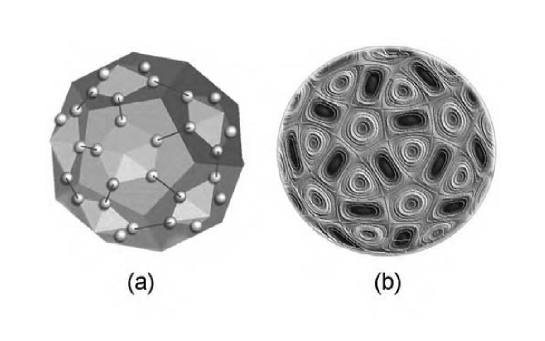
Figure 3: a) The molecular structure of the C₆₀ molecule. The small spheres represent the carbon atoms. The double bonds are indicated by segments joining two atoms. b) A contour plot of the density $n_{0}(x)$ defined in the text. The dark/lighter regions corresponds to high/low densities.

Similar examples can be given for toruses in higher dimensions. We, however, consider the case of fermions on the 2D sphere and show that we can obtain the molecular structure of the C₆₀ molecule. In the C₆₀ molecule, the carbon atoms sit at the points of intersection between an icosahedron and dodecahedron as shown in Fig. 3a. There are single and double bonds between the carbon atoms. Since the double bond is much stronger than the single bond, we consider C=C as being the building blocks of the C₆₀ molecule. In total, there are 30 double bonds and some of them are shown in Fig. 3a. We consider then 30 point particles (of course, we tried 60 particles with no success) on a sphere of radius $R$, described by the Kohn-Sham Hamiltonian $H_{n}=-R^{-2}\vec{L}^{2}+V_{n}$, where $H_{0}=-R^{-2}\vec{L}^{2}$ is the kinetic energy of a particle on the sphere. The energy levels of $H_{0}$ are simply $R^{-2}l(l+1)$, $l=0,\ 1,\ldots$, and if we populate them in order, we end up with 5 particles on the $l=5$ level. The continuous group is $O(3)$ and we can take the proper icosahedral group as the finite subgroup $G$. Indeed, under its action, the Fermi level decomposes as

$${\cal H}_{F}=H_{u}\oplus T_{1u}\oplus T_{2u},$$ (48)

i.e. in a 5 dimensional space plus two 3 dimensional spaces (of different symmetries). Thus, the proper icosahedral group satisfies A5-A6 with $\Gamma_{0}=H_{u}$. Then, if the effective potential satisfies A7 (which we expect to happen for certain radiuses $R$), the Kohn-Sham equations for the 30 particles on the sphere have a stable solution $n(x)=n_{0}(x)+o(\lambda)$, where $n_{0}(x)$ is obtained by populating all $l<5$ levels plus the 5 states with $l=5$ and $H_{u}$ symmetry. This density is shown in Fig. 3b and the resemblance with the C₆₀ molecule is evident.

We end this section with a discussion of the numerical results of Ref. [4] on 2D electrons and a completely deformable jellium, whose electrostatic potential cancels exactly the electrons’ Hartree potential. This system is described by the Kohn-Sham Hamiltonian:

$$H_{n}=-\Delta+\bar{v}_{xc}(n),$$ (49)

where $\bar{v}_{xc}(n)$ is an effective 2D exchange-correlation potential (treated in the local density approximation). From the beginning, we should mention that this system does not fall in our category. We discussed here systems that are confined in finite volumes and the small coupling constant regime. In Eq. (49), the electrons are free to move in the entire 2 dimensional space. The only confining potential is their own exchange-correlation potential. Since this potential needs to bind these electrons, we cannot talk about the small coupling limit. However, we will show that our analysis still applies. We mention that a group analysis of the symmetry breaking in small parabolic quantum dots was already carried in Ref. [8].

The self-consistent numerical solutions of Eq. (49) showed the following: there is a first class of stable crystals, which have pure shapes, like triangles, squares and circles, and there is a second class with apparently no regularity in the shape. We discuss the crystals with pure shape, where the symmetry group is easy to recognize, and the case when the electrons are paired and the spin degree of freedom is not important. Clearly, for the triangle-shaped crystals, the symmetry has been broken to $G=C_{3}v$, the group that sends an equilateral triangle into itself. For the square ones, $G=D_{4v}$, the group that sends a square into itself. In Ref. [4], it was found numerically that crystals with 8 and 10 particles prefer the square geometry. Let us show how one can predict this. We first guess a good density $n^{(0)}$, which is a uniform density inside a square. $n^{(0)}$ will create a constant, (strongly) negative potential inside the square and the electrons will behave, more or less, like they are confined within hard walls. The eigenstates for this system are $\psi_{nm}(x,y)=\frac{2}{A}\sin(n\pi x/L)\sin(m\pi y/L)$ ($L$ the size of the square and $A=L^{2}$). The lowest energy state is $\psi_{11}$. The first excited state is double-degenerate and corresponds to $\psi_{12}$ and $\psi_{21}$: $D_{4v}$ acts irreducibly on this space. The third excited state is non-degenerate and correspond to $\psi_{22}$. The fourth excited state is again double degenerate and corresponds to $\psi_{13}$ and $\psi_{31}$: under the representations of $D_{4v}$, this level decomposes into 2 invariant, 1 dimensional spaces (symmetric and anti-symmetric combinations of $\psi_{13}$ and $\psi_{31}$). Thus, with 8 particles, we can populate the first 3 levels and have the closed shell condition. Thus, the self-consistency can be achieved without further reduction of the symmetry. If we write $H_{0}=-\Delta+\bar{v}_{xc}(n^{(0)})$, we reduced the Kohn-Sham Hamiltonian to $H_{n}=H_{0}+V_{n}$, where $H_{0}$ describes, more or less, free electrons confined in the square and $V_{n}=\bar{v}_{xc}(n)-\bar{v}_{xc}(n^{(0)})$ can be considered small. The density $n_{0}$ of our theorem is given by populating the first 3 energy levels of $H_{0}$ and proving the existence of a self-consistent solution near $n_{0}$ may be accomplished now with the methods developed in this paper. The self-consistent field will split the fourth energy level, so we can accommodate another pair of electrons without breaking the symmetry, i.e. the crystal with 10 electrons should also have square symmetry. Examining either Fig. 2 or the inset of Fig. 3 (where one can see the splitting of the second energy level) in Ref. [4], it follows that, in reality, there is a slight deviation from the $D_{4v}$ symmetry.

4 Discussion

We can summarize our procedure as follows (hopefully this can be seen in the above examples): in the first part, one looks for $n_{0}$, which must be a good approximation of the self-consistent density. The main goal is to fulfill the closed shell condition and group theoretical methods can be used to accomplish that. After $n_{0}$ is found, one can construct the map T in a neighborhood of $n_{0}$. In the second part, one investigates if T is indeed a contraction near $n_{0}$. For small $\lambda$, the conditions in which this is true are already given here. How large this $\lambda$ can be depends on $V_{n}$ and its derivative near $n_{0}$.

One important remark is that some of these non-uniform solutions can be found only if we start the iteration close enough to them. The reason is that the basin of attraction of the map T may be small (notice that the usual iterative process of solving KS equations consists exactly in constructing the sequence $n_{0}$, $\textsf{T}[n_{0}]$, $\ldots$, $\textsf{T}^{m}[n_{0}]$, etc.). For this reason, there may be additional isomers to the ones found in Ref. [4].

As opposed to the Jahn-Teller effect [9] or Pierls instability [10], which involves discrete symmetries and the electronic degeneracies are lifted by a displacement of the atoms, the symmetry breaking discussed here involves a continuous group and is due solely to the electron-electron interaction, which lifts the electronic degeneracies without any change in the external potential. The Jahn-Teller and Pierls instabilities may be triggered (but not necessarily) by the instability we discussed here.

Our analysis does not rule out the existence of more than one self-consistent solution of the KS equations. The lowest energy configuration is, of course, associated with the ground state, and the higher energy configurations should be associated with excited states. In Ref. [7], the authors find that indeed, since the energy functional $E_{v}[n]$ is not convex, $E_{v}[n]$ may have additional extrema, which are excited-state densities.

Degeneracy and symmetry breaking in DFT are well studied concepts in Density Functional Theory [11, 12], and there are many numerical studies on the subject. In fact, the modern theory of freezing [13], which can be traced back to the pioneering work of Ramakrishnan and Yussouff [14], is based on the assumption that the liquid-solid transitions occurs because of a bifurcation of the same type as we discussed here. More exactly, the density of the solid $n_{s}$ is computed self-consistently as the linear response of the uniform liquid density $n_{l}$ to the introduction of a density change $\Delta n=n_{s}-n_{l}$. In the current state, the procedure cannot predict the lattice symmetry, but rather assumes that the linear response equation has a non-uniform solution, with a prescribed crystalline symmetry (usually known from experiment). Applied to quantum liquids, this procedure is equivalent to solving the Kohn-Sham equations in the quadratic approximation. One can find in Ref. [15] an impressive numerical demonstration of the Wigner crystallization of the electron liquid. For finite systems, we already mentioned Refs. [4] and [8]. We add Refs. [16] and [17].

We also want to mention that Bach et al [18] have shown that, for any repulsive interaction, the energy levels are always fully occupied in the unrestricted Hartree-Fock approximation. This result automatically implies that there must be a symmetry breaking whenever the last occupied level of $H_{0}$ is only partially populated. In contradistinction, Ref. [19] showed that, within the Hartree approximation (1D), there is always a symmetry breaking for short, attractive interactions. This definitely shows that we have to go beyond the two approximations.

At the end, we want to mention that we have partial but interesting results in the thermodynamic limit and we are currently considering the finite temperature regime. We are also looking into the spin case, when the Kohn-Sham equations become self-consistent equations for the density $n(x)$ and magnetization vector $\vec{m}(x)$.

References

- [1] Kohn, W. and Sham, L.J., Phys. Rev. 140, (1965) A1133.
- [2] Mermin, N.D., Phys. Rev 137, (1965) A1441.
- [3] Kohn, W., Rev. Mod. Phys. 71, (1999) 1253.
- [4] S.M. Reiman et al, Phys. Rev. B 58, (1998) 8111.
- [5] Prodan, E. and Nordlander P., J. of Stat. Phys. 111, (2003) 967.
- [6] Prodan, E. and Nordlander P., J. of Math. Phys. 42, (2001) 3390.
- [7] Perdew, J.P and Levy, M., Phys. Rev. B 31, (1995) 6264.
- [8] Yannouleas, C. and Landman, U., Phys. Rev. B 68, (2003) 035325.
- [9] Jahn, H.A. and Teller, E., Proc. Roy. Soc. A161, (1937) 220.
- [10] Peierls, R.E.: it Quantum theory of solids, (Clarendon, Oxford 1955).
- [11] Savin, A., Recent development and applications of Density Functional Theory, (Elsevier, Amsterdam, 1996, p. 327).
- [12] Perdew, J.P., Savin, A. and Burke, K., Phys. Rev. A 51, (1995) 4531.
- [13] Baus, M., J. Phys.: Condens. Matter 2, (1990) 2111.
- [14] Ramakrishnan, T.V. and Yussouff, M., Phys. Rev. B 19, (1979) 2775.
- [15] Likos, C. N., Moroni, S. and Senatore, G., Phys. Rev. B 55, (1997) 8867.
- [16] Filinov, A.V., Bonitz, M. and Lozovik, Y.E., Phys. Rev. Lett. 86, (2001) 3851.
- [17] Yannouleas, C. and Landman, U., Phys. Rev. Lett. 82, (1999) 5325.
- [18] Bach, V., Lieb, E.H., Loss, M. and Solovej, J.P., Phys. Rev. Lett. 72, (1994) 2981.
- [19] Prodan, E. and Nordlander, P., J. Math. Phys. 42, (2001) 3424.