Nonsingular stress and strain fields of dislocations and disclinations in first strain gradient elasticity

Abstract

The aim of this paper is to study the elastic stress and strain fields of dislocations and disclinations in the framework of Mindlin’s gradient elasticity. We consider simple but rigorous versions of Mindlin’s first gradient elasticity with one material length (gradient coefficient). Using the stress function method, we find modified stress functions for all six types of Volterra defects (dislocations and disclinations) situated in an isotropic and infinitely extended medium. By means of these stress functions, we obtain exact analytical solutions for the stress and strain fields of dislocations and disclinations. An advantage of these solutions for the elastic strain and stress is that they have no singularities at the defect line. They are finite and have maxima or minima in the defect core region. The stresses and strains are either zero or have a finite maximum value at the defect line. The maximum value of stresses may serve as a measure of the critical stress level when fracture and failure may occur. Thus, both the stress and elastic strain singularities are removed in such a simple gradient theory. In addition, we give the relation to the nonlocal stresses in Eringen’s nonlocal elasticity for the nonsingular stresses.

Keywords: gradient theory, dislocations, disclinations, nonlocal elasticity, hyperstress

1 Introduction

The traditional methods of classical elasticity break down at small distances from crystal defects and lead to singularities. This is unfortunate since the defect core is an important region in the theory of defects. Moreover, such singularities are unphysical and an improved model of defects should eliminate them. In addition, classical elasticity is a scale-free continuum theory in which no characteristic length appears. Therefore, the classical elasticity cannot explain the phenomena near defects and at atomic scale.

An extension of the classical elasticity is the so-called strain gradient elasticity. The physical motivation to introduce gradient theories was originally given by Kröner [1, 2] in the early sixties. The strain gradient theories extend the classical elasticity with additional strain gradient terms. Due to the gradients, they must contain additional material constants with the dimension of a length, and hyperstresses appear. The hyperstress tensor is a higher order stress tensor given in terms of strain gradients. In particular, the isotropic, higher-order gradient, linear elasticity was developed essentially by Mindlin [3, 4, 5], Green and Rivlin [6, 7] and Toupin [8] (see also [9, 10, 11]). Strain gradient theories contain strain gradient terms and no rotation vector and no proper couple-stresses appear. In this way, they are different from theories with couple-stresses and Cosserat theory (micropolar elasticity). Only hyperstresses such as double or triple stresses appear in strain gradient theories. Double stresses correspond to a force dipole and triple stresses belong to a force quadrupole. The next order would corresponds to a force octupole.

Stress and Hyperstress are physical quantities in a 3-dimensional continuum mechanics. Within a framework of the 4-dimensional spacetime continuum, stress and hyperstress translate into momentum and hypermomentum [12, 13].

In the present work, we consider two simple but straightforward versions of a first strain gradient theory. We investigate screw and edge dislocations and wedge and twist disclinations in the framework of incompatible strain gradient elasticity. We apply the “modified” stress function method to these types of straight dislocations and disclinations. Using this method, we derive exact analytical solutions for the stress and strain fields demonstrating the elimination of “classical” singularities from the elastic field at the dislocation and disclination line. Therefore, stresses and strains are finite within this gradient theory. We obtain “modified” stress functions for all types of straight dislocations and disclinations. In addition, we justify that these solutions are solutions in this special version of Mindlin’s first gradient elasticity. We also give the relation of nonsingular stresses of dislocations and disclinations to Eringen’s nonlocal elasticity theory. We show that these stresses correspond to the “nonlocal” stresses.

2 Governing equations

Following Mindlin [3, 4, 5] (see also [10]), we start with the strain energy in gradient elasticity of an isotropic material. We only consider first gradients of the elastic strain in this paper. In the small strain gradient theory the strain energy, $W$, is assumed to be a function

$$W=W(E_{ij},\partial_{k}E_{ij})$$ (1)

of the elastic strain, $E_{ij}$, and the gradient of the elastic strain, $\partial_{k}E_{ij}$, which is sometimes called hyperstrain. The $E_{ij}$ is dimensionless and the $\partial_{k}E_{ij}$ has the dimension of the reciprocal of length. Obviously, no elastic rotation and gradients of it appear in (1). The elastic strain can be a gradient of the displacement $u_{i}$

$$E_{ij}=\partial_{(i}u_{j)}=\frac{1}{2}\big{(}\partial_{i}u_{j}+\partial_{j}u_{i}\big{)}$$ (2)

or can have the following form [14, 15, 16, 17, 18, 19]

$$E_{ij}=\partial_{(i}u_{j)}+\tilde{\beta}_{(ij)},\qquad E_{ij}=E_{ji}$$ (3)

where $\tilde{\beta}_{(ij)}$ denotes the incompatible part of the elastic strain. In addition, the negative incompatible strain may be identified as the plastic strain ($\beta^{P}_{(ij)}\equiv-\tilde{\beta}_{(ij)}$). The strain (2) is the elastic strain in a compatible situation. On the other hand, (3) corresponds to the elastic strain for the incompatible case (e.g. dislocations and disclinations). In the incompatible situation the $u_{i}$ and $\tilde{\beta}_{ij}$ are not “good” physical quantities because they are discontinuous functions. Thus, they cannot be physical state quantities. Because the elastic strain is a physical state quantity, it must be a continuous function. It is worth to note that the incompatible strain (3) is similar in form to Mindlin’s so-called relative strain which contains a micro-strain term. But in our case this part is identified as the incompatible elastic strain. Thus, we deal with a theory of incompatible strain gradient elasticity.

The most general form of the strain energy for a linear, isotropic, gradient-dependent elastic material is given by [3, 4]

$$W =\frac{1}{2}\lambda E_{ii}E_{jj}+\mu E_{ij}E_{ij}+c_{1}\big{(}\partial_{j}E_{ij}\big{)}\big{(}\partial_{k}E_{ik}\big{)}+c_{2}\big{(}\partial_{k}E_{ii}\big{)}\big{(}\partial_{j}E_{jk}\big{)}$$

$$\quad+c_{3}\big{(}\partial_{k}E_{ii}\big{)}\big{(}\partial_{k}E_{jj}\big{)}+c_{4}\big{(}\partial_{k}E_{ij}\big{)}\big{(}\partial_{k}E_{ij}\big{)}+c_{5}\big{(}\partial_{k}E_{ij}\big{)}\big{(}\partial_{i}E_{jk}\big{)}.$$ (4)

The constants $\lambda$ and $\mu$ are the Lamé constants and the five $c_{n}$ are the additional constants (gradient coefficients) which appear in Mindlin’s strain gradient theory [3, 4]. Thus, five strain gradient terms  appear in the isotropic case.

On the one hand, the Cauchy stress tensor is defined as (Hooke’s law)

$$\sigma_{ij}:=\frac{\partial W}{\partial E_{ij}}=\lambda\delta_{ij}E_{kk}+2\mu E_{ij}$$ (5)

and has the symmetry $\sigma_{ij}=\sigma_{ji}$. The elastic stress has the dimension of force, $F_{i}$, per unit area ${\mathrm{d}}A_{j}$. In addition, the elastic energy is completely symmetric in the strain and stress tensor so that the condition for the strain follows

$$E_{ij}=\frac{\partial W}{\partial\sigma_{ij}}=\frac{1}{2\mu}\,\Big{(}\sigma_{ij}-\frac{\nu}{1+\nu}\delta_{ij}\sigma_{kk}\Big{)},$$ (6)

with $\lambda=2\mu\nu/(1-2\nu)$.

On the other hand, the hyperstress tensor is defined as follows (see also [3, 4])

$$\tau_{ijk}:=\frac{\partial W}{\partial\big{(}\partial_{k}E_{ij}\big{)}} =c_{1}\big{(}\delta_{ki}\partial_{l}E_{lj}+\delta_{kj}\partial_{l}E_{li}\big{)}+\frac{1}{2}\,c_{2}\big{(}\delta_{ki}\partial_{j}E_{ll}+\delta_{kj}\partial_{i}E_{ll}+2\delta_{ij}\partial_{l}E_{lk}\big{)}$$

$$\quad+2c_{3}\delta_{ij}\partial_{k}E_{ll}+2c_{4}\partial_{k}E_{ij}+c_{5}\big{(}\partial_{i}E_{jk}+\partial_{j}E_{ik}\big{)}.$$ (7)

It has the character of double forces per unit area. The dipolar or double force acts through that area. In this case $\tau_{ijk}$ is a dipolar or double stress tensor. The first index of $\tau_{ijk}$ describes the orientation of the pair of forces $F_{i}$, the second index gives the orientation of the lever arm $\Delta x_{j}$ between the forces and the third index denotes the orientation of the normal $n_{k}$ of the plane on which the stress acts (see Fig. 1).

Figure 1: Double force stress $\tau_{ijk}$ acting on a plane with normal $n_{k}$.

The double stress gives a contribution in the compatible as well as the incompatible case. In strain gradient theory it has the symmetry

$$\tau_{ijk}\equiv\tau_{(ij)k}=\frac{1}{2}\big{(}\tau_{ijk}+\tau_{jik}\big{)},$$ (8)

and possesses 18 components. Thus, the symmetric part $\tau_{(ij)k}$ arises from double forces without moment (see Fig. 2a). It can be resolved into the dilatational double stress $\tau_{llk}$ and the traceless symmetric double stress $\tau_{(ij)k}-\frac{1}{3}\delta_{ij}\tau_{llk}$. No antisymmetric double stresses $\tau_{[ij]k}$, which arise from double forces with moment (couple stresses), appear

$$\tau_{[ij]k}=\frac{1}{2}\big{(}\tau_{ijk}-\tau_{jik}\big{)}=0,$$ (9)

which would correspond to rotation-gradients (see Fig. 2b). In general, a couple stress tensor has 9 components.

(a)

(b)

Figure 2: Double force stresses (a) $\tau_{(yx)k}$ and (b) $\tau_{[yx]k}$ acting on a plane with normal $n_{k}$.

For vanishing external body forces, the force equilibrium equation can be derived from the principle of virtual work as (variation with respect to the displacement) [3]

$$\partial_{j}\big{(}\sigma_{ij}-\partial_{k}\tau_{ijk}\big{)}=0.$$ (10)

Since we consider an infinitely extended medium, we may neglect additional boundary conditions. With Eqs. (5) and (2), the force equilibrium (10) reads

$$\partial_{j}\Big{(}\lambda\delta_{ij}E_{kk}+2\mu E_{ij}-(c_{1}+c_{5})\big{(}\partial_{i}\partial_{l}E_{lj}+\partial_{j}\partial_{l}E_{li}\big{)}-c_{2}\big{(}\partial_{i}\partial_{j}E_{ll}+\delta_{ij}\partial_{k}\partial_{l}E_{lk}\big{)}$$

$$-2\big{(}c_{3}\delta_{ij}\Delta E_{kk}+c_{4}\Delta E_{ij}\big{)}\Big{)}=0,$$ (11)

where $\Delta$ denotes the Laplacian. Such an expression (2) is quite formidable and hard to solve. Thus, a physical simplification could be useful.

First possibility of simplification: Let us follow a way in gradient elasticity similar to the way which Feynman [20] went in linear gravity. He pointed out that not all five gradient terms are necessary. Because the gradient term to $c_{5}$ can be converted to the $c_{1}$ gradient term by integration by parts. Therefore, the $c_{5}$ term may be omitted. We set $c_{5}=0$. In addition, the Cauchy stress tensor should fulfill an equilibrium condition of the kind as in elasticity

$$\partial_{j}\sigma_{ij}=0.$$ (12)

Consequently, in (10) it must yield

$$\partial_{k}\partial_{j}\tau_{ijk}=0,$$ (13)

and $\tau_{ijk}$ is self equilibrating. Using (2) and $c_{5}=0$, Eq. (13) reads

$$c_{1}\big{(}\partial_{i}\partial_{j}\partial_{l}E_{lj}+\Delta\partial_{l}E_{li}\big{)}+c_{2}\big{(}\partial_{i}\Delta E_{ll}+\partial_{i}\partial_{k}\partial_{l}E_{lk}\big{)}+2\big{(}c_{3}\partial_{i}\Delta E_{kk}+c_{4}\partial_{j}\Delta E_{ij}\big{)}=0.$$ (14)

It may be solved by

$$\partial_{i}\partial_{j}\partial_{l}E_{jl}\big{(}c_{1}+c_{2}\big{)} =0,$$

$$\Delta\partial_{l}E_{il}\big{(}c_{1}+2c_{4}\big{)} =0,$$

$$\Delta\partial_{i}E_{ll}\big{(}c_{2}+2c_{3}\big{)} =0.$$ (15)

If we choose a scale such that $c_{4}=\ell/2$, then the solution of (2) is given by

$$c_{1}=-\ell,\qquad c_{2}=\ell,\qquad c_{3}=-\frac{\ell}{2},\qquad c_{4}=\frac{\ell}{2}.$$ (16)

The coefficient $\ell$ has the dimension of a force. Thus, the coefficient $\ell$ may be chosen

$$\ell=\frac{2\mu}{\kappa^{2}}$$ (17)

with only one “gradient-coefficient” or “parameter of nonlocality”

$$\kappa^{-2}>0.$$ (18)

$\kappa^{2}$ has the dimension of $1/[{\text{length}}^{2}]$. It is a positive material constant. What we have recovered is nothing but the so-called Einstein choice in three dimensions scaled by a factor $\ell$ (see, e.g., [21, 17]). So, we can write down the expression

$$\frac{1}{\ell}\,\partial_{k}\tau_{ijk} =\left(\text{inc}\,\boldsymbol{E}\right)_{ij}\equiv-\epsilon_{ikl}\epsilon_{jmn}\partial_{k}\partial_{m}E_{ln}$$

$$=\Delta E_{ij}-(\partial_{j}\partial_{k}E_{ik}+\partial_{i}\partial_{k}E_{kj})+\delta_{ij}\partial_{k}\partial_{l}E_{kl}+\partial_{i}\partial_{j}E_{kk}-\delta_{ij}\Delta E_{kk}$$ (19)

which is equivalent to the three dimensional linear Einstein tensor. The linear Einstein tensor is the incompatibility of the strain (see [22, 23]). Thus, the three dimensional Einstein tensor is proportional to the divergence of the double force stress tensor. The Einstein choice has been used in the gauge theory of dislocations by Lazar [24, 17, 18] and by Malyshev [25]. Eq. (2) leads to physical solutions for the screw dislocation [17, 18, 25]. The solution of an edge dislocation [25] has a modified far field of the stress. In fact, it does not coincide with the far field of the classical solution. One way out is to modify the strain energy with additional bend-twist terms [19]. But then we are leaving the framework of strain gradient elasticity which is not our aim. Anyway, it is interesting to note that the three dimensional Einstein choice which is used in the gauge theory of dislocations is contained in the strain energy expression (2) given by Mindlin.

Second possibility of simplification: If we require that the stress-strain symmetry of the elastic energy should also be valid for the gradient terms, and we think this is quite natural, we have to use the following choice of the five gradient coefficients

$$c_{1}=0,\quad c_{2}=0,\quad c_{3}=\frac{\lambda}{2\kappa^{2}},\quad c_{4}=\frac{\mu}{\kappa^{2}},\quad c_{5}=0.$$ (20)

Then the strain energy can be rewritten in the following simple form

$$W=\frac{1}{2}\,\sigma_{ij}E_{ij}+\frac{1}{2\kappa^{2}}\,\big{(}\partial_{k}\sigma_{ij}\big{)}\big{(}\partial_{k}E_{ij}\big{)}.$$ (21)

One can see that $\kappa$ has the dimension of an inverse length. Thus, by using the special choice (20), we have obtained a simple but still rigorous version of Mindlin’s gradient theory which is a simple strain gradient as well as stress gradient theory. In particular, the elastic energy (21) is symmetric with respect to the strain and the stress and also with respect to the strain gradient and the stress gradient

$$\frac{\partial W}{\partial(\partial_{k}E_{ij})}=\frac{1}{\kappa^{2}}\,\partial_{k}\sigma_{ij},\qquad\frac{\partial W}{\partial(\partial_{k}\sigma_{ij})}=\frac{1}{\kappa^{2}}\,\partial_{k}E_{ij}.$$ (22)

Then the double stress tensor has the following form

$$\tau_{ijk}=\frac{1}{\kappa^{2}}\,\partial_{k}\sigma_{ij}=\frac{1}{\kappa^{2}}\,\big{(}2\mu\partial_{k}E_{ij}+\lambda\delta_{ij}\partial_{k}E_{ll}\big{)}.$$ (23)

Consequently, the double stress (23) is a simple gradient of the Cauchy stress. Thus, it is a higher-order stress tensor. Only $\kappa^{-2}$ is a non-standard coefficient of the theory. Recently, double stresses similar in their form to (23) have also been used in the mode-I crack problem [26] and the mode-III crack problem [27, 28].

Let us mention that a higher order gradient elastic energy with the required symmetry would have the following form

$$W =\frac{1}{2}\,\sigma_{ij}E_{ij}+\frac{1}{2\kappa^{2}}\,\big{(}\partial_{k}\sigma_{ij}\big{)}\big{(}\partial_{k}E_{ij}\big{)}+\frac{1}{2\hat{\kappa}^{4}}\,\big{(}\partial_{l}\partial_{k}\sigma_{ij}\big{)}\big{(}\partial_{l}\partial_{k}E_{ij}\big{)}$$

$$\quad+\frac{1}{2\tilde{\kappa}^{6}}\,\big{(}\partial_{m}\partial_{l}\partial_{k}\sigma_{ij}\big{)}\big{(}\partial_{m}\partial_{l}\partial_{k}E_{ij}\big{)}+\cdots,$$ (24)

where $\hat{\kappa}$ and $\tilde{\kappa}$ are higher order gradient coefficients. It is interesting to note that the last term in Eq. (2) with the third strain gradient corresponds to a force octupole. But in the following we only consider the first gradient theory given by (21).

In addition, we note that Altan and Aifantis [29] have used a similar choice like (20) for the study of cracks within their version of strain gradient elasticity. Anyway, they did not use the notion of double stress. For that reason, they identified the Cauchy stress with the total stress tensor. The price they had to pay was that the singularities are still present in the stresses. In order to regularize both the elastic strain and the stress singularities Ru and Aifantis [41] (see also [42]) introduced a constitutive relation with gradients of the elastic strain and the stress multiplied by two different gradient coefficients. In our framework, which we use in this paper, it is not necessary to introduce such a constitutive relation because the Cauchy stress is defined as the derivative of the strain energy with respect to the elastic strain and nothing else. On the other hand, Gutkin and Aifantis [30] used another choice so that no double stresses appear. But, on the other hand, triple stresses which correspond to second gradient strain must appear in their approach and, therefore, in the equilibrium equations. But they neglected the triple stresses which is not straightforward. The strain gradient elasticity which contains two different gradient coefficients proposed by Ru and Aifantis [31] is used by Gutkin and Aifantis [32, 33, 34] for dislocations and disclinations.

By substituting (23) into (10), we obtain

$$\big{(}1-\kappa^{-2}\Delta\big{)}\partial_{j}\sigma_{ij}=0.$$ (25)

If we define

$$\overset{\kern 1.0pt\circ}{\sigma}_{ij}=\sigma_{ij}-\partial_{k}\tau_{ijk}=\lambda\delta_{ij}E_{ll}+2\mu E_{ij}-\kappa^{-2}\big{(}\lambda\delta_{ij}\Delta E_{ll}+2\mu\Delta E_{ij}\big{)},$$ (26)

Eq. (25) takes the form

$$\partial_{j}\overset{\kern 1.0pt\circ}{\sigma}_{ij}=0.$$ (27)

The stress tensor $\overset{\kern 1.0pt\circ}{\sigma}_{ij}$ may be called total stress tensor, which is a kind of “balanced stress”. In the gauge theory of defects it is identified as the background stress tensor. One other difference with Gutkin and Aifantis’ approach [30] is that they consider (26) as a modified constitutive relation while we obtained (26) as field equation instead.

On the other hand, in the incompatible situation we have the additional field $\tilde{\beta}_{ij}$. Which equation corresponds to this field? One should obtain Eq. (26) as a variation of strain energy with respect to $\tilde{\beta}_{ij}$. But so far this does not work. The way out is to add an additional strain energy part to (21),

$$W^{\prime}=-\overset{\kern 1.0pt\circ}{\sigma}_{ij}E_{ij},$$ (28)

which in the compatible situation is a null Lagrangian such that it gives no contribution in the variation with respect to the displacement. The nontrivial traction boundary problems in the variational formulation of field theory can be formulated by means of a null Lagrangian. This procedure is well-known in the gauge theory of dislocations [15, 16, 17, 18, 19, 25]. When the null Lagrangian is added to the elastic Lagrangian (strain energy) it does not change the Euler-Lagrange equation (force equilibrium) because the associated Euler-Lagrange equation, $\partial_{j}\overset{\kern 1.0pt\circ}{\sigma}_{ij}=0$, must be identically satisfied. Then for the incompatible case, Eq. (26) may be considered as the field equation corresponding to $\tilde{\beta}_{ij}$. It is interesting that (26) appears in the compatible as well as the incompatible situation. Only the interpretation of (26) is different.

Now we rewrite Eq. (26) and obtain an inhomogeneous Helmholtz equation for every component of the Cauchy stress

$$\big{(}1-\kappa^{-2}\Delta\big{)}\sigma_{ij}=\overset{\kern 1.0pt\circ}{\sigma}{}_{ij}.$$ (29)

Since the factor $\kappa^{-1}$ has the physical dimension of a length, it defines an internal characteristic length in quite a natural way. It is worth to note that Eq. (29) agrees with the field equation for the nonlocal stress in Eringen’s nonlocal elasticity [35, 36, 37, 38] and for the stress in the gradient elasticity given by Gutkin and Aifantis [32, 33, 34]. If we consider dislocations and disclinations which have an axial symmetry, Eq. (29) may be rewritten as a convolution integral

$$\sigma_{ij}(r)=\int_{V}\alpha(r-r^{\prime})\,\overset{\kern 1.0pt\circ}{\sigma}{}_{ij}(r^{\prime})\,{\mathrm{d}}v(r^{\prime}),$$ (30)

with the corresponding two-dimensional Green’s function

$$\alpha(r-r^{\prime}) =\frac{\kappa^{2}}{2\pi}\,K_{0}\big{(}\kappa\sqrt{(x-x^{\prime})^{2}+(y-y^{\prime})^{2}}\big{)}.$$ (31)

Here $K_{n}$ is the modified Bessel function of the second kind and $n=0,1,\ldots$ denotes the order of this function. In comparison with Eringen’s nonlocal theory of elasticity the Green function (31) may be identified as a nonlocal kernel introduced by Ari and Eringen [39]. Using the inverse of Hooke’s law for the stress $\sigma_{ij}$ and $\overset{\kern 1.0pt\circ}{\sigma}{}_{ij}$, it follows that the elastic strain can be determined from the equation

$$\big{(}1-\kappa^{-2}\Delta\big{)}E_{ij}=\overset{\kern 1.0pt\circ}{E}{}_{ij},$$ (32)

where $\overset{\kern 1.0pt\circ}{E}{}_{ij}$ is the classical strain tensor. Because the strain tensor fulfills an inhomogeneous Helmholtz equation, we may rewrite (32) as a nonlocal relation for the strain

$$E_{ij}(r)=\int_{V}\alpha(r-r^{\prime})\,\overset{\kern 1.0pt\circ}{E}{}_{ij}(r^{\prime})\,{\mathrm{d}}v(r^{\prime}).$$ (33)

Of course, such a relation (33) does not appear in Eringen’s theory [38] of nonlocal elasticity. In his theory, the displacement and the elastic strain are the same as in classical elasticity. Using Hooke’s law, we can combine (29) and (32) to a gradient like relation

$$\big{(}1-\kappa^{-2}\Delta\big{)}\sigma_{ij}=\big{(}1-\kappa^{-2}\Delta\big{)}\big{(}\lambda\delta_{ij}E_{kk}+2\mu E_{ij}\big{)}.$$ (34)

It is interesting to note that Eq. (34) has the same form as the gradient constitutive relation given in [31] if their two different gradient coefficients are the same gradient coefficients. For modified solutions of the stress and elastic strain fields we require that the far field of them should agree with the classical expressions and they should be free from the classical singularities at the defect line. Therefore, we are looking for nonsingular solutions for both the stress and the elastic strain. It depends on the taste of the reader to consider alternatively such constraints as physically motivated boundary conditions.

Using the decomposition (3), we obtain the coupled partial differential equation

$$\big{(}1-\kappa^{-2}\Delta\big{)}\big{[}\partial_{(i}u_{j)}-\beta^{P}_{(ij)}\big{]}=\partial_{(i}\overset{\kern 1.0pt\circ}{u}{}_{j)}-\overset{\kern 1.0pt\circ}{\beta}{}^{P}_{(ij)},$$ (35)

where $\overset{\kern 1.0pt\circ}{u}{}_{i}$ denotes the displacement field and $\overset{\kern 1.0pt\circ}{\beta}{}^{P}_{ij}$ is the plastic distortion in classical defect theory (see, e.g., [14]). Thus, if the following equations are fulfilled

$$\big{(}1-\kappa^{-2}\Delta\big{)}\beta_{ij}=\overset{\kern 1.0pt\circ}{\beta}{}_{ij},$$ (36)

$$\big{(}1-\kappa^{-2}\Delta\big{)}\beta^{P}_{ij}=\overset{\kern 1.0pt\circ}{\beta}{}^{P}_{ij},$$ (37)

the equation for the displacement field ,

$$\big{(}1-\kappa^{-2}\Delta\big{)}u_{i}=\overset{\kern 1.0pt\circ}{u}{}_{i},$$ (38)

is valid for the incompatible case. Thus, for defects (dislocations, disclinations) the inhomogeneous parts of Eqs. (37) and (38) are fields with discontinuities (jumps). We note that Eq. (38) was used by Gutkin and Aifantis [43, 44, 32] in order to calculate the displacement fields for screw and edge dislocations.

In nonlocal elasticity Eringen [35, 36, 37, 38] found the two-dimensional kernel (31) by giving the best match with the Born-Kármán model of the atomic lattice dynamics and the phonon dispersion curves. The length, $\kappa^{-1}$, may be selected to be proportional to the lattice parameter $a$ for a single crystal, i.e.

$$\kappa^{-1}=e_{0}\,a,$$ (39)

where $e_{0}$ is a non-dimensional constant [36]. Obviously, for $e_{0}=0$ we recover classical elasticity. Eringen [35, 36] used the value of $e_{0}=0.39$ in nonlocal elasticity.

We notice that a negative gradient coefficient $\kappa^{-2}<0$ would change the character of the Helmholtz equations (29) and (32) and the corresponding solutions. Let us emphasize that the solutions which we consider in the following sections are valid for a positive gradient coefficient. In addition, non-negative definiteness of the strain energy (21), $W\geq 0$, requires the following conditions for the material constants and the gradient coefficient (see, e.g., [45])

$$3\lambda+2\mu\geq 0,\qquad\mu\geq 0,\qquad\kappa^{-2}\geq 0.$$ (40)

3 Dislocations

In this section we consider straight dislocations whose line coincides with the $z$-axis of a Cartesian coordinate system in an infinitely extended medium.

3.1 Screw dislocation: ${\boldsymbol{b}}=(0,0,b_{z})$

We start with the simplest case, the anti-plane strain which corresponds to a screw dislocation. We make an ansatz for the total stress and for the Cauchy stress which has the form as

$$\overset{\kern 1.0pt\circ}{\sigma}{}_{ij}=\left(\begin{array}[]{ccc}0&0&-\partial_{y}\overset{\kern 1.0pt\circ}{F}\\ 0&0&\partial_{x}\overset{\kern 1.0pt\circ}{F}\\ -\partial_{y}\overset{\kern 1.0pt\circ}{F}&\partial_{x}\overset{\kern 1.0pt\circ}{F}&0\end{array}\right),\quad\sigma_{ij}=\left(\begin{array}[]{ccc}0&0&-\partial_{y}F\\ 0&0&\partial_{x}F\\ -\partial_{y}F&\partial_{x}F&0\end{array}\right).$$ (47)

We choose for $\overset{\kern 1.0pt\circ}{F}$ the well-known stress function of elastic torsion, sometimes called Prandtl’s stress function. It is given by (see, e.g., [23])

$$\overset{\kern 1.0pt\circ}{F}=\frac{\mu b_{z}}{2\pi}\,\ln r,$$ (48)

with $r=\sqrt{x^{2}+y^{2}}$. Substituting (47) and (48) into (29) we obtain for the stress function $F$ the following inhomogeneous Helmholtz equation

$$\Big{(}1-\kappa^{-2}\Delta\Big{)}F=\frac{\mu b_{z}}{2\pi}\,\ln r.$$ (49)

The nonsingular solution of (49) is (see, e.g., [37, 16, 18])

$$F=\frac{\mu b_{z}}{2\pi}\Big{\{}\ln r+K_{0}(\kappa r)\Big{\}},$$ (50)

which represents a stress function for a nonsingular screw dislocation. In the far field, the stress function (50) agrees with Prandtl’s stress function and for small $r$ it cancels the logarithmic singularity. Consequently, the elastic stress is given by

$$\sigma_{zx}=-\frac{\mu b_{z}}{2\pi}\,\frac{y}{r^{2}}\Big{\{}1-\kappa rK_{1}(\kappa r)\Big{\}},\qquad\sigma_{zy}=\frac{\mu b_{z}}{2\pi}\,\frac{x}{r^{2}}\Big{\{}1-\kappa rK_{1}(\kappa r)\Big{\}},$$ (51)

the corresponding field of elastic strains reads

$$E_{zx}=-\frac{b_{z}}{4\pi}\,\frac{y}{r^{2}}\Big{\{}1-\kappa rK_{1}(\kappa r)\Big{\}},\qquad E_{zy}=\frac{b_{z}}{4\pi}\,\frac{x}{r^{2}}\Big{\{}1-\kappa rK_{1}(\kappa r)\Big{\}}.$$ (52)

The appearance of the modified Bessel function in (51) and (52) leads to the elimination of classical singularity $\sim r^{-1}$ at the dislocation line (see Eq. (A.2) in Appendix A). The stress $\sigma_{zy}$ has its extreme value $|\sigma_{zy}(x,0)|\simeq 0.399\kappa\frac{\mu b_{z}}{2\pi}$ at $|x|\simeq 1.114\kappa^{-1}$, whereas the stress $\sigma_{zx}$ has its extreme value $|\sigma_{zx}(0,y)|\simeq 0.399\kappa\frac{\mu b_{z}}{2\pi}$ at $|y|\simeq 1.114\kappa^{-1}$. The strain $E_{zy}$ has its extreme value $|E_{zy}(x,0)|\simeq 0.399\kappa\frac{b_{z}}{4\pi}$ at $|x|\simeq 1.114\kappa^{-1}$ and $E_{zx}$ has its extreme value $|E_{zx}(0,y)|\simeq 0.399\kappa\frac{b_{z}}{4\pi}$ at $|y|\simeq 1.114\kappa^{-1}$. In addition, the stresses and strains are zero at $r=0$. The stress is plotted in Fig. 3.

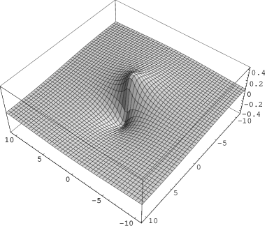
Figure 3: Stress of a screw dislocation near the dislocation line: (a) $\sigma_{xz}$ and (b) $\sigma_{yz}$ are given in units of $\mu b_{z}\kappa/[2\pi]$ .

It is worth to note that the stress (51) agrees with the nonlocal stress given by Eringen [35, 36, 37, 38], with Edelen’s expression [16] and with the stress given by Gutkin and Aifantis [32, 33, 34].

Let us now give some remarks on the double stresses of the screw dislocation. The non-vanishing components are given by (and the components due to the symmetry $\tau_{(ij)k}$)

$$\tau_{zyx}=\frac{1}{\kappa^{2}}\,\partial^{2}_{xx}F,\qquad\tau_{zxy}=-\frac{1}{\kappa^{2}}\,\partial^{2}_{yy}F,\qquad\tau_{zyy}=-\tau_{zxx}=\frac{1}{\kappa^{2}}\,\partial^{2}_{xy}F.$$ (53)

They have a similar form like the elastic bend-twist tensor of a screw dislocation given in [46]. This means that the double stresses are singular at $r=0$. Because the double stress is a simple gradient of the Cauchy stress which is not singular in our case, it is less singular as a gradient of the stress calculated in classical elasticity.

3.2 Edge dislocation: ${\boldsymbol{b}}=(b_{x},0,0)$

In the case of plane strain, we may make the following stress function ansatz

$$\overset{\kern 1.0pt\circ}{\sigma}{}_{ij}=\left(\begin{array}[]{ccc}\partial^{2}_{yy}\overset{\kern 1.0pt\circ}{f}&-\partial^{2}_{xy}\overset{\kern 1.0pt\circ}{f}&0\\ -\partial^{2}_{xy}\overset{\kern 1.0pt\circ}{f}&\partial^{2}_{xx}\overset{\kern 1.0pt\circ}{f}&0\\ 0&0&\nu\Delta\overset{\kern 1.0pt\circ}{f}\end{array}\right),\quad\sigma_{ij}=\left(\begin{array}[]{ccc}\partial^{2}_{yy}f&-\partial^{2}_{xy}f&0\\ -\partial^{2}_{xy}f&\partial^{2}_{xx}f&0\\ 0&0&\nu\Delta f\end{array}\right).$$ (60)

Obviously, it yields $\sigma_{zz}=\nu(\sigma_{xx}+\sigma_{yy})$. For an edge dislocation with Burgers vector $b_{x}$, we use the corresponding Airy’s stress function [23]

$$\overset{\kern 1.0pt\circ}{f}=-\frac{\mu b_{x}}{2\pi(1-\nu)}\,y\ln r.$$ (61)

If we substitute (60) and (61) into (29), we get the inhomogeneous Helmholtz equation for the stress function $f$

$$\Big{(}1-\kappa^{-2}\Delta\Big{)}f=-\frac{\mu b_{x}}{2\pi(1-\nu)}\,y\ln r.$$ (62)

The nonsingular solution for the modified stress function of a straight edge dislocation is given by [19, 46]

$$f=-\frac{\mu b_{x}}{2\pi(1-\nu)}\,y\bigg{\{}\ln r+\frac{2}{\kappa^{2}r^{2}}\Big{(}1-\kappa rK_{1}(\kappa r)\Big{)}\bigg{\}}.$$ (63)

By means of Eqs. (60) and (63), the elastic stress is given as [19]

$$\sigma_{xx}=-\frac{\mu b_{x}}{2\pi(1-\nu)}\,\frac{y}{r^{4}}\bigg{\{}\big{(}y^{2}+3x^{2}\big{)}+\frac{4}{\kappa^{2}r^{2}}\big{(}y^{2}-3x^{2}\big{)}-2y^{2}\kappa rK_{1}(\kappa r)-2\big{(}y^{2}-3x^{2}\big{)}K_{2}(\kappa r)\bigg{\}},$$

$$\sigma_{yy}=-\frac{\mu b_{x}}{2\pi(1-\nu)}\,\frac{y}{r^{4}}\bigg{\{}\big{(}y^{2}-x^{2}\big{)}-\frac{4}{\kappa^{2}r^{2}}\big{(}y^{2}-3x^{2}\big{)}-2x^{2}\kappa rK_{1}(\kappa r)+2\big{(}y^{2}-3x^{2}\big{)}K_{2}(\kappa r)\bigg{\}},$$

$$\sigma_{xy}=\frac{\mu b_{x}}{2\pi(1-\nu)}\,\frac{x}{r^{4}}\bigg{\{}\big{(}x^{2}-y^{2}\big{)}-\frac{4}{\kappa^{2}r^{2}}\big{(}x^{2}-3y^{2}\big{)}-2y^{2}\kappa rK_{1}(\kappa r)+2\big{(}x^{2}-3y^{2}\big{)}K_{2}(\kappa r)\bigg{\}},$$

$$\sigma_{zz}=-\frac{\mu b_{x}\nu}{\pi(1-\nu)}\,\frac{y}{r^{2}}\Big{\{}1-\kappa rK_{1}(\kappa r)\Big{\}}.$$ (64)

The stress (64) is zero at $r=0$. In fact, the “classical” singularities are eliminated due to the behaviour of the Bessel functions at the dislocation line (see Appendix A). The stress (64) has the following extreme values: $|\sigma_{xx}(0,y)|\simeq 0.546\kappa\frac{\mu b_{x}}{2\pi(1-\nu)}$ at $|y|\simeq 0.996\kappa^{-1}$, $|\sigma_{yy}(0,y)|\simeq 0.260\kappa\frac{\mu b_{x}}{2\pi(1-\nu)}$ at $|y|\simeq 1.494\kappa^{-1}$, $|\sigma_{xy}(x,0)|\simeq 0.260\kappa\frac{\mu b_{x}}{2\pi(1-\nu)}$ at $|x|\simeq 1.494\kappa^{-1}$, and $|\sigma_{zz}(0,y)|\simeq 0.399\kappa\frac{\mu b_{x}\nu}{\pi(1-\nu)}$ at $|y|\simeq 1.114\kappa^{-1}$. The stress is plotted in Fig. 4.

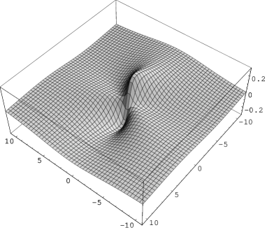
Figure 4: Stress of an edge dislocation: (a) $\sigma_{xx}$, (b) $\sigma_{xy}$, (c) $\sigma_{yy}$ are given in units of $\mu b_{x}\kappa/[2\pi(1-\nu)]$ and (d) $\sigma_{zz}$ is given in units of $\mu b_{x}\nu\kappa/[\pi(1-\nu)]$ .

The corresponding trace of the stress tensor $\sigma_{kk}=\sigma_{xx}+\sigma_{yy}+\sigma_{zz}$ produced by the edge dislocation is

$$\sigma_{kk}=-\frac{\mu b_{x}(1+\nu)}{\pi(1-\nu)}\,\frac{y}{r^{2}}\Big{\{}1-\kappa rK_{1}(\kappa r)\Big{\}}.$$ (65)

Using the inverse of Hooke’s law, we find for the elastic strain of this edge dislocation

$$E_{xx}=-\frac{b_{x}}{4\pi(1-\nu)}\,\frac{y}{r^{2}}\bigg{\{}(1-2\nu)+\frac{2x^{2}}{r^{2}}+\frac{4}{\kappa^{2}r^{4}}\big{(}y^{2}-3x^{2}\big{)}$$

$$\hskip 128.0374pt-2\left(\frac{y^{2}}{r^{2}}-\nu\right)\kappa rK_{1}(\kappa r)-\frac{2}{r^{2}}\big{(}y^{2}-3x^{2}\big{)}K_{2}(\kappa r)\bigg{\}},$$ (66)

$$E_{yy}=-\frac{b_{x}}{4\pi(1-\nu)}\,\frac{y}{r^{2}}\bigg{\{}(1-2\nu)-\frac{2x^{2}}{r^{2}}-\frac{4}{\kappa^{2}r^{4}}\big{(}y^{2}-3x^{2}\big{)}$$

$$\hskip 128.0374pt-2\left(\frac{x^{2}}{r^{2}}-\nu\right)\kappa rK_{1}(\kappa r)+\frac{2}{r^{2}}\big{(}y^{2}-3x^{2}\big{)}K_{2}(\kappa r)\bigg{\}},$$

$$E_{xy}=\frac{b_{x}}{4\pi(1-\nu)}\,\frac{x}{r^{2}}\bigg{\{}1-\frac{2y^{2}}{r^{2}}-\frac{4}{\kappa^{2}r^{4}}\big{(}x^{2}-3y^{2}\big{)}-\frac{2y^{2}}{r^{2}}\,\kappa rK_{1}(\kappa r)+\frac{2}{r^{2}}\big{(}x^{2}-3y^{2}\big{)}K_{2}(\kappa r)\bigg{\}}.$$

The strain (3.2) has the extreme values ($\nu=0.3$): $|E_{xx}(0,y)|\simeq 0.308\kappa\frac{b_{x}}{4\pi(1-\nu)}$ at $|y|\simeq 0.922\kappa^{-1}$, $|E_{yy}(0,y)|\simeq 0.010\kappa\frac{b_{x}}{4\pi(1-\nu)}$ at $|y|\simeq 0.218\kappa^{-1}$, $|E_{yy}(0,y)|\simeq 0.054\kappa\frac{b_{x}}{4\pi(1-\nu)}$ at $|y|\simeq 4.130\kappa^{-1}$, and $|E_{xy}(x,0)|\simeq 0.260\kappa\frac{b_{x}}{4\pi(1-\nu)}$ at $|x|\simeq 1.494\kappa^{-1}$. In addition, it is interesting to note that $E_{yy}(0,y)$ is much smaller than $E_{xx}(0,y)$ within the core region (see also [32]). The dilatation $E_{kk}$ reads

$$E_{kk}=-\frac{b_{x}(1-2\nu)}{2\pi(1-\nu)}\,\frac{y}{r^{2}}\Big{\{}1-\kappa rK_{1}(\kappa r)\Big{\}}.$$ (67)

The strain and the dilatation are zero at the dislocation line.

It is interesting to note that the stress (64) and the strain (3.2) of a dislocation with Burgers vector $b_{x}$ agree with the expressions calculated by Gutkin and Aifantis [32, 33, 34] by using the technique of Fourier transformation.

3.3 Edge dislocation: ${\boldsymbol{b}}=(0,b_{y},0)$

Let us now complete the case of dislocations with the edge dislocation with Burgers vector $b_{y}$. Again it is a plane strain state such that we can use the stress function ansatz (60). But now Airy’s stress function reads

$$\overset{\kern 1.0pt\circ}{f}=\frac{\mu b_{y}}{2\pi(1-\nu)}\,x\ln r.$$ (68)

Substituting (60) and (68) into (29) we find

$$\Big{(}1-\kappa^{-2}\Delta\Big{)}f=\frac{\mu b_{y}}{2\pi(1-\nu)}\,x\ln r.$$ (69)

Its solution is given by

$$f=\frac{\mu b_{y}}{2\pi(1-\nu)}\,x\bigg{\{}\ln r+\frac{2}{\kappa^{2}r^{2}}\Big{(}1-\kappa rK_{1}(\kappa r)\Big{)}\bigg{\}}.$$ (70)

Then we find for the elastic stress

$$\sigma_{xx}=\frac{\mu b_{y}}{2\pi(1-\nu)}\,\frac{x}{r^{4}}\bigg{\{}\big{(}x^{2}-y^{2}\big{)}-\frac{4}{\kappa^{2}r^{2}}\big{(}x^{2}-3y^{2}\big{)}-2y^{2}\kappa rK_{1}(\kappa r)+2\big{(}x^{2}-3y^{2}\big{)}K_{2}(\kappa r)\bigg{\}},$$

$$\sigma_{yy}=\frac{\mu b_{y}}{2\pi(1-\nu)}\,\frac{x}{r^{4}}\bigg{\{}\big{(}x^{2}+3y^{2}\big{)}+\frac{4}{\kappa^{2}r^{2}}\big{(}x^{2}-3y^{2}\big{)}-2x^{2}\kappa rK_{1}(\kappa r)-2\big{(}x^{2}-3y^{2}\big{)}K_{2}(\kappa r)\bigg{\}},$$

$$\sigma_{xy}=\frac{\mu b_{y}}{2\pi(1-\nu)}\,\frac{y}{r^{4}}\bigg{\{}\big{(}x^{2}-y^{2}\big{)}-\frac{4}{\kappa^{2}r^{2}}\big{(}3x^{2}-y^{2}\big{)}+2x^{2}\kappa rK_{1}(\kappa r)+2\big{(}3x^{2}-y^{2}\big{)}K_{2}(\kappa r)\bigg{\}},$$

$$\sigma_{zz}=\frac{\mu b_{y}\nu}{\pi(1-\nu)}\,\frac{x}{r^{2}}\Big{\{}1-\kappa rK_{1}(\kappa r)\Big{\}},$$ (71)

and for the trace of the stress tensor

$$\sigma_{kk}=\frac{\mu b_{y}(1+\nu)}{\pi(1-\nu)}\,\frac{x}{r^{2}}\Big{\{}1-\kappa rK_{1}(\kappa r)\Big{\}}.$$ (72)

The stress (71) has following extreme values: $|\sigma_{yy}(x,0)|\simeq 0.546\kappa\frac{\mu b_{y}}{2\pi(1-\nu)}$ at $|x|\simeq 0.996\kappa^{-1}$, $|\sigma_{xx}(x,0)|\simeq 0.260\kappa\frac{\mu b_{y}}{2\pi(1-\nu)}$ at $|x|\simeq 1.494\kappa^{-1}$, $|\sigma_{xy}(0,y)|\simeq 0.260\kappa\frac{\mu b_{y}}{2\pi(1-\nu)}$ at $|y|\simeq 1.494\kappa^{-1}$, and $|\sigma_{zz}(x,0)|\simeq 0.399\kappa\frac{\mu b_{y}\nu}{\pi(1-\nu)}$ at $|x|\simeq 1.114\kappa^{-1}$.

The elastic strain is given by

$$E_{xx}=\frac{b_{y}}{4\pi(1-\nu)}\,\frac{x}{r^{2}}\bigg{\{}(1-2\nu)-\frac{2y^{2}}{r^{2}}-\frac{4}{\kappa^{2}r^{4}}\big{(}x^{2}-3y^{2}\big{)}$$

$$\hskip 128.0374pt-2\left(\frac{y^{2}}{r^{2}}-\nu\right)\kappa rK_{1}(\kappa r)+\frac{2}{r^{2}}\big{(}x^{2}-3y^{2}\big{)}K_{2}(\kappa r)\bigg{\}},$$ (73)

$$E_{yy}=\frac{b_{y}}{4\pi(1-\nu)}\,\frac{x}{r^{2}}\bigg{\{}(1-2\nu)+\frac{2y^{2}}{r^{2}}+\frac{4}{\kappa^{2}r^{4}}\big{(}x^{2}-3y^{2}\big{)}$$

$$\hskip 128.0374pt-2\left(\frac{x^{2}}{r^{2}}-\nu\right)\kappa rK_{1}(\kappa r)-\frac{2}{r^{2}}\big{(}x^{2}-3y^{2}\big{)}K_{2}(\kappa r)\bigg{\}},$$

$$E_{xy}=-\frac{b_{y}}{4\pi(1-\nu)}\,\frac{y}{r^{2}}\bigg{\{}1-\frac{2x^{2}}{r^{2}}+\frac{4}{\kappa^{2}r^{4}}\big{(}3x^{2}-y^{2}\big{)}-\frac{2x^{2}}{r^{2}}\,\kappa rK_{1}(\kappa r)-\frac{2}{r^{2}}\big{(}3x^{2}-y^{2}\big{)}K_{2}(\kappa r)\bigg{\}},$$

and the dilatation reads

$$E_{kk}=\frac{b_{y}(1-2\nu)}{2\pi(1-\nu)}\,\frac{x}{r^{2}}\Big{\{}1-\kappa rK_{1}(\kappa r)\Big{\}}.$$ (74)

The strain (3.3) has the extreme values ($\nu=0.3$): $|E_{yy}(x,0)|\simeq 0.308\kappa\frac{b_{y}}{4\pi(1-\nu)}$ at $|x|\simeq 0.922\kappa^{-1}$, $|E_{xx}(x,0)|\simeq 0.010\kappa\frac{b_{y}}{4\pi(1-\nu)}$ at $|x|\simeq 0.218\kappa^{-1}$, $|E_{xx}(x,0)|\simeq 0.054\kappa\frac{b_{y}}{4\pi(1-\nu)}$ at $|x|\simeq 4.130\kappa^{-1}$, and $|E_{xy}(0,y)|\simeq 0.260\kappa\frac{b_{y}}{4\pi(1-\nu)}$ at $|y|\simeq 1.494\kappa^{-1}$. Again, it is interesting to note that $E_{xx}(x,0)$ is much smaller than $E_{yy}(x,0)$ within the core region. In addition, the stress and strain fields are zero at $r=0$.

In principle, we could calculate the double stresses of edge dislocations. But we do not want to do this in detail. Using Eqs. (64) and (71) we would obtain expressions which are similar in form to the double stresses of the screw dislocation. Again, the double stresses are still singular at the dislocation line. The double stresses  of an edge dislocation are given in terms of the stress function $f$ as derivatives of the third order according to:

$$\tau_{yyx}=\frac{1}{\kappa^{2}}\,\partial^{3}_{xxx}f,\qquad\qquad\tau_{yyy}=-\tau_{xyx}=\frac{1}{\kappa^{2}}\,\partial^{3}_{xxy}f$$

$$\tau_{xxy}=\frac{1}{\kappa^{2}}\,\partial^{3}_{yyy}f,\qquad\qquad\tau_{xxx}=-\tau_{xyy}=\frac{1}{\kappa^{2}}\,\partial^{3}_{yyx}f$$

$$\tau_{zzx}=\nu(\tau_{xxx}+\tau_{yyx})\qquad\tau_{zzy}=\nu(\tau_{xxy}+\tau_{yyy})\,.$$ (75)

They are singular at $r=0$.

4 Disclinations

In this section we consider straight disclinations in an infinitely extended medium. The disclination line coincides with the $z$-axis of a Cartesian coordinate system. We are using deWit’s expressions [14] for the classical stress and strain fields (see also [48]).

4.1 Wedge disclination: $\boldsymbol{\Omega}=(0,0,\Omega_{z})$

As in the case of edge dislocations we may use the stress function ansatz (60) for the wedge disclination as well. It is obvious because the wedge disclination corresponds also to plane strain. Using the stress function of a “classical” wedge disclination,

$$\overset{\kern 1.0pt\circ}{f}=\frac{\mu\Omega_{z}}{4\pi(1-\nu)}\,r^{2}\left\{\ln r-\frac{1-4\nu}{2(1-2\nu)}\right\},$$ (76)

and (60), we obtain the following equation which gives the solution of a “modified” stress function of a wedge disclination

$$\Big{(}1-\kappa^{-2}\Delta\Big{)}f=\frac{\mu\Omega_{z}}{4\pi(1-\nu)}\,r^{2}\left(\ln r-\frac{1-4\nu}{2(1-2\nu)}\right).$$ (77)

Consequently, the “modified” stress function of a wedge disclination is given by (see also [49])

$$f=\frac{\mu\Omega_{z}}{4\pi(1-\nu)}\left\{r^{2}\bigg{(}\ln r-\frac{1-4\nu}{2(1-2\nu)}\bigg{)}+\frac{4}{\kappa^{2}}\,\bigg{(}\ln r+K_{0}(\kappa r)+\frac{1}{2(1-2\nu)}\bigg{)}\right\}.$$ (78)

Substituting (78) into (60), we find for the stresses of a wedge disclination

$$\sigma_{xx}=\frac{\mu\Omega_{z}}{2\pi(1-\nu)}\,\bigg{\{}\ln r+\frac{y^{2}}{r^{2}}+\frac{\nu}{1-2\nu}+K_{0}(\kappa r)+\frac{\big{(}x^{2}-y^{2}\big{)}}{\kappa^{2}r^{4}}\Big{(}2-\kappa^{2}r^{2}K_{2}(\kappa r)\Big{)}\bigg{\}},$$

$$\sigma_{yy}=\frac{\mu\Omega_{z}}{2\pi(1-\nu)}\,\bigg{\{}\ln r+\frac{x^{2}}{r^{2}}+\frac{\nu}{1-2\nu}+K_{0}(\kappa r)-\frac{\big{(}x^{2}-y^{2}\big{)}}{\kappa^{2}r^{4}}\Big{(}2-\kappa^{2}r^{2}K_{2}(\kappa r)\Big{)}\bigg{\}},$$

$$\sigma_{xy}=-\frac{\mu\Omega_{z}}{2\pi(1-\nu)}\,\frac{xy}{r^{2}}\bigg{\{}1-\frac{2}{\kappa^{2}r^{2}}\Big{(}2-\kappa^{2}r^{2}K_{2}(\kappa r)\Big{)}\bigg{\}},$$

$$\sigma_{zz}=\frac{\mu\Omega_{z}\,\nu}{\pi(1-\nu)}\,\bigg{\{}\ln r+\frac{1}{2(1-2\nu)}+K_{0}(\kappa r)\bigg{\}},$$ (79)

and for the trace of the stress tensor

$$\sigma_{kk}=\frac{\mu\Omega_{z}(1+\nu)}{\pi(1-\nu)}\,\bigg{\{}\ln r+\frac{1}{2(1-2\nu)}+K_{0}(\kappa r)\bigg{\}}.$$ (80)

The stress is plotted in Fig. 5.

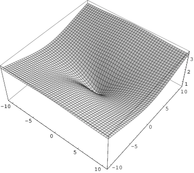
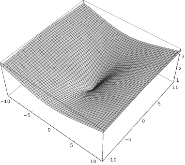
Figure 5: Stress of a wedge disclination: (a) $\sigma_{xx}$, (b) $\sigma_{xy}$, (c) $\sigma_{yy}$ are given in units of $\mu\Omega_{z}/[2\pi(1-\nu)]$ and (d) $\sigma_{zz}$ is given in units of $\mu\Omega_{z}\nu/[\pi(1-\nu)]$ .

Using Eqs. (A.1) and (A.3), we obtain for the stress at $r=0$

$$\sigma_{xx}(0)=\sigma_{yy}(0)=\frac{\mu\Omega_{z}}{2\pi(1-\nu)}\,\bigg{\{}\frac{\nu}{1-2\nu}-\gamma-\ln\frac{\kappa}{2}+\frac{1}{2}\bigg{\}},\quad\sigma_{xy}(0)=0,$$

$$\sigma_{zz}(0)=\frac{\nu}{1+\nu}\sigma_{kk}(0)=\frac{\mu\Omega_{z}\nu}{\pi(1-\nu)}\,\bigg{\{}\frac{\nu}{1-2\nu}-\gamma-\ln\frac{\kappa}{2}\bigg{\}}.$$

Consequently, the stress is finite at the disclination line in contrast to the unphysical stress singularity in “classical” disclination theory. The elastic strain is easily calculated as

$$E_{xx}=\frac{\Omega_{z}}{4\pi(1-\nu)}\bigg{\{}(1-2\nu)\big{(}\ln r+K_{0}(\kappa r)\big{)}+\frac{y^{2}}{r^{2}}+\frac{(x^{2}-y^{2})}{\kappa^{2}r^{4}}\Big{(}2-\kappa^{2}r^{2}K_{2}(\kappa r)\Big{)}\bigg{\}},$$

$$E_{yy}=\frac{\Omega_{z}}{4\pi(1-\nu)}\bigg{\{}(1-2\nu)\big{(}\ln r+K_{0}(\kappa r)\big{)}+\frac{x^{2}}{r^{2}}-\frac{(x^{2}-y^{2})}{\kappa^{2}r^{4}}\Big{(}2-\kappa^{2}r^{2}K_{2}(\kappa r)\Big{)}\bigg{\}},$$

$$E_{xy}=-\frac{\Omega_{z}}{4\pi(1-\nu)}\,\frac{xy}{r^{2}}\bigg{\{}1-\frac{2}{\kappa^{2}r^{2}}\Big{(}2-\kappa^{2}r^{2}K_{2}(\kappa r)\Big{)}\bigg{\}},$$ (81)

and for the dilatation we obtain

$$E_{kk}=\frac{\Omega_{z}}{2\pi(1-\nu)}\bigg{\{}(1-2\nu)\big{(}\ln r+K_{0}(\kappa r)\big{)}+\frac{1}{2}\bigg{\}}.$$ (82)

Again using Eqs. (A.1) and (A.3) the strain reads at $r=0$

$$E_{xx}(0)=E_{yy}(0)=\frac{1}{2}E_{kk}(0)=-\frac{\Omega_{z}}{4\pi(1-\nu)}\,\bigg{\{}(1-2\nu)\Big{(}\gamma+\ln\frac{\kappa}{2}\Big{)}-\frac{1}{2}\bigg{\}},\quad E_{xy}(0)=0.$$

Now we calculate the non-vanishing components of the double stress for the wedge disclination. They are given in terms of the stress function as follows

$$\tau_{yyx}=\frac{1}{\kappa^{2}}\,\partial^{3}_{xxx}f,\qquad\tau_{xxy}=\frac{1}{\kappa^{2}}\,\partial^{3}_{yyy}f,\qquad\tau_{yyy}=-\tau_{xyx}=\frac{1}{\kappa^{2}}\,\partial^{3}_{yxx}f,$$

$$\tau_{xxx}=-\tau_{xyy}=\frac{1}{\kappa^{2}}\,\partial^{3}_{xyy}f,\qquad\tau_{zzx}=\frac{\nu}{\kappa^{2}}\,\partial_{x}\Delta f,\qquad\tau_{zzy}=\frac{\nu}{\kappa^{2}}\,\partial_{y}\Delta f.$$ (83)

So we obtain for the double stresses of the wedge disclination

$$\tau_{yyx}=\frac{\mu\Omega_{z}}{2\pi(1-\nu)\kappa^{2}}\,\frac{x}{r^{4}}\bigg{\{}\big{(}x^{2}+3y^{2}\big{)}+\frac{4}{\kappa^{2}r^{2}}\big{(}x^{2}-3y^{2}\big{)}-2x^{2}\kappa rK_{1}(\kappa r)-2\big{(}x^{2}-3y^{2}\big{)}K_{2}(\kappa r)\bigg{\}},$$

$$\tau_{xxy}=\frac{\mu\Omega_{z}}{2\pi(1-\nu)\kappa^{2}}\,\frac{y}{r^{4}}\bigg{\{}\big{(}y^{2}+3x^{2}\big{)}+\frac{4}{\kappa^{2}r^{2}}\big{(}y^{2}-3x^{2}\big{)}-2y^{2}\kappa rK_{1}(\kappa r)-2\big{(}y^{2}-3x^{2}\big{)}K_{2}(\kappa r)\bigg{\}},$$

$$\tau_{yyy}=\frac{\mu\Omega_{z}}{2\pi(1-\nu)\kappa^{2}}\,\frac{y}{r^{4}}\bigg{\{}\big{(}y^{2}-x^{2}\big{)}-\frac{4}{\kappa^{2}r^{2}}\big{(}y^{2}-3x^{2}\big{)}-2x^{2}\kappa rK_{1}(\kappa r)+2\big{(}y^{2}-3x^{2}\big{)}K_{2}(\kappa r)\bigg{\}},$$

$$\tau_{xxx}=\frac{\mu\Omega_{z}}{2\pi(1-\nu)\kappa^{2}}\,\frac{x}{r^{4}}\bigg{\{}\big{(}x^{2}-y^{2}\big{)}-\frac{4}{\kappa^{2}r^{2}}\big{(}x^{2}-3y^{2}\big{)}-2y^{2}\kappa rK_{1}(\kappa r)+2\big{(}x^{2}-3y^{2}\big{)}K_{2}(\kappa r)\bigg{\}},$$

$$\tau_{zzx}=\frac{\mu\Omega_{z}\nu}{\pi(1-\nu)\kappa^{2}}\,\frac{x}{r^{2}}\Big{\{}1-\kappa rK_{1}(\kappa r)\Big{\}},$$

$$\tau_{zzy}=\frac{\mu\Omega_{z}\nu}{\pi(1-\nu)\kappa^{2}}\,\frac{y}{r^{2}}\Big{\{}1-\kappa rK_{1}(\kappa r)\Big{\}}.$$ (84)

This double stress tensor has some interesting features. First, it is not singular. Second, it has a similar form like the stress field of an edge dislocation (compare with Eqs. (64) and (71)). Thus, the components are zero at $r=0$ and have extremum values near the disclination line.

4.2 Twist disclination: $\boldsymbol{\Omega}=(\Omega_{x},0,0)$

In the case of twist disclination the problem, which we want to consider, is more complicated than those of dislocations and of the wedge disclination. The reason is that the situation is no longer a proper two-dimensional problem. In the case of twist disclination the three-dimensional space may be considered as a product of the two-dimensional $xy$-plane and the independent one-dimensional $z$-line [14]. Thus, the $z$-axis plays a peculiar role.

First, we make an ansatz which fulfills the stress equilibrium. It is given by

$$\overset{\kern 1.0pt\circ}{\sigma}{}_{ij} =\left(\begin{array}[]{ccc}\ \,\partial^{2}_{yy}\overset{\kern 1.0pt\circ}{f}&-\partial^{2}_{xy}\overset{\kern 1.0pt\circ}{f}&-\partial_{y}\overset{\kern 1.0pt\circ}{F}+\partial_{z}\overset{\kern 1.0pt\circ}{g}\\ -\partial^{2}_{xy}\overset{\kern 1.0pt\circ}{f}&\partial^{2}_{xx}\overset{\kern 1.0pt\circ}{f}&\partial_{x}\overset{\kern 1.0pt\circ}{F}\\ -\partial_{y}\overset{\kern 1.0pt\circ}{F}+\partial_{z}\overset{\kern 1.0pt\circ}{g}&\partial_{x}\overset{\kern 1.0pt\circ}{F}&\overset{\kern 1.0pt\circ}{p}\end{array}\right),\$$ (88)

$$\sigma_{ij} =\left(\begin{array}[]{ccc}\ \,\partial^{2}_{yy}f&-\partial^{2}_{xy}f&-\partial_{y}F+\partial_{z}g\\ -\partial^{2}_{xy}f&\partial^{2}_{xx}f&\partial_{x}F\\ -\partial_{y}F+\partial_{z}g&\partial_{x}F&p\end{array}\right),$$ (92)

with the relations

$$\overset{\kern 1.0pt\circ}{p}=\nu\Delta\overset{\kern 1.0pt\circ}{f}=-\partial_{x}\overset{\kern 1.0pt\circ}{g},\qquad p=\nu\Delta f=-\partial_{x}g,$$ (93)

which follow from $\partial_{i}\overset{\kern 1.0pt\circ}{\sigma}_{zi}=0$ and $\partial_{i}\sigma_{zi}=0$. One can see the special role of $z$ in the ansatz (88). The ansatz (88) is not only an addition of the anti-plane (47) and plane strain (60) situation because an additional stress function $\overset{\kern 1.0pt\circ}{g}$ or $g$ enters the ansatz. The following “classical” stress functions,

$$\overset{\kern 1.0pt\circ}{f}=-\frac{\mu\Omega_{x}}{2\pi(1-\nu)}\,zx\ln r,$$

$$\overset{\kern 1.0pt\circ}{F}=\frac{\mu\Omega_{x}}{2\pi(1-\nu)}\,y\ln r,$$

$$\overset{\kern 1.0pt\circ}{g}=\frac{\mu\Omega_{x}\nu}{\pi(1-\nu)}\,z\ln r,$$ (94)

may be used to reproduce deWit’s expressions for the stress and strain fields of the twist disclination. Substituting (4.2) and (88) into (29), the following Helmholtz equations to determine the “modified” stress functions follow

$$\Big{(}1-\kappa^{-2}\Delta\Big{)}f =-\frac{\mu\Omega_{x}}{2\pi(1-\nu)}\,zx\ln r,$$

$$\Big{(}1-\kappa^{-2}\Delta\Big{)}F =\frac{\mu\Omega_{x}}{2\pi(1-\nu)}\,x\ln r,$$

$$\Big{(}1-\kappa^{-2}\Delta\Big{)}g =\frac{\mu\Omega_{x}\nu}{\pi(1-\nu)}\,z\ln r.$$ (95)

The solutions of the modified stress functions are given by

$$f =-\frac{\mu\Omega_{x}}{2\pi(1-\nu)}\,zx\bigg{\{}\ln r+\frac{2}{\kappa^{2}r^{2}}\Big{(}1-\kappa rK_{1}(\kappa r)\Big{)}\bigg{\}},$$

$$F =\frac{\mu\Omega_{x}}{2\pi(1-\nu)}\,y\bigg{\{}\ln r+\frac{2}{\kappa^{2}r^{2}}\Big{(}1-\kappa rK_{1}(\kappa r)\Big{)}\bigg{\}},$$

$$g =\frac{\mu\Omega_{x}\nu}{\pi(1-\nu)}\,z\Big{\{}\ln r+K_{0}(\kappa r)\Big{\}},$$ (96)

By means of (88) and (4.2) we are able to calculate the stress

$$\sigma_{xx}=-\frac{\mu\Omega_{x}}{2\pi(1-\nu)}\,\frac{zx}{r^{4}}\bigg{\{}\big{(}x^{2}-y^{2}\big{)}-\frac{4}{\kappa^{2}r^{2}}\big{(}x^{2}-3y^{2}\big{)}-2y^{2}\kappa rK_{1}(\kappa r)+2\big{(}x^{2}-3y^{2}\big{)}K_{2}(\kappa r)\bigg{\}},$$

$$\sigma_{yy}=-\frac{\mu\Omega_{x}}{2\pi(1-\nu)}\,\frac{zx}{r^{4}}\bigg{\{}\big{(}x^{2}+3y^{2}\big{)}+\frac{4}{\kappa^{2}r^{2}}\big{(}x^{2}-3y^{2}\big{)}-2x^{2}\kappa rK_{1}(\kappa r)-2\big{(}x^{2}-3y^{2}\big{)}K_{2}(\kappa r)\bigg{\}},$$

$$\sigma_{xy}=-\frac{\mu\Omega_{x}}{2\pi(1-\nu)}\,\frac{zy}{r^{4}}\bigg{\{}\big{(}x^{2}-y^{2}\big{)}-\frac{4}{\kappa^{2}r^{2}}\big{(}3x^{2}-y^{2}\big{)}+2x^{2}\kappa rK_{1}(\kappa r)+2\big{(}3x^{2}-y^{2}\big{)}K_{2}(\kappa r)\bigg{\}},$$

$$\sigma_{zz}=-\frac{\mu\Omega_{x}\nu}{\pi(1-\nu)}\,\frac{zx}{r^{2}}\Big{\{}1-\kappa rK_{1}(\kappa r)\Big{\}},$$

$$\sigma_{zx}=-\frac{\mu\Omega_{x}}{2\pi(1-\nu)}\,\bigg{\{}(1-2\nu)\big{(}\ln r+K_{0}(\kappa r)\big{)}+\frac{y^{2}}{r^{2}}+\frac{\big{(}x^{2}-y^{2}\big{)}}{\kappa^{2}r^{4}}\Big{(}2-\kappa^{2}r^{2}K_{2}(\kappa r)\Big{)}\bigg{\}},$$

$$\sigma_{zy}=\frac{\mu\Omega_{x}}{2\pi(1-\nu)}\,\frac{xy}{r^{2}}\bigg{\{}1-\frac{2}{\kappa^{2}r^{2}}\Big{(}2-\kappa^{2}r^{2}K_{2}(\kappa r)\Big{)}\bigg{\}}.$$ (97)

The trace of the stress tensor reads in this case

$$\sigma_{kk}=-\frac{\mu\Omega_{x}(1+\nu)}{\pi(1-\nu)}\,\frac{zx}{r^{2}}\Big{\{}1-\kappa rK_{1}(\kappa r)\Big{\}}.$$ (98)

The stress (4.2) has its extreme values in the $xy$-plane: $|\sigma_{yy}(x,0)|\simeq 0.546\kappa\frac{\mu\Omega_{x}z}{2\pi(1-\nu)}$ at $|x|\simeq 0.996\kappa^{-1}$, $|\sigma_{xx}(x,0)|\simeq 0.260\kappa\frac{\mu\Omega_{x}z}{2\pi(1-\nu)}$ at $|x|\simeq 1.494\kappa^{-1}$, $|\sigma_{xy}(0,y)|\simeq 0.260\kappa\frac{\mu\Omega_{x}z}{2\pi(1-\nu)}$ at $|y|\simeq 1.494\kappa^{-1}$, and $|\sigma_{zz}(x,0)|\simeq 0.399\kappa\frac{\mu\Omega_{x}z\nu}{\pi(1-\nu)}$ at $|x|\simeq 1.114\kappa^{-1}$. The stress $\sigma_{zx}$ has at $r=0$ the value: $\sigma_{zx}(0)\simeq\frac{\mu\Omega_{x}}{2\pi(1-\nu)}[(1-2\nu)(\gamma+\ln\frac{\kappa}{2})-0.5]$ and with $\nu=0.3$: $\sigma_{zx}(0)\simeq\frac{\mu\Omega_{x}}{2\pi(1-\nu)}[0.4\ln\kappa-0.546]$.

The corresponding elastic strain is given by

$$E_{xx}=-\frac{\Omega_{x}}{4\pi(1-\nu)}\,\frac{zx}{r^{2}}\bigg{\{}(1-2\nu)-\frac{2y^{2}}{r^{2}}-\frac{4}{\kappa^{2}r^{4}}\big{(}x^{2}-3y^{2}\big{)}$$

$$\hskip 142.26378pt-2\left(\frac{y^{2}}{r^{2}}-\nu\right)\kappa rK_{1}(\kappa r)+\frac{2}{r^{2}}\big{(}x^{2}-3y^{2}\big{)}K_{2}(\kappa r)\bigg{\}},$$

$$E_{yy}=-\frac{\Omega_{x}}{4\pi(1-\nu)}\,\frac{zx}{r^{2}}\bigg{\{}(1-2\nu)+\frac{2y^{2}}{r^{2}}+\frac{4}{\kappa^{2}r^{4}}\big{(}x^{2}-3y^{2}\big{)}$$

$$\hskip 142.26378pt-2\left(\frac{x^{2}}{r^{2}}-\nu\right)\kappa rK_{1}(\kappa r)-\frac{2}{r^{2}}\big{(}x^{2}-3y^{2}\big{)}K_{2}(\kappa r)\bigg{\}},$$

$$E_{xy}=\frac{\Omega_{x}}{4\pi(1-\nu)}\,\frac{zy}{r^{2}}\bigg{\{}1-\frac{2x^{2}}{r^{2}}+\frac{4}{\kappa^{2}r^{4}}\big{(}3x^{2}-y^{2}\big{)}-\frac{2x^{2}}{r^{2}}\,\kappa rK_{1}(\kappa r)-\frac{2}{r^{2}}\big{(}3x^{2}-y^{2}\big{)}K_{2}(\kappa r)\bigg{\}},$$

$$E_{zx}=-\frac{\Omega_{x}}{4\pi(1-\nu)}\,\bigg{\{}(1-2\nu)\big{(}\ln r+K_{0}(\kappa r)\big{)}+\frac{y^{2}}{r^{2}}+\frac{\big{(}x^{2}-y^{2}\big{)}}{\kappa^{2}r^{4}}\Big{(}2-\kappa^{2}r^{2}K_{2}(\kappa r)\Big{)}\bigg{\}},$$

$$E_{zy}=\frac{\Omega_{x}}{4\pi(1-\nu)}\,\frac{xy}{r^{2}}\bigg{\{}1-\frac{2}{\kappa^{2}r^{2}}\Big{(}2-\kappa^{2}r^{2}K_{2}(\kappa r)\Big{)}\bigg{\}}.$$ (99)

The dilatation reads

$$E_{kk}=-\frac{\Omega_{x}(1-2\nu)}{2\pi(1-\nu)}\,\frac{zx}{r^{2}}\Big{\{}1-\kappa rK_{1}(\kappa r)\Big{\}}.$$ (100)

The strain (4.2) has the extreme values ($\nu=0.3$): $|E_{yy}(x,0)|\simeq 0.308\kappa\frac{\Omega_{x}z}{4\pi(1-\nu)}$ at $|x|\simeq 0.922\kappa^{-1}$, $|E_{xx}(x,0)|\simeq 0.010\kappa\frac{\Omega_{x}z}{4\pi(1-\nu)}$ at $|x|\simeq 0.218\kappa^{-1}$, $|E_{xx}(x,0)|\simeq 0.054\kappa\frac{\Omega_{x}z}{4\pi(1-\nu)}$ at $|x|\simeq 4.130\kappa^{-1}$, and $|E_{xy}(0,y)|\simeq 0.260\kappa\frac{\Omega_{x}z}{4\pi(1-\nu)}$ at $|y|\simeq 1.494\kappa^{-1}$. Again, it is interesting to note that $E_{xx}(x,0)$ is much smaller than $E_{yy}(x,0)$ within the core region. The strain $E_{zx}$ has at $r=0$ the value: $E_{zy}(0)\simeq\frac{\mu\Omega_{x}}{4\pi(1-\nu)}[(1-2\nu)(\gamma+\ln\frac{\kappa}{2})-0.5]$. The dilatation has its extremum $|E_{kk}(x,0)|\simeq 0.399\kappa\frac{\Omega_{x}(1-2\nu)z}{2\pi(1-\nu)}$ at $|x|\simeq 1.114\kappa^{-1}$.

It is interesting to note that there is a relation between the stress and strain fields of twist disclinations and edge disclinations. If one replaces $\Omega_{x}z$ by $-b_{y}$ in the components of the stress $\sigma_{xx}$ – $\sigma_{zz}$ in (4.2) and in the strain $E_{xx}$ – $E_{xy}$ in (4.2), the stress (71) and the strain (3.3) are obtained.

4.3 Twist disclination: $\boldsymbol{\Omega}=(0,\Omega_{y},0)$

For the twist disclination with Frank vector $\Omega_{y}$ we make a similar ansatz like the ansatz (88) of the twist disclination with Frank vector $\Omega_{x}$. It is given by

$$\overset{\kern 1.0pt\circ}{\sigma}{}_{ij}=\left(\begin{array}[]{ccc}\ \,\partial^{2}_{yy}\overset{\kern 1.0pt\circ}{f}&-\partial^{2}_{xy}\overset{\kern 1.0pt\circ}{f}&-\partial_{y}\overset{\kern 1.0pt\circ}{F}\\ -\partial^{2}_{xy}\overset{\kern 1.0pt\circ}{f}&\partial^{2}_{xx}\overset{\kern 1.0pt\circ}{f}&\partial_{x}\overset{\kern 1.0pt\circ}{F}+\partial_{z}\overset{\kern 1.0pt\circ}{g}\\ -\partial_{y}\overset{\kern 1.0pt\circ}{F}&\partial_{x}\overset{\kern 1.0pt\circ}{F}+\partial_{z}\overset{\kern 1.0pt\circ}{g}&\overset{\kern 1.0pt\circ}{p}\end{array}\right),\quad\sigma_{ij}=\left(\begin{array}[]{ccc}\ \,\partial^{2}_{yy}f&-\partial^{2}_{xy}f&-\partial_{y}F\\ -\partial^{2}_{xy}f&\partial^{2}_{xx}f&\partial_{x}F+\partial_{z}g\\ -\partial_{y}F&\partial_{x}F+\partial_{z}g&p\end{array}\right),$$ (107)

with the relations

$$\overset{\kern 1.0pt\circ}{p}=\nu\Delta\overset{\kern 1.0pt\circ}{f}=-\partial_{y}\overset{\kern 1.0pt\circ}{g},\qquad p=\nu\Delta f=-\partial_{y}g,$$ (108)

which follow again from $\partial_{i}\overset{\kern 1.0pt\circ}{\sigma}_{zi}=0$ and $\partial_{i}\sigma_{zi}=0$. The only one difference between (88) and (107) is the position of the stress function $g$. In the present case, the “classical” stress functions are given by

$$\overset{\kern 1.0pt\circ}{f}=-\frac{\mu\Omega_{y}}{2\pi(1-\nu)}\,zy\ln r,$$

$$\overset{\kern 1.0pt\circ}{F}=-\frac{\mu\Omega_{y}}{2\pi(1-\nu)}\,x\ln r,$$

$$\overset{\kern 1.0pt\circ}{g}=\frac{\mu\Omega_{y}\nu}{\pi(1-\nu)}\,z\ln r.$$ (109)

These three stress functions reproduce the stress and strain fields given by deWit [14]. If we substitute (107) and (4.3) into (29), we get the following inhomogeneous Helmholtz equations

$$\Big{(}1-\kappa^{-2}\Delta\Big{)}f =-\frac{\mu\Omega_{y}x}{2\pi(1-\nu)}\,zy\ln r,$$

$$\Big{(}1-\kappa^{-2}\Delta\Big{)}F =-\frac{\mu\Omega_{y}}{2\pi(1-\nu)}\,x\ln r,$$

$$\Big{(}1-\kappa^{-2}\Delta\Big{)}g =\frac{\mu\Omega_{y}\nu}{\pi(1-\nu)}\,z\ln r.$$ (110)

The solutions of the “modified” stress functions reads now (see also [50])

$$f =-\frac{\mu\Omega_{y}}{2\pi(1-\nu)}\,zy\bigg{\{}\ln r+\frac{2}{\kappa^{2}r^{2}}\Big{(}1-\kappa rK_{1}(\kappa r)\Big{)}\bigg{\}},$$

$$F =-\frac{\mu\Omega_{y}}{2\pi(1-\nu)}\,x\bigg{\{}\ln r+\frac{2}{\kappa^{2}r^{2}}\Big{(}1-\kappa rK_{1}(\kappa r)\Big{)}\bigg{\}},$$

$$g =\frac{\mu\Omega_{y}\nu}{\pi(1-\nu)}\,z\Big{\{}\ln r+K_{0}(\kappa r)\Big{\}}.$$ (111)

So we find for the elastic stress of this disclination [50]

$$\sigma_{xx}=-\frac{\mu\Omega_{y}}{2\pi(1-\nu)}\,\frac{zy}{r^{4}}\bigg{\{}\big{(}y^{2}+3x^{2}\big{)}+\frac{4}{\kappa^{2}r^{2}}\big{(}y^{2}-3x^{2}\big{)}-2y^{2}\kappa rK_{1}(\kappa r)-2\big{(}y^{2}-3x^{2}\big{)}K_{2}(\kappa r)\bigg{\}},$$

$$\sigma_{yy}=-\frac{\mu\Omega_{y}}{2\pi(1-\nu)}\,\frac{zy}{r^{4}}\bigg{\{}\big{(}y^{2}-x^{2}\big{)}-\frac{4}{\kappa^{2}r^{2}}\big{(}y^{2}-3x^{2}\big{)}-2x^{2}\kappa rK_{1}(\kappa r)+2\big{(}y^{2}-3x^{2}\big{)}K_{2}(\kappa r)\bigg{\}},$$

$$\sigma_{xy}=\frac{\mu\Omega_{y}}{2\pi(1-\nu)}\,\frac{zx}{r^{4}}\bigg{\{}\big{(}x^{2}-y^{2}\big{)}-\frac{4}{\kappa^{2}r^{2}}\big{(}x^{2}-3y^{2}\big{)}-2y^{2}\kappa rK_{1}(\kappa r)+2\big{(}x^{2}-3y^{2}\big{)}K_{2}(\kappa r)\bigg{\}},$$

$$\sigma_{zz}=-\frac{\mu\Omega_{y}\nu}{\pi(1-\nu)}\,\frac{zy}{r^{2}}\Big{\{}1-\kappa rK_{1}(\kappa r)\Big{\}},$$

$$\sigma_{zx}=\frac{\mu\Omega_{y}}{2\pi(1-\nu)}\,\frac{xy}{r^{2}}\bigg{\{}1-\frac{2}{\kappa^{2}r^{2}}\Big{(}2-\kappa^{2}r^{2}K_{2}(\kappa r)\Big{)}\bigg{\}},$$

$$\sigma_{zy}=-\frac{\mu\Omega_{y}}{2\pi(1-\nu)}\,\bigg{\{}(1-2\nu)\big{(}\ln r+K_{0}(\kappa r)\big{)}+\frac{x^{2}}{r^{2}}-\frac{\big{(}x^{2}-y^{2}\big{)}}{\kappa^{2}r^{4}}\Big{(}2-\kappa^{2}r^{2}K_{2}(\kappa r)\Big{)}\bigg{\}},$$ (112)

and its trace is given by

$$\sigma_{kk}=-\frac{\mu\Omega_{y}(1+\nu)}{\pi(1-\nu)}\,\frac{zy}{r^{2}}\Big{\{}1-\kappa rK_{1}(\kappa r)\Big{\}}.$$ (113)

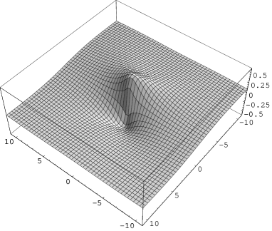
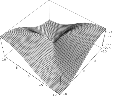
Figure 6: Stress of a twist disclination: (a) $\sigma_{xx}$, (b) $\sigma_{xy}$, (c) $\sigma_{yy}$ are given in units of $\mu\Omega_{y}\kappa z/[2\pi(1-\nu)]$, (d) $\sigma_{zz}$ is given in units of $\mu\Omega_{y}\nu\kappa z/[\pi(1-\nu)]$, (e) $\sigma_{zx}$ and (f) $\sigma_{zy}$ are given in units of $\mu\Omega_{y}/[2\pi(1-\nu)]$ .

It can be seen that the stresses have the following extreme values in the $xy$-plane: $|\sigma_{xx}(0,y)|\simeq 0.546\kappa\frac{\mu\Omega_{y}z}{2\pi(1-\nu)}$ at $|y|\simeq 0.996\kappa^{-1}$, $|\sigma_{yy}(0,y)|\simeq 0.260\kappa\frac{\mu\Omega_{y}z}{2\pi(1-\nu)}$ at $|y|\simeq 1.494\kappa^{-1}$, $|\sigma_{xy}(x,0)|\simeq 0.260\kappa\frac{\mu\Omega_{y}z}{2\pi(1-\nu)}$ at $|x|\simeq 1.494\kappa^{-1}$, $|\sigma_{zz}(0,y)|\simeq 0.399\kappa\frac{\mu\Omega_{y}\nu z}{\pi(1-\nu)}$ at $|y|\simeq 1.114\kappa^{-1}$ and $|\sigma_{kk}(0,y)|\simeq 0.399\kappa\frac{\mu\Omega_{y}(1+\nu)z}{\pi(1-\nu)}$ at $|y|\simeq 1.114\kappa^{-1}$. The stresses $\sigma_{xx}$, $\sigma_{yy}$ and $\sigma_{xy}$ are modified near the disclination core ($0\leq r\leq 12\kappa^{-1}$). The stress $\sigma_{zz}$ and the trace $\sigma_{kk}$ are modified in the region: $0\leq r\leq 6\kappa^{-1}$. Far from the disclination line ($r\gg 12\kappa^{-1}$) the modified and the classical solutions of the stress of a twist disclination coincide. In addition, it can be seen that at $z=0$ the stresses $\sigma_{xx}$ – $\sigma_{zz}$ are zero. The stress $\sigma_{zy}$ has at $r=0$ the value: $\sigma_{zy}(0)\simeq\frac{\mu\Omega_{y}}{2\pi(1-\nu)}[(1-2\nu)(\gamma+\ln\frac{\kappa}{2})-0.5]$ and with $\nu=0.3$: $\sigma_{zy}(0)\simeq\frac{\mu\Omega_{y}}{2\pi(1-\nu)}[0.4\ln\kappa-0.546]$. The stress is plotted in Fig. 6.

For the elastic strain we obtain

$$E_{xx}=-\frac{\Omega_{y}}{4\pi(1-\nu)}\,\frac{zy}{r^{2}}\bigg{\{}(1-2\nu)+\frac{2x^{2}}{r^{2}}+\frac{4}{\kappa^{2}r^{4}}\big{(}y^{2}-3x^{2}\big{)}$$

$$\hskip 142.26378pt-2\left(\frac{y^{2}}{r^{2}}-\nu\right)\kappa rK_{1}(\kappa r)-\frac{2}{r^{2}}\big{(}y^{2}-3x^{2}\big{)}K_{2}(\kappa r)\bigg{\}},$$

$$E_{yy}=-\frac{\Omega_{y}}{4\pi(1-\nu)}\,\frac{zy}{r^{2}}\bigg{\{}(1-2\nu)-\frac{2x^{2}}{r^{2}}-\frac{4}{\kappa^{2}r^{4}}\big{(}y^{2}-3x^{2}\big{)}$$

$$\hskip 142.26378pt-2\left(\frac{x^{2}}{r^{2}}-\nu\right)\kappa rK_{1}(\kappa r)+\frac{2}{r^{2}}\big{(}y^{2}-3x^{2}\big{)}K_{2}(\kappa r)\bigg{\}},$$

$$E_{xy}=\frac{\Omega_{y}}{4\pi(1-\nu)}\,\frac{zx}{r^{2}}\bigg{\{}1-\frac{2y^{2}}{r^{2}}-\frac{4}{\kappa^{2}r^{4}}\big{(}x^{2}-3y^{2}\big{)}-\frac{2y^{2}}{r^{2}}\,\kappa rK_{1}(\kappa r)+\frac{2}{r^{2}}\big{(}x^{2}-3y^{2}\big{)}K_{2}(\kappa r)\bigg{\}},$$

$$E_{zx}=\frac{\Omega_{y}}{4\pi(1-\nu)}\,\frac{xy}{r^{2}}\bigg{\{}1-\frac{2}{\kappa^{2}r^{2}}\Big{(}2-\kappa^{2}r^{2}K_{2}(\kappa r)\Big{)}\bigg{\}},$$

$$E_{zy}=-\frac{\Omega_{y}}{4\pi(1-\nu)}\,\bigg{\{}(1-2\nu)\big{(}\ln r+K_{0}(\kappa r)\big{)}+\frac{x^{2}}{r^{2}}-\frac{\big{(}x^{2}-y^{2}\big{)}}{\kappa^{2}r^{4}}\Big{(}2-\kappa^{2}r^{2}K_{2}(\kappa r)\Big{)}\bigg{\}}.$$ (114)

The dilatation is

$$E_{kk}=-\frac{\Omega_{y}(1-2\nu)}{2\pi(1-\nu)}\,\frac{zy}{r^{2}}\Big{\{}1-\kappa rK_{1}(\kappa r)\Big{\}}.$$ (115)

Again, if one replaces $\Omega_{y}z$ by $b_{x}$ in the components of the stress $\sigma_{xx}$ – $\sigma_{zz}$ in (4.3) and in the strain $E_{xx}$ – $E_{xy}$ in (4.3), the stress (64) and the strain (3.2) is reproduced (see also the discussion in [50]). The components of the strain tensor have in the $xy$-plane the following extreme values ($\nu=0.3$): $|E_{xx}(0,y)|\simeq 0.308\kappa\frac{\Omega_{y}z}{4\pi(1-\nu)}$ at $|y|\simeq 0.922\kappa^{-1}$, $|E_{yy}(0,y)|\simeq 0.010\kappa\frac{\Omega_{y}z}{4\pi(1-\nu)}$ at $|y|\simeq 0.218\kappa^{-1}$, $|E_{yy}(0,y)|\simeq 0.054\kappa\frac{\Omega_{y}z}{4\pi(1-\nu)}$ at $|y|\simeq 4.130\kappa^{-1}$, and $|E_{xy}(x,0)|\simeq 0.260\kappa\frac{\Omega_{y}z}{4\pi(1-\nu)}$ at $|x|\simeq 1.494\kappa^{-1}$. It is interesting to note that $E_{yy}(0,y)$ is much smaller than $E_{xx}(0,y)$ within the core region. The strain $E_{zy}$ has at $r=0$ the value: $E_{zy}(0)\simeq\frac{\mu\Omega_{y}}{4\pi(1-\nu)}[(1-2\nu)(\gamma+\ln\frac{\kappa}{2})-0.5]$. The dilatation has its extremum $|E_{kk}(0,y)|\simeq 0.399\kappa\frac{\Omega_{y}(1-2\nu)z}{2\pi(1-\nu)}$ at $|y|\simeq 1.114\kappa^{-1}$.

It is interesting to note that the solutions of stress and strain fields of disclinations given in this section agree with the expressions earlier obtained by Gutkin and Aifantis [33, 34] by using the technique of Fourier transformation.

Now some remarks on the double stresses of twist disclinations are in order. Only the components of double stresses of twist disclinations $\tau_{xxz}$, $\tau_{yyz}$, $\tau_{xyz}$, $\tau_{zzz}$, $\tau_{zxx}$, $\tau_{zxy}$, $\tau_{zyx}$ and $\tau_{zyy}$ are nonsingular. Again, they are similar in the form like the stresses of edge dislocations. The other components $\tau_{xxx}$, $\tau_{yyx}$, $\tau_{xyx}$, $\tau_{zzx}$, $\tau_{xxy}$, $\tau_{yyy}$, $\tau_{xyy}$ and $\tau_{zzy}$ are singular at $r=0$ like the double stresses of edge dislocations. Moreover these components are zero at $z=0$.

5 Conclusions

We investigated two special versions of first gradient elasticity. One special version of Mindlin’s gradient theory has been used in the consideration of dislocations and disclinations. This theory is a strain gradient as well as a stress gradient theory. We have applied this theory to all three types of dislocations and disclinations. Using the stress function method, we found modified stress functions for dislocations and disclinations. These stress functions are modifications of the classical ones (e.g. Prandtl’s and Airy’s stress functions). All modified stress functions satisfy two-dimensional inhomogeneous Helmholtz equations in which the classical stress functions are the inhomogeneous parts. Using these modified stress functions, exact analytical solutions for the elastic stress (Cauchy stress) and the elastic strain fields of all six types of Volterra defects have been found. These stress and strain fields fulfill inhomogeneous Helmholtz equations in which the inhomogeneous parts are given by the classical singular stress and strain fields, respectively. The main feature of these solutions is that the unphysical singularities at the defect line are eliminated. Thus, the improved stress and strain fields have no singularities in the core region unlike the classical solutions of defects in elasticity which are singular in this region. The stresses and strains are either zero or have a finite maximum value at the defect line. The maximum value of stresses may serve as a measure of the critical stress level when fracture and failure may occur. In addition, if we equate the maximum shear stress to the cohesive shear stress, one can obtain conditions to produce a dislocation or disclination of single atomic distance. In gradient elasticity the maximum value of stresses depend on the gradient coefficient $\kappa$. Thus, one could test the value of $\kappa$ if one uses the theoretical shear stresses based on lattice dynamics calculations.

The gradient theory considered in this paper contains double stresses (hyperstresses) which are simple gradients of the Cauchy stress. In the case of dislocations these double stresses are still singular at $r=0$. Only for the wedge disclination the double stresses are nonsingular. For the twist disclinations some components of the double stress tensor are nonsingular and the other components have singularities at $r=0$.

Finally, we notice that the stress fields of dislocations and disclinations are also solutions in Eringen’s nonlocal elasticity by using the nonlocal kernel (31) and the condition (12). In fact, the nonsingular stresses correspond to the nonlocal ones. Eventually, the nonsingular stresses of dislocations and disclinations can be calculated by means of the convolution of the singular classical stresses with a nonlocal kernel which is a kind of a distribution function. It is the convolution with a suitable kernel that provides smoothing of the “classical” stress singularities and produces nonsingular stresses which are the main features in nonlocal elasticity.

Acknowledgement

This work was supported by the European Network TMR 98-0229 and, in part, by the European Network RTN “DEFINO” with contract number HPRN-CT-2002-00198. M.L. is grateful to Prof. Elias C. Aifantis and Dr. Mikhail Gutkin for helpful discussions and remarks about gradient elasticity.

Appendix A Expansion of Bessel functions

In this appendix, we give the expansion of modified Bessel functions which we need to study the near field of nonsingular stresses and strains. The expansion is given by (see, e.g., [51])

$$K_{0}(\kappa r)\approx-\left[\ln\frac{\kappa r}{2}+\gamma\right]-\left[\ln\frac{\kappa r}{2}-\big{(}1-\gamma\big{)}\right]\frac{\kappa^{2}r^{2}}{4}+{\cal O}\big{(}r^{4}\big{)},$$ (A.1)

$$K_{1}(\kappa r)\approx\frac{1}{\kappa r}+\left[\ln\frac{\kappa r}{2}-\frac{\big{(}1-2\gamma\big{)}}{2}\right]\frac{\kappa r}{2}+{\cal O}\big{(}r^{3}\big{)},$$ (A.2)

$$K_{2}(\kappa r)\approx-\frac{1}{2}+\frac{2}{\kappa^{2}r^{2}}-\left[\ln\frac{\kappa r}{2}-\left(\frac{3}{4}-\gamma\right)\right]\frac{\kappa^{2}r^{2}}{8}+{\cal O}\big{(}r^{4}\big{)},$$ (A.3)

where $\gamma=0.57721566\ldots$ is Euler’s constant. The first terms in the expansions (A.1)–(A.3) eliminate the classical singularities of the stresses and strains. This elimination of singularities is a kind of “regularization” of stresses and strains. The other terms are zero at $r=0$. Thus, the second terms in (A.1)–(A.3) describe the behaviour near the defect line in the first order of the expansion.

References

- [1] E. Kröner, Int. J. Engng. Sci. 1 (1963) 261.
- [2] E. Kröner and B.K. Datta, Z. Phys. 196 (1966) 203.
- [3] R.D. Mindlin, Arch. Rat. Mech. Anal. 16 (1964) 51.
- [4] R.D. Mindlin, Int. J. Solids Struct. 1 (1965) 417.
- [5] R.D. Mindlin and N.N. Eshel, Int. J. Solids Struct. 4 (1968) 109.
- [6] A.E. Green and R.S. Rivlin, Arch. Rat. Mech. Anal. 16 (1964) 325.
- [7] A.E. Green and R.S. Rivlin, Arch. Rat. Mech. Anal. 17 (1964) 113.
- [8] R.A. Toupin, Arch. Rat. Mech. Anal. 17 (1964) 85.
- [9] P. Germain, SIAM J. Appl. Math. 25 (1973) 556.
- [10] C.H. Wu, Quart. Appl. Mat. 50 (1992) 73.
- [11] G.A. Maugin, Material Inhomogeneities in Elasticity, Chapman and Hall, London (1993).
- [12] F.W. Hehl, G.D. Kerlick and P. von der Heyde, Z. Naturforsch. 31 a (1976) 111.
- [13] F. Gronwald and F.W. Hehl, Stress and hyperstress as fundamental concepts in continuum mechanics and in relativistic field theory, in Advances in Modern Continuum Dynamics, International Conference in Memory of Antonio Signorini, Isola d’Elba, June 1991, G. Ferrarese, ed. Pitagora Editrice, Bologna (1993) pp. 1-32; Eprint Archive http://www.arXiv.org/abs/gr-qc/9701054.
- [14] R. deWit, J. Res. Nat. Bur. Stand. (U.S.) 77A (1973) 607.
- [15] D.G.B. Edelen and D.C. Lagoudas, Gauge theory and defects in solids, in: Mechanics and Physics of Discrete System, Vol. 1, G.C. Sih, ed., North-Holland, Amsterdam (1988).
- [16] D.G.B. Edelen, Int. J. Engng. Sci. 34 (1996) 81.
- [17] M. Lazar, J. Phys. A: Math. Gen. 35 (2002) 1983.
- [18] M. Lazar, Ann. Phys. (Leipzig) 11 (2002) 635.
- [19] M. Lazar, J. Phys. A: Math. Gen. 36 (2003) 1415.
- [20] R.P. Feynman, Lectures on Gravitation, Lecture notes by F.B. Morinigo and W.G. Wagner (California Institutes of Technology, Pasadena, California 1962/63), Addison-Wesley (1995).
- [21] M.O. Katanaev and I.V. Volovich, Ann. Phys. (N.Y.) 216 (1992) 1.
- [22] E. Kröner, Kontinuumstheorie der Versetzungen und Eigenspannungen, Erg. Angew. Math. 5 (1958), 1-179.
- [23] E. Kröner, Continuum Theory of Defects, in: Physics of Defects (Les Houches, Session 35), R. Balian et al., eds., North-Holland, Amsterdam (1981) p. 215.
- [24] M. Lazar, Ann. Phys. (Leipzig) 9 (2000) 461.
- [25] C. Malyshev, Ann. Phys. (N.Y.) 286 (2000) 249.
- [26] G. Exadaktylos, Int. J. Solids Structures 35 (1998) 421.
- [27] A.C. Fannjiang, Y.-S. Chan and G.H. Paulino, SIAM J. Appl. Math. 62 (2002) 1066.
- [28] H.G. Georgiadis, ASME J. Appl. Mech. 70 (2003) 517.
- [29] B.S. Altan and E.C. Aifantis, J. Mech. Behav. Mater. 8 (1997) 231.
- [30] M.Yu. Gutkin and E.C. Aifantis, Phys. Stat. Sol. (b) 214 (1999) 245.
- [31] C.Q. Ru and E.C. Aifantis, Some studies on boundary value problems in gradient elasticity, (1993), unpublished.
- [32] M.Yu. Gutkin and E.C. Aifantis, Scripta Mater. 40 (1999) 559.
- [33] M.Yu. Gutkin and E.C. Aifantis, in: Nanostructured Film and Coatings, NATO ARW Series, High Technology, Vol. 78, ed. by G.M. Chow et al. (Kluwer, Dodrecht, 2000) p. 247.
- [34] M.Yu. Gutkin, Rev. Adv. Mater. Sci. 1 (2000) 27.
- [35] A.C. Eringen, J. Appl. Phys. 54 (1983) 4703.
- [36] A.C. Eringen, Nonlocal Continuum Theory for Dislocations and Fracture, in: The Mechanics of Dislocations, Eds. E.C. Aifantis and J.P. Hirth, American Society of Metals, Metals Park, Ohio (1985) p. 101.
- [37] A.C. Eringen, On Screw Dislocations and Yield, in: Elasticity, Mathematical Methods and Applications, G.G. Eason and R.W. Odgen, eds., Ellis Harwood, Chichester (1990) p. 87.
- [38] A.C. Eringen, Nonlocal Continuum Field Theories, Springer, New York (2002).
- [39] N. Ari and A.C. Eringen, Cryst. Lattice Defects Amorph. Mat. 10 (1983) 33.
- [40] E.C. Aifantis, Int. J. Engng. Sci. 30 (1992) 1279.
- [41] C.Q. Ru and E.C. Aifantis, Acta Mech. 101 (1993) 59 .
- [42] E.C. Aifantis, Mechanics of Materials 35 (2003) 259.
- [43] M.Yu. Gutkin and E.C. Aifantis, Scripta Mater. 35 (1996) 1353.
- [44] M.Yu. Gutkin and E.C. Aifantis, Scripta Mater. 36 (1997) 129.
- [45] H.G. Georgiadis, I. Vardoulakis and E.G. Velgaki, J. Elasticity 74 (2004) 17.
- [46] M. Lazar, Comput. Mater. Sci. 28 (2003) 419.
- [47] M. Lazar, G.A. Maugin and E.C. Aifantis, Dislocations in second strain gradient elasticity, (2004), submitted.
- [48] A.E. Romanov and V.I. Vladimirov, Disclinations in crystalline solids, in: Dislocations in Solids Vol. 9, F.R.N. Nabarro, ed., North-Holland (1992) p. 191.
- [49] M. Lazar, Phys. Lett. A 311 (2003) 416.
- [50] M. Lazar, J. Phys.: Condens. Matter 15 (2003) 6781.
- [51] N.N. Lebedev, Special functions and their applications, Dover, New York (1972).