Crossed conductance in FSF double junctions:
role of out-of-equilibrium populations

Abstract

We discuss a model of Ferromagnet / Superconductor / Ferromagnet (FSF) double junction in which the quasiparticles are not in equilibrium with the condensate in a region of the superconductor containing the two FS contacts. The role of geometry is discussed, as well as the role of a small residual density of states within the superconducting gap, that allows a sequential tunneling crossed current. With elastic quasiparticle transport and the geometry with lateral contacts, the crossed conductances in the sequential tunneling channel are almost equal in the normal and superconducting phases, if the distance between the FS interfaces is sufficiently small. The sequential tunneling and spatially separated processes (the so-called crossed Andreev reflection and elastic cotunneling processes) lead to different signs of the crossed current in the antiparallel alignment for tunnel interfaces.

I Introduction

Transport properties of multiterminal hybrid structures involving a superconductor (S), connected to several ferromagnets (F) or normal metals (N) Lambert1 ; Jedema has focused a considerable interest recently. A superconductor is a condensate of Cooper pairs with an energy gap $\Delta$ to the first quasiparticle excitations Tinkham . In FSF double tunnel junctions, interesting phenomena come into play when out-of-equilibrium spin populations can be generated in the superconductor Takahashi ; Zheng ; Bozovic ; Yamashita ; Brataas . For instance out-of-equilibrium effects have a strong influence on the value of the self-consistent superconducting gap of a FSF trilayer Takahashi ; Zheng ; Bozovic ; Yamashita ; Brataas , that can be controlled by an applied voltage.

Cooper pairs, being bound states of two electrons with opposite spins, have a spatial extent $\xi$ given by the BCS coherence length. The limit of equilibrium transport in FSF double junctions where the distance $R$ between the contacts becomes smaller than $\xi$ Lambert2 ; Deutscher ; Falci ; Melin-JPCM ; Melin-Peysson ; Chte ; AB ; Feinberg-des ; Buttiker ; Pistol ; MF-PRB ; Beckmann ; Russo , has been intensively investigated recently in connection with the determination of the so-called “crossed conductance”. A voltage-biased crossed conductance experiment similar to the ones by Beckmann et al. Beckmann in the geometry with lateral contacts on Fig. 1 consists in measuring the current $I_{a}$ in electrode “a” in response to a voltage $V_{b}=V$ on electrode ”b” while a voltage $V_{S}$ is applied on the superconductor. The trilayer geometry with extended interfaces and with tunnel contacts was used in a recent experiment by Russo et al.Russo The crossed conductance is defined by Falci

$${\cal G}_{a,b}(V_{a},V_{b})=\frac{\partial I_{a}}{\partial V_{b}}(V_{a},V_{b}),$$ (1)

and we focus here on the case $V_{a}=V_{S}$. Since one voltage can be chosen as a reference we use $V_{a}=V_{S}=0$. The proposed interpretation of the experiment by Beckmann et al.Beckmann and Russo et al.Russo involves crossed Andreev reflection and elastic cotunneling Lambert2 ; Deutscher ; Falci ; Melin-JPCM ; Melin-Peysson ; Chte ; AB ; Feinberg-des ; Buttiker ; Pistol ; MF-PRB , corresponding to transmission over two spatially separated contacts, in the electron-hole and electron-electron channels respectively, without out-of-equilibrium spin populations.

Figure 1: Schematic representation of a FSF double junction with lateral contacts, with an out-of-equilibrium region S’. A voltage $V_{a}=0$ is applied on the ferromagnet “a”, a voltage $V_{b}=V$ is applied on the ferromagnet “b”, and voltage $V_{S}=0$ is applied on the superconductor S. We note $N_{S}$ the number of channels between S and S’, and $N_{F}$ the number of channels in each contact between the superconductor and the ferromagnets. Different length scales are indicated on the figure: the spin-flip length $l_{sf}$ the superconducting coherence length $\xi$ and the energy relaxation length $l_{E}$. Other situations, such as the one with $l_{E}$ being the smallest length scale, are considered in the text. The situation on the figure corresponds to a distance $R$ between the contacts such that $\xi<R<l_{sf}$, in which case there is a finite crossed current but no magnetoresistive effect. The size of the out-of-equilibrium region is discussed in Section II.1.

Beckmann et al. Beckmann already explained that the magnetoresitive effects at temperatures comparable to the transition temperature of the superconductor could be explained by charge and spin imbalance Clarke due to out-of-equilibrium spin populations in the superconductor. This suggests two different explanations of the magnetoresistive effect: one explanation close to the superconducting transition temperature based on out-of-equilibrium populations, and one explanation in the superconducting state, based on spatially separated processes at equilibrium (the so-called crossed Andreev reflection and elastic cotunneling processes). The goal of our article is to start from a description of magnetoresistive effects in the normal state, based on out-of-equilibrium populations, and include superconducting correlations. We show that out-of-equilibrium populations can even play a role in subgap transport in the geometry with lateral contacts.

More specifically we assume the existence of a region S’ in the superconductor where the quasiparticles are not in equilibrium with the condensate (see Fig. 1). For highly transparent FS interfaces, the geometry is characterized by a parameter $r=N_{F}/N_{S}$, where $N_{S}$ and $N_{F}$ are the number of channels involved in the SS’ and SF contacts (see Fig. 1). The superconductor is characterized by a residual density of states within the superconducting gap $\rho_{N}\eta/\Delta$, where $\rho_{N}$ is the normal density of states, and $\eta/\Delta$ is a phenomenological dimensionless parameter estimated around $10^{-2}$ in Ref. Cuevas, , and around $10^{-4}$ in Ref. Pekola, . This small density of states within the superconducting gap allows a new conduction channel (sequential tunneling) that is complementary to the channels of spatially separated processes. We show that the voltage dependence of the sequential tunneling crossed conductance depends qualitatively on whether $\eta/\Delta\ll r\ll 1$ or $r\ll\eta/\Delta\ll 1$. Given the orders of magnitude of $\eta/\Delta$Cuevas ; Pekola and the geometry of the experiment by Beckmann et al.Beckmann , we conclude that the relevant regime is $r\ll\eta/\Delta$. In this case, the sequential tunneling linear crossed conductance in the superconducting state is almost equal to the linear crossed conductance in the normal state, which is apparently compatible with experimentsBeckmann .

The article is organized as follows. Preliminaries are given in section II. The cases of normal and superconducting states with tunnel junctions are presented in section III. Numerical simulations with weak and strong energy relaxations and arbitrary interface transparencies are presented in section IV. Concluding remarks are given in section V. Some details are given in the Appendix.

II Preliminaries

II.1 Out-of-equilibrium region

We suppose the existence of an out-of-equilibrium region S’ in the superconductor that contains the contacts with the two ferromagnets “a” and “b” (see Fig. 1). The out-of-equilibrium quasiparticle populations in the superconductor are expected to decay over a length scale $l_{0}$. The length $l_{0}$ can have an origin intrinsic to the superconductor, in which case it can be identified to the smallest between i) the spin-flip length $l_{sf}$, ii) the inelastic scattering length $l_{e-e}$, iii) the recombination length $l_{R}$ after which quasiparticles recombine to form Cooper pairsClarke . The length scale $l_{0}$ can also be due to the inverse proximity effect with the ferromagnets. The density of states induced in the superconductor due to the inverse proximity effect at a FS tunnel interface is proportional to $1/R^{2}\exp{(-R/\xi)}$ for a ballistic system, and to $1/R\exp{(-R/\xi)}$ for a diffusive systemFeinberg-des , where $R$ is the distance to the FS contact and $\xi$ the coherence length. There can thus exist a small but finite density of states decaying algebraically up to distances comparable to the superconducting coherence length. Treating the full spatial dependence of the quasiparticle populations and density of state goes beyond the scope of our article. Instead we replace them by a step-function variation so that there exists a region S’ with uniform non vanishingly small quasiparticle potentials, connected to the remaining of the superconductor S in which the quasiparticles are in equilibrium with the condensate.

The number of channels $N_{S}$ connecting the out-of-equilibrium region S’ to the remaining of the superconductor S is supposed to be large enough so that the phase and the chemical potential of the condensate are identical in S and S’, but the quasiparticle populations can be different in S and S’. Moreover the SS’ contacts are highly transparent. Each of the FS interfaces is supposed to contain $N_{F}$ channels. The SF contacts can be highly transparent, like in the experiment by Beckmann et al. Beckmann , or have a small transparency.

The relevant parameter characterizing the geometry of the FSF double junction is $r=N_{F}/N_{S}$. The trilayer geometry used by Russo et al.Russo corresponds to $r\gtrsim 1$ while the geometry with lateral contacts used by Beckmann et al.Beckmann corresponds to $r\ll 1$.

II.2 Hamiltonians

The superconductor is described by the BCS Hamiltonian Tinkham

$${\cal H}_{\rm BCS} = \sum_{\langle\alpha,\beta\rangle,\sigma}-t\left(c_{\alpha,\sigma}^{+}c_{\beta,\sigma}+c_{\beta,\sigma}^{+}c_{\alpha,\sigma}\right)$$

$$+ \Delta\sum_{\alpha}\left(c_{\alpha,\uparrow}^{+}c_{\alpha,\downarrow}^{+}+c_{\alpha,\downarrow}c_{\alpha,\uparrow}\right).$$

The ferromagnets are described by the Stoner model with an exchange field $h_{\rm ex}$:

$${\cal H}_{\rm Stoner} = \sum_{\langle\alpha,\beta\rangle,\sigma}-t\left(c_{\alpha,\sigma}^{+}c_{\beta,\sigma}+c_{\beta,\sigma}^{+}c_{\alpha,\sigma}\right)$$

$$- h_{\rm ex}\sum_{\alpha}\left(c_{\alpha,\uparrow}^{+}c_{\alpha,\uparrow}-c_{\alpha,\downarrow}^{+}c_{\alpha,\downarrow}\right),$$

where we supposed for simplicity that the bulk hopping amplitudes $t$ are identical in the superconductor and ferromagnets. We introduced in Eqs. (II.2) and (II.2) a cubic lattice with discrete “sites” labeled by $\alpha$ and $\beta$. The symbol $\langle\alpha,\beta\rangle$ denotes neighboring sites on this cubic lattice, and $\sigma=\uparrow,\downarrow$ is the component of the spin along the $z$ axis. The contact between the superconductor and ferromagnet “a” is described by a tunnel Hamiltonian with a hopping amplitude $t_{a}$:

$${\cal W}_{a}=t_{a}\sum_{k}\left(c_{\alpha_{k}}^{+}c_{a_{k}}+c_{a_{k}}^{+}c_{\alpha_{k}}\right),$$ (4)

where the summation runs over all sites at the interface. A site $\alpha_{k}$ on the superconducting side of the interface corresponds to a site $a_{k}$ in the ferromagnet “a”. An expression similar to Eq. (4) is used at the interface with the ferromagnet “b”. The interface transparencies are parameterized by $\tau_{a,b}=\pi t_{a,b}\rho_{0}$, where $\rho_{0}$ is the normal density of state $\rho_{N}$ if the superconductor, taken equal to the density of state $\rho_{F}$ of the ferromagnet without spin polarization. Highly transparent interfaces correspond to $\tau_{a,b}=1$. The transparency of the SS’ contact is such that $\tau_{S}=1$.

II.3 Green’s function method

II.3.1 Transport formula

The currents are obtained by evaluating the advanced ($\hat{G}^{A}$), retarded ($\hat{G}^{R}$) and Keldysh ($\hat{G}^{+,-}$) Green’s functions Caroli ; Cuevas . The Green’s functions in the superconductor and ferromagnets correspond to the continuum limit since we are interested only in energies close to the Fermi energy. Nevertheless we introduce a discrete lattice to define the tunneling term (4) of the Hamiltonian.

The advanced and retarded Nambu Green’s functions are obtained by inverting the Dyson equation, that, in a compact notation, takes the form $\hat{G}=\hat{g}+\hat{g}\otimes\hat{\Sigma}\otimes\hat{G}$, where $\hat{g}$ is the Nambu Green’s function of an isolated electrode, $\hat{\Sigma}$ is the self-energy corresponding to the tunnel Hamiltonian (4) and $\hat{G}$ is the Green’s function of the connected structure. The symbol $\otimes$ denotes a summation over the lattice sites involved in the self-energy. Transport properties are obtained by evaluating the Keldysh Green’s function $\hat{G}^{+,-}$ given by the Dyson-Keldysh equation

$$\hat{G}^{+,-}=[\hat{I}+\hat{G}^{R}\otimes\hat{\Sigma}]\otimes\hat{g}^{+,-}\otimes[\hat{I}+\hat{\Sigma}\otimes\hat{G}^{A}].$$ (5)

The current in the sector $S_{z}=1/2$ (corresponding to a spin-up electron or a spin-down hole) flowing between the two lattice sites $a$ and $\alpha$, is given by

$$I_{a,\alpha}=\frac{e}{2h}\int d\omega\mbox{Tr}\left\{\left[\hat{t}_{a,\alpha}\hat{G}^{+,-}_{\alpha,a}(\omega)-\hat{t}_{\alpha,a}\hat{G}^{+,-}_{a,\alpha}(\omega)\right]\hat{\sigma}^{z}\right\},$$ (6)

where $\hat{\sigma}^{z}$ is one of the Pauli matrices, and the trace is a summation over the “11” and “22” Nambu components, corresponding to spin-up electrons and spin-down holes respectively.

The Andreev current between the ferromagnet “a” and S’ is vanishingly small since the voltage $eV_{a}$ is equal to the pair chemical potential in S’. The quasiparticle current is finite because of the non equilibrium populations in S’. The current due to the spatially separated processes between S and the ferromagnet “a” is vanishingly small since S and the ferromagnet “a” are in equilibrium, with the same chemical potentials.

II.3.2 Local Green’s functions

The local advanced Green’s function of a ferromagnet with a polarization $P$ is given by

$$\hat{g}=i\pi\rho_{F}\left[\begin{array}[]{cc}1+P&0\\ 0&1-P\end{array}\right].$$ (7)

We discard the energy dependence of the ferromagnet Green’s functions since we consider energies much smaller than the exchange field.

The local advanced Nambu Green’s function $\hat{g}_{S}$ of an isolated superconductor takes the form

$$\hat{g}_{S}(\omega)=\frac{\pi\rho_{N}}{\sqrt{\Delta^{2}-(\omega-i\eta)^{2}}}\left[\begin{array}[]{cc}-\omega+i\eta&\Delta\\ \Delta&-\omega+i\eta\end{array}\right],$$ (8)

where $\omega$ is the energy with respect to the equilibrium chemical potential, $\rho_{N}$ is the normal state density of states, and $\eta$ is a small phenomenological energy relaxation parameter Cuevas ; Kaplan ; Pekola , the origin of which can be intrinsic to the superconductor (inelastic electron-electron interaction that dominate over inelastic phonon processes at low temperature Kaplan ) or extrinsic (the inverse proximity effect). We have $\eta=\eta_{\rm ext}+\eta_{\rm int}$, with $\eta_{\rm int}$ the intrinsic value of $\eta$, and $\eta_{\rm ext}$ the extrinsic value. The parameter $\eta$ estimated to $\eta/\Delta=10^{-4}$ was introduced recently Pekola as a limitation to the cooling power of microfridges based on NS junctions. The estimate $\eta/\Delta=10^{-2}$ can be found in Ref. Cuevas, . We will use $\eta/\Delta=10^{-2}$ and $\eta/\Delta=10^{-3}$ in what follows. The final results do not depend crucially on the precise of the absolute value of $\eta/\Delta$, but rather on how $\eta/\Delta$ compares to $r$. The density of states at zero energy is

$$\rho_{S}(\omega=0)=\frac{1}{\pi}\mbox{Im}[g_{S}^{1,1}(\omega=0)]\simeq\rho_{N}\eta/\Delta,$$ (9)

reduced by a factor $\eta/\Delta$ compared to the normal state density of states.

III Crossed current in the normal and superconducting states

We start by describing magnetoresistive effects in the situations of linear response where either a voltage $eV_{b}\ll\Delta$ is applied on the ferromagnet “b”, or S and S’ are in the normal state. We note $\tau_{E}$ the energy relaxation time, $\tau_{d}$ the transport dwell time (the average time spent by a quasiparticle in S’) and $\tau_{sf}$ the spin-flip time. We examine the two cases $\tau_{E}\ll\tau_{d}\ll\tau_{sf}$ and $\tau_{d}\ll\tau_{E}\ll\tau_{sf}$, as well as the case of strong spin-flip $\tau_{sf}\ll\tau_{d},\tau_{E}$. Even though not directly relevant to the experiments by Beckmann et al.Beckmann , we examine also the hypothesis $\tau_{E}\ll\tau_{d}$ that was used recently in the study of spin imbalance in the FSF trilayerTakahashi ; Zheng ; Bozovic ; Yamashita ; Brataas . The transport dwell time $\tau_{d}$ is larger for small interface transparencies in the trilayer geometry, so that $\tau_{d}$ can possibly exceed $\tau_{E}$ in this situation.

In the normal state the spin-$\sigma$ current from the ferromagnet “a” to S’, the ferromagnet “b” to S’, and from S to S’ are given by

$$I_{a\rightarrow S^{\prime}}^{(\sigma)} = \frac{e}{h}N_{F}T_{a}^{(\sigma)}\int d\omega\left[f_{S^{\prime}}^{(\sigma)}(\omega)-n_{F}(\omega-eV_{a})\right]$$

$$I_{b\rightarrow S^{\prime}}^{(\sigma)} = \frac{e}{h}N_{F}T_{b}^{(\sigma)}\int d\omega\left[f_{S^{\prime}}^{(\sigma)}(\omega)-n_{F}(\omega-eV_{b})\right]$$

$$I_{S\rightarrow S^{\prime}} = \frac{e}{h}N_{S}T_{S}\int d\omega\left[f_{S^{\prime}}^{(\sigma)}(\omega)-n_{F}(\omega)\right],$$ (10)

where $f_{S^{\prime}}^{(\sigma)}(\omega)$ is the spin-$\sigma$ distribution function in S’, $n_{F}(\omega)$ is the Fermi distribution function at zero temperature, and where the transmission coefficients $T_{a}^{(\sigma)}$, $T_{b}^{(\sigma)}$ and $T_{S}$ are supposed to energy-independent (the full energy dependence will be treated by numerical simulations in section IV).

III.1 Weak energy relaxation ($\tau_{d}\ll\tau_{E}\ll\tau_{sf}$)

Assuming spin conserving elastic incoherent transport (corresponding to $\tau_{d}\ll\tau_{E}\ll\tau_{sf}$), we impose current conservation for each energy to obtain

$$f_{S}^{(\sigma)}(\omega) = \frac{T_{a}^{(\sigma)}N_{F}}{\cal D^{(\sigma)}}n_{F}(\omega-eV_{a})$$

$$+ \frac{T_{b}^{(\sigma)}N_{F}}{\cal D^{(\sigma)}}n_{F}(\omega-eV_{b})+\frac{T_{S}N_{S}}{\cal D^{(\sigma)}}n_{F}(\omega),$$

with ${\cal D}^{(\sigma)}=(T_{a}^{(\sigma)}+T_{b}^{(\sigma)})N_{F}+T_{S}N_{S}$.

Considering a geometry with lateral contacts used by Beckmann et al.Beckmann , and the magnitude of $\eta/\Delta$Cuevas ; Pekola , $N_{S}$ is so huge that $T_{S}N_{S}\gg TN_{F}$, both in the normal and superconducting states. This means $r=N_{F}/N_{S}\ll r_{*}$, where the cross-over value of $r$ is given by

$$r_{*}=\frac{t_{S}^{2}}{t_{F}^{2}}\frac{\eta_{\rm int}+\eta_{\rm ext}}{\Delta}.$$ (12)

Taking an estimate of $\eta_{\rm ext}/\Delta$ in the tunnel limit for the FS contact and in the diffusive limit for the superconductorFeinberg-des , we obtain

$$\frac{\eta_{\rm ext}}{\Delta}\simeq N_{F}\frac{t_{F}^{2}\rho_{F}\rho_{N}}{k_{F}^{2}l_{e}R}\exp{(-2R/\xi)},$$ (13)

from what we deduce

$$\frac{r}{r_{*}}\simeq\pi^{2}k_{F}^{2}l_{e}\frac{R}{N_{S}}\exp{(2R/\xi)},$$ (14)

where $\xi$ is the superconducting coherence length, and where we supposed $\eta_{\rm int}\ll\eta_{\rm ext}$ We obtain a cross-over from $r\ll r_{*}$ for $R\ll N_{S}$ (corresponding to a point in the superconductor close to the contacts) to $r\simeq r_{*}$ at the cross-over $R\simeq N_{S}$. The exponential increase for $R>\xi$ is cut-off by the intrinsic value $\eta_{\rm int}/\Delta$ of $\eta/\Delta$, not taken into account in Eq. (14).

The total currents flowing from $a$ to S’ in the parallel (P) and antiparallel (AP) alignments are given by

$$I_{S^{\prime}\rightarrow a}^{tot,P} = -\frac{e^{2}}{h}N_{F}^{2}\left[\frac{T^{2}}{2TN_{F}+T_{S}N_{S}}\right.$$

$$+ \left.\frac{t^{2}}{2tN_{F}+T_{S}N_{S}}\right]V_{b}$$

$$I_{S^{\prime}\rightarrow a}^{tot,AP} = -\frac{e^{2}}{h}N_{F}^{2}\frac{2Tt}{(T+t)N_{F}+T_{S}N_{S}}V_{b},$$ (16)

where $T$ and $t$ denote the transmission coefficient of majority and minority spins. We supposed $r\ll r_{*}$ in the derivation of Eqs. (III.1) and (16). The crossed current is negative, and larger in absolute value in the parallel alignment.

The transmission coefficients $T$ and $t$ are both proportional to $\eta/\Delta$, while $T_{S}$ is proportional to $(\eta/\Delta)(\eta_{\rm int}/\Delta)$. Assuming that $\eta_{\rm int}$ and $\eta_{\rm ext}$ have roughly the same order of magnitude, we conclude that the factors of order $\eta/\Delta$ simplify between the numerator and denominator of Eqs. (III.1) and (16) in the limit $T_{S}N_{S}\gg TN_{F}$. As a consequence, the crossed current takes approximately the same value in the situations where the superconductor is in the normal and superconducting states, which is compatible with the experiments in Ref. Beckmann, .

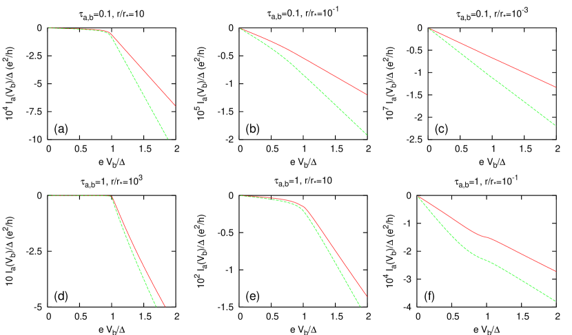
Figure 2: Variation of the normalized crossed current $I_{a}(V_{b})/\Delta$ as a function of the normalized voltage $eV_{b}/\Delta$ applied on electrode “b”, for $P=0.5$. The solid line (red) corresponds to the antiparallel alignment and the dashed line (green) to the parallel alignment. The absolute value of the crossed current is larger in the parallel alignment. Panels (a), (b) and (c) correspond to $\tau_{a,b}=0.1$, and $r/r_{*}=10^{3}$ (a), $r/r_{*}=10$ (b), and $r/r_{*}=10^{-1}$ (c). Panels (d), (e) and (f) correspond to $\tau_{a,b}=1$, and $r/r_{*}=10^{3}$ (d), $r/r_{*}=10$ (e), and $r/r_{*}=10^{-1}$ (f). We use $\eta/\Delta=10^{-3}$.

III.2 Strong energy relaxation ($\tau_{E}\ll\tau_{d}\ll\tau_{sf}$)

If we suppose strong energy relaxation ($\tau_{E}\ll\tau_{d}\ll\tau_{sf}$), the quasiparticle distribution functions in S’ are given by the Fermi distribution with quasiparticle potentials $V_{qp}^{\uparrow}$ and $V_{qp}^{\downarrow}$ for spin-up and spin-down electrons. The total current can then be calculated as an integral over energy of the transmission coefficient, and Kirchoff laws can be imposed on the integrated current. The spin-$\sigma$ quasiparticle potential $V_{qp}^{\sigma}$ is given by

$$V_{qp}^{\sigma}=\frac{T_{b}^{\sigma}N_{F}}{(T_{a}^{\sigma}+T_{b}^{\sigma})N_{F}+T_{S}N_{S}}V_{b},$$ (17)

and the current flowing from S’ to the ferromagnet “a” in the parallel and antiparallel alignments are given by the same expressions as in section III.1.

III.3 Strong spin flip ($\tau_{sf}\ll\tau_{E},\tau_{d}$)

Increasing the distance between the ferromagnetic electrodes tends to increase the transport dwell time, that can become larger than the spin flip length. The magnetoresistive effect in the crossed current decays exponentially as a function of the distance between the contacts, on a length scale set by the spin-flip length. The spin-flip length is reduced by superconducting correlations Belzig , so that the crossed current in the superconducting state is reduced, as compared to the normal case. This effect is compatible with experiments Beckmann .

In the case of strong spin-flip with energy conservation ($\tau_{sf}\ll\tau_{d}\ll\tau_{E}$), and without energy conservation ($\tau_{sf}\ll\tau_{E}\ll\tau_{d}$), the crossed current takes the form

$$I_{S^{\prime}\rightarrow a}=-2\frac{e^{2}}{h}N_{F}^{2}\frac{T_{a}T_{b}}{(T_{a}+T_{b})N_{F}+T_{S}N_{S}},$$ (18)

with $T_{a}=(T_{a}^{\uparrow}+T_{a}^{\downarrow})/2$ and $T_{b}=(T_{b}^{\uparrow}+T_{b}^{\downarrow})/2$. The crossed current due to out-of-equilibrium populations is negative, but remains finite, even though there is no magnetoresistive effect. The crossed current due to the spatially separated process tends to zero in the limit where the distance between the contacts is large compared to the superconducting coherence length. This may be used in experiments to determine whether the large distance behavior is due to out-of-equilibrium spin populations, or to the spatially separated processes.

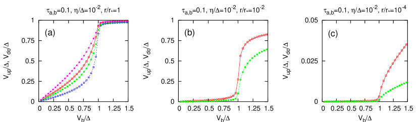
Figure 3: (a) Variation of the normalized quasiparticle potentials $V_{qp}^{\uparrow}(V_{b})/\Delta$ and $V_{qp}^{\downarrow}(V_{b})/\Delta$ as a function of $V_{b}/\Delta$, for $\eta/\Delta=10^{-2}$, $\tau_{a,b}=0.1$. The three panels correspond to $r/r_{*}=1$ (a), $r/r_{*}=10^{-2}$ (b), and $r/r_{*}=10^{-4}$ (c). The different curves correspond to $V_{qp}^{\uparrow}(V_{b})$ in the parallel (P) alignment (red, $\Box$), and to $V_{qp}^{\downarrow}(V_{b})$ in the P alignment (green, $\blacksquare$). $V_{qp}^{\uparrow}(V_{b})$ is larger than $V_{qp}^{\downarrow}(V_{b})$. On panel (a) we have shown to $V_{qp}^{\uparrow}(V_{b})$ in the antiparallel (AP) alignment (blue, $\circ$), and to $V_{qp}^{\downarrow}(V_{b})$ in the antiparallel (AP) alignment (violet, $\bullet$). We shown on the P case on panels (b) and (c) since $V_{qp}^{\uparrow,P}(V_{b})/\Delta\simeq V_{qp}^{\downarrow,AP}(V_{b})/\Delta$ and $V_{qp}^{\uparrow,AP}(V_{b})/\Delta\simeq V_{qp}^{\downarrow,P}(V_{b})/\Delta$ in these cases.

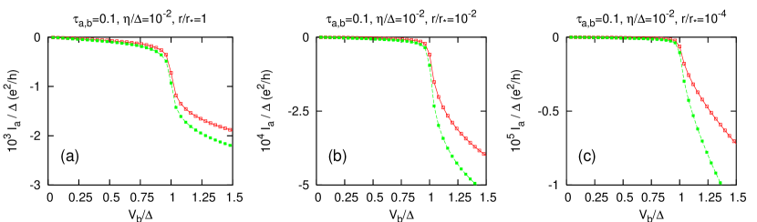
Figure 4: (a) Variation of the crossed current $I_{a}(V_{b})$ as a function of $V_{b}/\Delta$, for $\eta/\Delta=10^{-2}$, $\tau_{a,b}=0.1$. The three panels correspond to $r=1$ (a), $r=10^{-2}$ (b), and $r=10^{-4}$ (c). The different curves correspond to $I_{a}(V_{b})$ in the antiparallel alignment (red, $\Box$), and to $I_{a}(V_{b})$ in the parallel alignment (green, $\blacksquare$). The absolute value of the crossed current is larger in the parallel alignment.

IV Numerical results

IV.1 FSF double junction with weak energy relaxation

In the case of weak energy relaxation ($\tau_{d}\ll\tau_{E}\ll\tau_{sf}$) we describe S’ by a distribution function $f_{S^{\prime}}(\omega)$, supposed to be uniform in space within S’, and determined in such a way as to impose current conservation for each energy, similarly to section III.1. Within the numerical approach we can treat the full voltage dependence of the transmission coefficients, for arbitrary interface transparencies. The quasiparticle transmission coefficients deduced from Ref. Cuevas, are given in Appendix A.

The variations of the sequential tunneling crossed current $I_{a}(V_{b})$ in the parallel and antiparallel alignments are shown on Fig. 2 for $\tau_{a,b}=0.1$ and $\tau_{a,b}=1$. The absolute value of the crossed current is larger in the parallel alignment than in the antiparallel alignment (which coincides with the normal state behavior). For small values of $r/r_{*}$ the crossed conductance for $eV_{b}>\Delta$ is almost equal to the crossed conductance for $eV_{b}<\Delta$, in agreement with the argument given in section III.1.

IV.2 FSF double junction with strong energy relaxation

The case of strong energy relaxation ($\tau_{E}\ll\tau_{d}\ll\tau_{sf}$) can be obtained with low transparency interfaces in the trilayer geometry since the transport dwell time can be sufficiently long in this case. This case is likely to be irrelevant to the experiments by Beckmann et al.Beckmann involving highly transparent FS interfaces, but is of interest for future experiments with tunnel interfaces in the trilayer geometry. The quasiparticle potentials $V_{qp}^{\uparrow}$ and $V_{qp}^{\downarrow}$ are calculated self-consistently in such a way that the integrated current satisfies Kirchoff law separately in the spin-up and spin-down channels. For the sake of generality we do not treat only the case $r/r_{*}\gtrsim 1$, relevant to the trilayer geometry, but use also $r/r_{*}\ll 1$.

The variation of the normalized self-consistent quasiparticle potentials $eV_{qp}^{\uparrow}/\Delta$ and $eV_{qp}^{\downarrow}/\Delta$ as a function of $V/\Delta$ are shown on Fig. 3 for different values of $r$ and for small interface transparencies ($\tau_{a,b}=0.1$). For $r/r_{*}=1$, the normalized quasiparticle potentials $eV_{qp}^{\uparrow}/\Delta$ and $eV_{qp}^{\downarrow}/\Delta$ increase from $0$ to a value close to unity as $eV_{b}$ increases from $0$ to $\Delta$. The quasiparticle potentials are much reduced as $r/r_{*}$ decreases, due to the fact that the superconductor S tends to reduce the quasiparticle potentials in S’ as the number of channels of the SS’ contact increases. The quasiparticle potentials for $r/r_{*}=10^{-2}$ and $r/r_{*}=10^{-4}$ are mostly determined by the current flowing from S to S’ and from S’ to the ferromagnet “b”. We thus obtain $V_{qp}^{\uparrow,P}(V_{b})/\Delta\simeq V_{qp}^{\downarrow,AP}(V_{b})/\Delta$ and $V_{qp}^{\uparrow,AP}(V_{b})/\Delta\simeq V_{qp}^{\downarrow,P}(V_{b})/\Delta$, where P and AP correspond to the parallel and antiparallel alignments. These relations are due to the fact that the orientation of the ferromagnet “b” is reversed when going from the parallel (P) to the antiparallel (AP) spin orientation.

The variation of the crossed current $I_{a}(V_{b})$ as a function of $V_{b}$ is shown on Fig. 4 for the same parameters as on Fig. 3. The subgap crossed current becomes very small for small values of $r/r_{*}$, due to the fact that the self-consistent quasiparticle potentials are also very small. The absolute value of the crossed current is larger in the parallel alignment than in the parallel alignment.

V Conclusion

To conclude we have discussed a model of sequential tunneling crossed conductance based on out-of-equilibrium spin populations in the superconductor. The case of strong energy relaxation is expected to be realized for small interface transparencies in the trilayer geometryTakahashi ; Zheng ; Bozovic ; Yamashita ; Brataas , where the transport dwell time can be larger than the energy relaxation time. In the other case of highly transparent interfaces corresponding to the experiment by Beckmann et al.Beckmann , the transport dwell time is expected to be much smaller so that elastic transport can apply. The geometrical effects are encoded in a parameter $r$, very small in the geometry with lateral contacts of the experiment by Beckmann et al.Beckmann . Another small parameter is $\eta/\Delta$, proportional to the residual density of states within the superconducting gap. There exists a cross-over value $r_{*}$ such that for $r\ll r_{*}$ the crossed conductance is almost voltage-independent in the elastic model. The values of $\eta/\Delta$ used in the literatureCuevas ; Pekola indicate that the condition $r\ll r_{*}$ is verified in the experiment by Beckmann et al.Beckmann . It is found experimentally that for the smallest distance between the ferromagnets the crossed conductance is the same in the superconducting and normal phases, which can be successfully reproduced by the model of sequential tunneling. Therefore a very small residual density of state within the superconducting gap can lead to a sequential tunneling current in the geometry with lateral contacts, compatible with experiments, which is our main conclusion. In the regime of strong energy relaxation, not relevant to the experiments by Beckmann et al.Beckmann , the crossed conductance above the superconducting gap is much larger than the crossed conductance below the superconducting gap. Contrary to the elastic case, there exists a peak in the crossed conductance for $eV_{b}\simeq\Delta$ (corresponding to a large slope in the crossed current $I_{a}(V_{b})$ on Fig. 4).

In the case of tunnel interfaces, the crossed conductance due to the spatially separated processes is positive in the antiparallel alignmentFalci ; MF-PRB while the sequential tunneling crossed conductance is negative. Tunnel interfaces would thus constitute an experimental test of the possible effects. Replacing the ferromagnets by normal metalsRusso with tunnel interfaces in the geometry used by Beckmann et al.Beckmann would also be of interest. On the theoretical side it would be useful to investigate the spatial dependence of the out-of-equilibrium phenomena, and investigate a more microscopic model in which the size of the out-of-equilibrium region would be controlled by the inverse proximity effect. It would be also interesting to use quasi-classical theory for describing a diffusive superconductorBelzig .

Appendix A Transmission coefficients of a FS interface

The different terms contributing to subgap and quasiparticle transport at a FS interface are derived in Ref. Cuevas, by Keldysh Green’s function methods. In this Appendix we just recall these results and assume non equilibrium distribution functions in the superconductor.

A first term in the spin-up quasiparticle current corresponds to transmission without branch crossing:

$$I_{\rm qp,e\uparrow}^{(1)}=\int T_{e,\uparrow,{\rm loc}}^{(1)}(\omega)\left[f_{S^{\prime}}^{(\uparrow)}(\omega)-n_{F}(\omega-eV_{a})(\omega)\right]d\omega,$$ (19)

with

$$T_{e,\uparrow,{\rm loc}}^{(1)}(\omega)=4\pi^{2}t_{a}^{2}\frac{e}{h}\rho_{a,a}^{1,1}\rho_{\alpha,\alpha}^{1,1}(\omega)\left|1+t_{a}G_{a,\alpha}^{1,1,A}(\omega)\right|^{2}.$$ (20)

A second term in the quasiparticle current corresponds to transmission with branch crossingBTK :

$$I_{\rm qp,e\uparrow}^{(2)}=\int T_{e,\uparrow,{\rm loc}}^{(2)}(\omega)\left[f_{S^{\prime}}^{(\uparrow)}(\omega)-n_{F}(\omega+eV_{a})\right]d\omega,$$ (21)

with

$$T_{e,\uparrow,{\rm loc}}^{(2)}(\omega)=4\pi^{2}t_{a}^{2}\frac{e}{h}\rho_{a,a}^{2,2}\rho_{\alpha,\alpha}^{1,1}(\omega)\left|t_{a}G_{a,\alpha}^{1,2,A}(\omega)\right|^{2}.$$ (22)

A spin-up electron from the ferromagnet “a” is transmitted in the superconductor while a Cooper pair is annihilated in the superconductor therefore producing a net transfer of a spin-down hole in the superconductor.

The third term in the quasiparticle current is given by

$$I_{\rm qp,e\uparrow}^{(3)}=\int T_{e,\uparrow,{\rm loc}}^{(3)}(\omega)\left[n_{F}(\omega-eV_{a})-n_{F}(\omega+eV_{a})\right]d\omega,$$ (23)

with

$$T_{e,\uparrow,{\rm loc}}^{(3)}(\omega) = -4\pi^{2}t_{a}^{3}\frac{e}{h}\rho_{a,a}^{1,1}\rho_{\alpha,\alpha}^{1,2}(\omega)$$

$$\times \mbox{Re}\left\{\left[1+t_{a}G_{\alpha,a}^{1,1,R}(\omega)\right]G_{a,\alpha}^{2,1,A}(\omega)\right\}.$$

The density of state prefactors in the first term of Eq. (23) are given by $\rho_{a,\uparrow}\rho_{a,\downarrow}\rho_{\alpha,\alpha}^{1,2}$ if we use $G_{a,\alpha}^{2,1,A}=-i\pi t_{a}\rho_{a,a}^{2,2}G_{\alpha,\alpha}^{2,1,A}$. This process therefore corresponds to the transmission of a spin-up electron from the ferromagnet to the superconductor. At the same time a particle-hole excitation is created at the interface, the spin-down hole is backscattered in the ferromagnet and the spin-up electron is transmitted is the superconductor. This process in the quasiparticle channel is reminiscent of the Andreev reflection term.

References

- (1) C.J. Lambert and R. Raimondi, J. Phys.: Condens. Matter 10, 901 (1998).
- (2) F.J. Jedema, B.J. van Wees, B.H. Hoving, A.T. Filip and T.M. Klapwijk, Phys. Rev; B 60, 16549 (1999).
- (3) M. Tinkham, Introduction to superconductivity, Second Edition, McGraw-Hill (1996).
- (4) S. Takahashi, H. Imamura, and S. Maekawa Phys. Rev. Lett. 82, 3911 (1999).
- (5) Z. Zheng, D.Y. Xing, G. Sun, and J. Dong, Phys. Rev. B 62, 14326 (2000).
- (6) M. Bozovic and Z. Radovic, Phys. Rev. B 66, 134524 (2002).
- (7) T. Yamashita et al., Phys. Rev. B 67, 094515 (2003).
- (8) J. Johansson, V. Korenivski, D. B. Haviland, and A. Brataas Phys. Rev. Lett. 93, 216805 (2004).
- (9) C.J. Lambert, J. Koltai, and J. Cserti, in Towards the controllable quantum states (Mesoscopic superconductivity and spintronics, p. 119, Eds H. Takayanagi and J. Nitta, World Scientific (2003).
- (10) G. Deutscher and D. Feinberg, App. Phys. Lett. 76, 487 (2000).
- (11) G. Falci, D. Feinberg, and F.W.J. Hekking, Europhysics Letters 54, 255 (2001).
- (12) R. Mélin, J. Phys.: Condens. Matter 13, 6445 (2001);
- (13) R. Mélin and S. Peysson, Rev. B 68, 174515 (2003).
- (14) N.M. Chtchelkatchev, I.S. Burmistrov, Phys. Rev. B 68, 140501 (2003).
- (15) R. Mélin, H. Jirari and S. Peysson, J. Phys.: Condens. Matter 15, 5591 (2003).
- (16) D. Feinberg, Eur. Phys. J. B 36, 419 (2003).
- (17) D. Sanchez, R. Lopez, P. Samuelson and M. Buttiker, Phys. Rev. B 68, 214501 (2003).
- (18) G. Bignon, M. Houzet, F. Pistolesi, and F. W. J. Hekking, cond-mat/0310349.
- (19) R. Mélin and D. Feinberg, Phys. Rev. B 70, 174509 (2004).
- (20) D. Beckmann, H.B. Weber and H.v. Löhneysen, Phys. Rev. Lett. 93, 197003 (2004).
- (21) S. Russo, M. Kroug, T.M. Klapwijk, and A.F. Morpurgo, cond-mat/0501564.
- (22) J. Clarke, Phys. Rev. Lett. 28, 1363 (1972); M. Tinkham and J. Clarke, ibid 28, 1366 (1972).
- (23) C. Caroli, R. Combescot, P. Nozières and D. Saint-James, J. Phys. C: Solid St. Phys. 4, 916 (1971); ibid. 5, 21 (1972).
- (24) J.C. Cuevas, A. Martín-Rodero and A. Levy Yeyati, Phys. Rev. B 54, 7366 (1996).
- (25) S.B. Kaplan et al., Phys. Rev. B 14, 4854 (1976).
- (26) J.P. Pekola et al., Phys. Rev. Lett. 92, 056804 (2004).
- (27) G.E. Blonder, M. Tinkham, and T.M. Klapwijk, Phys. Rev. B 25, 4515 (1982).
- (28) J.P. Morten, A. Brataas, and W. Belzig, Phys. Rev. B 70, 212508 (2004); J.P. Morten, A. Brataas, and W. Belzig, cond-mat/0501566.