Exploring Hydrodynamic Closures for the Lid-driven Micro-cavity

Abstract

A minimal kinetic model is used to study analytically and numerically flows at a micrometer scale. Using the lid-driven microcavity as an illustrative example, the interplay between kinetics and hydrodynamics is quantitatively visualized. The validity of various theories of non-equilibrium thermodynamics of flowing systems is tested in this nontrivial microflow.

1 Introduction

Flows in microdevices constitute an emerging application field of fluid dynamics Beskok & Karniadakis (2001). Despite impressive experimental progress, theoretical understanding of microflows remains incomplete. For example, even though microflows are highly subsonic, the assumption of incompressible fluid motion is often questionable (see, e. g. Zheng et al. (2002)). Interactions between the relaxation of density variations, the rarefaction and the flow geometry are not completely understood. One of the reasons for this is the lack of commonly accepted models for efficient simulations of microflows.

In principle, microflows can be studied using molecular level methods, such as the Direct Simulation Monte Carlo (DSMC) method Bird (1994). However, molecular dynamics methods face severe limitations for subsonic flows. The number of particles required for simulations in realistic geometries with large aspect ratios and the number of time steps needed to reach the statistical steady state are prohibitively high Oran et al. (1998) (the time step of DSMC is $\sim 10^{-10}$sec, while relevant physical time-scales are $\sim 10-100$sec). Moreover, a detailed microscopic description in terms of the particle distribution function is not necessary for design/endineering purposes. Thus, development of reduced models enabling efficient simulations is an important issue.

In this paper we consider a two-dimensional minimal kinetic model with nine discrete velocities Karlin et al. (1999); Ansumali et al. (2003). It has been recently shown by several groups Ansumali & Karlin (2002b); Ansumali et al. (2004); Niu et al. (2003); Succi & Sbragaglia (2004) that this model compares well with analytical results of kinetic theory Cercignani (1975) in simple flow geometries (channel flows), as well as with molecular dynamics simulations. The focus of this paper is the validation of several theoretical models of (extended) hydrodynamics versus direct numerical simulation in a non-trivial flow. For that purpose, we considered the flow in a lid-driven cavity. We will visualize the onset of the hydrodynamic description, the effect of the boundaries etc.

The paper is organized as follows: For completeness, the kinetic model Karlin et al. (1999); Ansumali et al. (2003) is briefly presented in section 2. In section 3, we show the relation of our model to the well-known Grad moment system derived from the Boltzmann kinetic equation Grad (1949). We compare analytically the dispersion relation for the present model and the Grad moment system. This comparison reveals that the kinetic model of section 2 is a superset of Grad’s moment system. In section 4, a parametric numerical study of the flow in a micro-cavity is presented. Results are also compared to a DSMC simulation. In section 5, the reduced description of the model kinetic equation is investigated, and a visual representation quantifying the onset and breakdown of the hydrodynamics is discussed. We conclude in section 6 with a spectral analysis of the steady state flow and some suggestions for further research Theodoropoulos et al. (2000, 2004); Kevrekidis et al. (2003, 2004).

2 Minimal kinetic model

We consider the discrete velocity model with the following set of nine discrete velocities:

$$\begin{split}c_{x}&=\left[0,1,0,-1,0,1-1,-1,1\right],\quad c_{y}=\left[0,0,1,0,-1,1,1,-1,-1\right].\end{split}$$ (1)

The local hydrodynamic fields are defined in terms of the discrete population, $f_{i}$, as:

$$\sum_{i=1}^{9}f_{i}\{1,\,c_{x\,i},\,c_{y\,i}\}=\{\rho,\,j_{x},\,j_{y}\},$$ (2)

where $\rho$ is the local mass density, and $j_{\alpha}$ is the local momentum density of the model. The populations $f_{i}\equiv f(\mathbf{x},\mathbf{c}_{i},t)$ are functions of the discrete velocity $\mathbf{c}_{i}$, position $\mathbf{x}$ and time $t$. We consider the following kinetic equation for the populations (the Bhatnagar-Gross-Krook single relaxation time model):

$$\partial_{t}f_{i}+\mathbf{c}_{i}\cdot\partial_{\mathbf{x}}f_{i}=-\frac{1}{\tau}\left(f_{i}-f_{i}^{\rm eq}(f)\right),$$ (3)

where $\tau$ is the relaxation time, and $f_{i}^{\rm eq}$ is the local equilibrium Ansumali et al. (2003):

$$\begin{split}f^{\rm eq}_{i}=\rho W_{i}\left(2-\sqrt{1+3{u_{x}}^{2}}\right)\left(2-\sqrt{1+3{u_{y}}^{2}}\right)\left(\frac{2u_{x}+\sqrt{1+3{u_{x}}^{2}}}{1-u_{x}}\right)^{c_{xi}}\left(\frac{2u_{y}+\sqrt{1+3{u_{y}}^{2}}}{1-u_{y}}\right)^{c_{yi}},\end{split}$$ (4)

where $u_{\alpha}=j_{\alpha}/\rho$, and the speed of sound is $c_{\rm s}=1/\sqrt{3}$. The local equilibrium distribution $f_{i}^{\rm eq}$ is the minimizer of the discrete $H$ function Karlin et al. (1999); Ansumali et al. (2003):

$$H=\sum_{i=1}^{9}f_{i}\ln\left(\frac{f_{i}}{W_{i}}\right),\;\mbox{with weights}\quad W=\left[\frac{16}{36},\frac{4}{36},\frac{4}{36},\frac{4}{36},\frac{4}{36},\frac{1}{36},\frac{1}{36},\frac{1}{36},\frac{1}{36}\right],$$ (5)

under the constraints of the local hydrodynamic fields (2). Note the important factorization over spatial components of the equilibrium (4). This is similar to the familiar property of the local Maxwell distribution, and it distinguishes (4) among other discrete-velocity equilibria.

In the hydrodynamic regime, the model recovers the Navier-Stokes equation with viscosity coefficient $\mu=p\tau$, where $p=\rho c_{\rm s}^{2}$ is the pressure (see section 5). The diffusive-wall approximation Ansumali & Karlin (2002b) is used for wall boundary conditions.

3 Grad’s moment system and the minimal kinetic model

3.1 The moment system

It is useful to represent the discrete velocity model (3) in the form of a moment system. For simplicity, we shall consider the linearized version of the model. Note that linearization is required only for the collision term on the right hand side of equation (3). This is at variance with Grad’s moment systems Grad (1949) where the advection terms are nonlinear as well. We choose the following nine non-dimensional moments as independent variables:

$${M}=\left[\frac{\rho}{\rho_{0}},\frac{j_{x}}{\rho_{0}c_{\rm s}},\frac{j_{y}}{\rho_{0}c_{\rm s}},\frac{P}{\rho_{0}c_{\rm s}^{2}},\frac{N}{\rho_{0}c_{\rm s}^{2}},\frac{P_{xy}}{\rho_{0}c_{\rm s}^{2}},\frac{q_{x}}{2\rho_{0}c_{\rm s}^{3}},\frac{q_{y}}{2\rho_{0}c_{\rm s}^{3}},\frac{\psi}{2\rho_{0}c_{\rm s}^{4}}\right],$$ (6)

where

$$\psi=R_{yyyy}+R_{xxxx}-2R_{xxyy},$$ (7)

is a scalar obtained from 4^th-order moments $R_{\alpha\beta\gamma\theta}=\sum_{i=1}^{9}f_{i}c_{\alpha i}c_{\beta i}c_{\gamma i}c_{\theta i}$, ${N}=\sum_{i=1}^{9}f_{i}(c_{xi}^{2}-c_{yi}^{2})/2\equiv{(P_{xx}-P_{yy})}/{2}$ is the difference of the normal stresses, $P=\sum_{i=1}^{9}f_{i}c_{i}^{2}$ is the trace of the pressure tensor, and $q_{\alpha}=\sum_{i=1}^{9}f_{i}c_{\alpha i}c_{i}^{2}$ is the energy flux obtained by contraction of the third-order moment $Q_{\alpha\beta\gamma}=\sum_{i=1}^{9}f_{i}c_{\alpha i}c_{\beta i}c_{\gamma i}$. Time and space are made non-dimensional in such a way that for a fixed system size $L$ they are measured in the units of mean free time and mean free path, respectively: $\mathbf{x}^{\prime}=\mathbf{x}/(L{\rm Kn}),t^{\prime}=t/\tau$, where ${\rm Kn}=\tau c_{\rm s}/L$ is the Knudsen number. The linearized equations for the moments $M$ (6) read (from now on we use the same notation for the non-dimensional variables):

$$\begin{split}\partial_{t}\rho+\,\partial_{x}j_{x}+\partial_{y}j_{y}&=0,\\ \partial_{t}j_{x}+\partial_{x}\left(P+N\right)+\partial_{y}P_{xy}&=0,\\ \partial_{t}j_{y}+\partial_{x}P_{xy}+\partial_{y}\left(P-N\right)&=0,\\ \partial_{t}P+\partial_{x}q_{x}+\partial_{y}q_{y}&=\left({\rho}-P\right),\\ \partial_{t}N+\partial_{x}\left(q_{x}-Q_{xyy}\right)-\partial_{y}\left(q_{y}-Q_{yxx}\right)&=-N,\\ \partial_{t}P_{xy}+\partial_{x}Q_{yxx}+\partial_{y}Q_{yyx}&=-P_{xy},\\ \partial_{t}q_{x}+\partial_{x}R_{xx\alpha\alpha}+\partial_{y}R_{xy\alpha\alpha}&=\left(2j_{x}-q_{x}\right),\\ \partial_{t}q_{y}+\partial_{x}R_{xy\alpha\alpha}+\partial_{y}R_{yy\alpha\alpha}&=\left(2j_{y}-q_{y}\right),\\ \partial_{t}\psi+\partial_{x}\left(j_{x}-q_{x}\right)+\partial_{y}\left(j_{y}-q_{y}\right)&=\left(2\rho-\psi\right).\end{split}$$ (8)

Furthermore, by construction of the discrete velocities (1), the following relations are satisfied:

$$Q_{xyy}=2q_{x}-{3}j_{x},\quad Q_{yxx}=2q_{y}-{3}j_{y},$$ (9)

$$R_{xy\alpha\alpha}=3P_{xy},\;\;R_{xx\alpha\alpha}=3\left(P+\frac{1}{2}N\right)-\frac{1}{2}\psi,\;\;R_{yy\alpha\alpha}=3\left(P-\frac{1}{2}N\right)-\frac{1}{2}\psi.$$ (10)

Apart from the lack of conservation of the energy and linearity of the advection, equation (8) is quite similar to Grad’s two-dimensional $8$-moment system . However, in the present case a particular component of the 4^th-order moment is also included as a variable. In other words, Grad’s non-linear closure for the 4^th-order moment is replaced by an evolution equation with a linear advection term. We note here that while the formulation of boundary conditions for Grad’s moment system remains an open problem, the boundary conditions for the extended moment system (system 8, 9, and 10) are well established through its discrete-velocity representation (3) Ansumali & Karlin (2002b). We also note that like any other Grad’s system the present model reproduces the Navier-Stokes equation in the hydrodynamic limit Karlin et al. (1999); Ansumali et al. (2003). The moment system (8) reveals the meaning of the densities appearing in model: The dimensionless density is the dimensionless pressure of the real fluid in the low Mach number limit, while the momentum flux density should be identified with the velocity in the incompressible limit. With this identification, we shall compare the moment system (8) with Grad’s system.

3.2 One-dimensional Grad’s moment system

Since energy is not conserved by the model (3), the comparison will be with another Grad moment system which (for $D=3$) is usually referred to as the $10$-moment system . For one-dimensional flows, the linearized Grad’s $10$-moment system can be written as Gorban & Karlin (2005); Karlin & Gorban (2002):

$$\begin{split}\partial_{t}p+\gamma\partial_{x}u_{x}=0,\quad\partial_{t}u_{x}+\partial_{x}P_{xx}=0,\quad\partial_{t}P_{xx}+3\partial_{x}u_{x}=-\left(P_{xx}-p\right),\end{split}$$ (11)

where $\gamma$ is the ratio of the specific heats of the fluid, and $\gamma=(D+2)/D$ for a $D$-dimensional dilute gas. This model can be described in terms of its dispersion relation, which upon substitution of the solution in the form $\sim\exp{\left(\omega t+ikx\right)}$ reads:

$$\omega^{3}+\omega^{2}+3k^{2}\omega+\gamma k^{2}=0.$$ (12)

The low wave-number asymptotic represents the large-scale dynamics (hydrodynamic scale of ${\rm Kn}\ll 1$), while the high-wave number limit represent the molecular scales quantified by ${\rm Kn}\gg 1$. The low wave number (${\rm Kn}\ll 1$) asymptotic, $\omega_{\rm l}$, and the large wave number (${\rm Kn}\gg 1$) asymptotic, $\omega_{\rm h}$, are:

$$\omega_{\rm l}=\left\{\frac{(-3+\gamma)}{2}k^{2}\pm i\sqrt{\gamma}k,\;-1-(-3+\gamma)k^{2}\right\},\;\;\omega_{\rm h}=\left\{\frac{(-3+\gamma)}{6}\pm i\sqrt{3}k,\;-\frac{\gamma}{3}\right\}.$$ (13)

The two complex conjugate modes (acoustic modes) of the $O(k^{2})$ dynamics, are given by the first two roots of $\omega_{\rm l}$, and represent the hydrodynamic limit (the Navier-Stokes approximation) of the model. The third root in this limit is real and negative, corresponding to the relaxational behavior of the non-hydrodynamic variable (stress): the dominant contribution (equal to $-1$) is the relaxation rate towards the equilibrium value, while the next-order correction suggests slaving of viscous forces, which amounts to the constitutive relation for stress ($(-3+\gamma)/2k^{2}$ ). Furthermore, the $k^{2}$ dependence of the relaxation term justifies the assumption of scale separation (the higher the wave-number, the faster the relaxation). The real part of the high wave-number solution $\omega_{\rm h}$ is independent of $k$, which shows that the relaxation at very high Knudsen number is the same for all wavenumbers (so-called “Rosenau saturation” Gorban & Karlin (1996); Slemrod (1998)). Thus, the assumption of scale-separation is not valid for high Knudsen number dynamics.

3.3 Dispersion relation for the moment system

The dispersion relation for the one-dimensional version of the moment system (8) (i.e. neglecting all derivatives in the $y$-direction) reads:

$$(\omega^{3}+\omega^{2}+3k^{2}\omega+k^{2})(\omega^{3}+2\omega^{2}+(3k^{2}+1)\omega+k^{2})(1+\omega)((1+\omega^{2})+2k^{2})=0.$$ (14)

The real parts of the roots of this equation (attenuation rates ${\rm Re}[\omega(k)]$) are plotted in Fig. 1 as functions of the wave vector $k$.

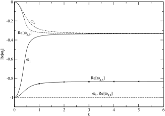
Figure 1: Real part of the solutions of the dispersion relation (equation (14)). Roots $\omega_{2,3}$ and $\omega_{1}$ correspond to Grad’s subsystem (equation (11)). The real-valued root $\omega_{6}$ and the complex conjugate roots $\omega_{2,3}$ are extended hydrodynamic modes.

It is clear that for one-dimensional flows, the dynamics of three of the moments ($\rho$, $j_{x}$, and $P$) are decoupled from the rest of the variables, and follows of the dynamics of the one-dimensional Grad’s moment system (11) with $\gamma=1$.

The similarity between Grad’s moment system and the present model is an important fingerprint of the kinetic nature of the latter . Note that in the case of two-dimensional flows, the agreement between the present model and Grad’s system is only qualitative. The present moment system is isotropic only up to $O(k^{2})$. Thus, the dispersion relation of the model (3) is expected to match the one of Grad’s system only up to the same order. In the hydrodynamic and slip-flow regime addressed below, this order of isotropy is sufficient. In the presence of boundaries and/or non-linearities, it is necessary to resort to numerics. Below we use the entropic lattice Boltzmann discretization method (ELBM) of the model (3).

4 Flow in a lid-driven micro-cavity

The two-dimensional flow in a lid-driven cavity was simulated with ELBM over a range of Knudsen numbers defined as ${\rm Kn}={\rm Ma}/\rm Re$. In the simulations, the Mach number was fixed at ${\rm Ma}=0.01$ and the Reynolds number, $\rm Re$, was varied. Initially, the fluid in the cavity is at rest and the upper wall of the domain is impulsively set to motion with $u_{\rm lid}=c_{\rm s}{\rm Ma}$. Diffusive boundary conditions are imposed at the walls Ansumali & Karlin (2002b), and the domain was discretized using $151$ points in each spatial direction. Time integration is continued till the steady state is reached; matrix-free, Newton-Krylov fixed point algorithms for the accelerated computation of the steady state are also being explored Theodoropoulos et al. (2000).

4.1 Validation with DSMC simulation of the micro-cavity

In the hydrodynamic regime, the model was validated using results available from continuum simulations Ansumali & Karlin (2002a). For higher ${\rm Kn}\sim 0.1$, we compared our results with the DSMC simulation of Jiang et al. (2003). Good agreement between the DSMC simulation and the ELBM results can be seen in Fig. 2. It can be concluded, that even for finite Knudsen number, the present model provides semi-quantitative agreement, as far as the flow profile is concerned. We remind here again, that the dimensionless density in the present model corresponds to the dimensionless pressure of a real fluid so that, for quantitative comparison, the density of ELBM model should be compared with the pressure computed from DSMC.

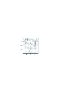
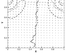
Figure 2: Flow in a micro-cavity for ${\rm Kn}=0.1$ and ${\rm Ma}=0.14$: DSMC simulation Jiang et al. (2003) (left) , velocity vector plot and density isolines from ELBM (solid lines) with the DSMC density isolines (dashed lines) superimposed (right).

4.2 Parametric study of the flow in the micro-cavity

Fig. 3 shows the dimensionless density profiles with the streamlines superimposed for ${\rm Kn}=0.001,0.01,0.1$. For ${\rm Kn}=0.001$ (${\rm Re}=10$), the behavior expected from continuum simulations with a large central vortex and two smaller recirculation zones close to the lower corners can be observed. As the Knudsen number is increased, the lower corner vortices shrink and eventually disappear and the streamlines tend to align themselves with the walls.

The density profiles, as a function of ${\rm Kn}$, demonstrate that the assumption of incompressibility is well justified only in the continuum regime, where the density is essentially constant away from the corners. This observation is consistent with the conjecture that incompressibility requires smallness of the Mach as well as of the Knudsen number. In hydrodynamic theory, the density waves decay exponentially fast (with the rate of relaxation proportional to $\rm{\rm Kn}$) leading effectively to incompressibility. Thus, it is expected that the onset of incompressibility will be delayed as the Knudsen number increases.

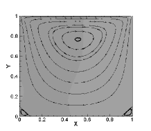
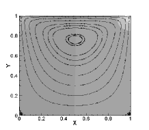
Figure 3: Density isocontours for (a) ${\rm Kn}=0.001$, (b)${\rm Kn}=0.01$ , and (c) ${\rm Kn}=0.1$ (the variation of the density is $0.995\leq\rho\leq 1.005$). Superimposed are the streamlines.

5 Reduced description of the flow

The data from the direct simulation of the present kinetic model were used to validate the effectiveness of different closure approximations of kinetic theory in the presence of kinetic boundary layers in a fairly non-trivial flow, and to gain some insight about the required modification of the closure approximations in the presence of boundary layers. In this section, we will present such an analysis for two widely used closure methods, the Navier-Stokes approximation of the Chapman-Enskog expansion and Grad’s moment closure.

5.1 The Navier-Stokes approximation

The Chapman-Enskog analysis Chapman & Cowling (1970) of the model kinetic equation leads to a closure relation for the non-equilibrium part of the pressure tensor as (the Navier-Stokes approximation):

$$\sigma_{xy}=-{\tau}c_{\rm s}^{2}(\partial_{y}j_{x}+\partial_{x}j_{y}).$$ (15)

Fig. 4 shows a scatter plot of the $xy$ component of the non-equilibrium part of the pressure tensor $P_{xy}-P_{xy}^{\rm eq}$, versus that computed from the Navier-Stokes approximation of the Chapman-Enskog expansion (15). The upper row is the scatter plot for all points in the computational domain, while the lower row is the scatter plot obtained after removal of the boundary layers close to the four walls of the cavity, corresponding to approximately $10$ mean-free paths. In all plots, the dashed straight line of slope equal to one corresponds to Navier-Stokes behavior. These plots clearly reveal that the Navier-Stokes description is valid away from the walls in the continuum as well as in the slip flow regime. On the other hand, it fails to represent hydrodynamics in the kinetic boundary layer.

Perhaps the most interesting observation from Fig. 4 is the coherent, curve-like structure of the off-Navier-Stokes points. These trajectories tend to the Navier-Stokes approximation as to an attractive sub-manifold. This structure resembles the trajectories of solutions to the invariance equation Gorban & Karlin (2005); Gorban et al. (2004) observed, in particular, in a similar problem of derivation of hydrodynamics from Grad’s systems (see, e. g. Karlin & Gorban (2002), p. 831, Fig. 12). A link between solutions to invariance equations and the present simulations is an intriguing subject for further study. In the next subsection, we shall explore Grad’s closure approximation for the present flow.

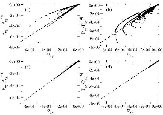
Figure 4: Scatter plot of the non-equilibrium part of the off-diagonal component of the pressure tensor $P_{xy}-P_{xy}^{\rm eq}$ and corresponding value computed from Navier-Stokes approximation $\sigma_{xy}$ (15) for all points in the domain ((a) and (b)), and after the removal of the boundary layer corresponding to approximately $10$ mean-free path ((c) and (d)). Fig. (a,c) correspond to ${\rm Kn}=0.001$, while Fig. (b,d) correspond to ${\rm Kn}=0.01$. Navier-Stokes behavior is indicated by the straight line of slope equal to one.

5.2 Grad’s approximation

In contrast to the Chapman-Enskog method, the Grad method has an advantage that the approximations are local in space, albeit with an increased number of fields. As the analysis of section 3 suggests, the dynamics of the density, momentum and pressure tensor are almost decoupled from the rest of the moments, at least away from boundaries. This motivates the Grad-like approximation for the populations,

$$\begin{split}f_{i}^{\rm Grad}=W_{i}\left[\rho+\frac{j_{\alpha}c_{i\,\alpha}}{c_{\rm s}^{2}}+\frac{1}{2\,c_{\rm s}^{4}}\,\left(P_{\alpha\beta}-\delta_{\alpha\beta}\rho c_{\rm s}^{2}\right)\left(c_{i\,\alpha}c_{i\,\beta}-c_{\rm s}^{2}\delta_{\alpha\beta}\right)\right].\end{split}$$ (16)

The set of populations parameterized by the values of the density, momentum and pressure tensor (16) is a sub-manifold in the phase space of the system (3), and can be derived in a standard way using quasi-equilibrium procedures Gorban & Karlin (2005); Gorban et al. (2004). After taking into account the time discretization, we find the closure relation for the energy flux:

$$\begin{split}q_{\alpha}^{\rm Grad}=\frac{4}{3}\left(1+\frac{p}{2\mu}\right){j_{\alpha}}-\frac{p}{2\mu}q_{\alpha}^{\rm eq}.\end{split}$$ (17)

In Fig. 5, the scatter plot of the computed energy flux $q_{x}$ and the discrete Grad’s closure $q_{x}^{\rm Grad}$ (17) is presented. Same as in Fig. 4, the off-closure points in Fig. 5 are associated with the boundary layers. The comparison of the quality with which the closure relations are fulfilled in Fig. 4 and Fig. 5 clearly indicates the advantage of that a Grad’s closure. Various strategies of a domain decomposition for a reduced simulation can be devised based on this observation. A general conclusion is that for slow flows Grad’s closure in the bulk along with the discretization of the boundary condition Ansumali & Karlin (2002b) is the optimal strategy for the simulation of microflows.

Figure 5: Scatter plot of the computed energy flux, $q_{x}$, versus Grad’s closure, $q_{x}^{\rm Grad}$: (a) ${\rm Kn}=0.001$, (b) ${\rm Kn}=0.01$.

6 Conclusions and further studies

We considered a specific example of a minimal kinetic model for studies of microflows, and compared it with other theories of nonequilibrium thermodynamics in a nontrivial flow situation. The close relationship between Grad’s moment systems and minimal kinetic models was highlighted. For the case of a driven cavity flow, different closure approximations were tested against the direct simulation data, clearly showing the failure of the closures near the boundaries. Grad’s closure for the minimal model was found to perform better than the Navier-Stokes approximation. This finding can be used to reduce the memory requirement in simulations, while preserving the advantage of locality.

In this paper, we have explored two classical closures of kinetic theory. In the future we are going to consider other closures such as the invariance correction to Grad’s closure, and especially closures based on spectral decomposition Gorban & Karlin (2005). To that end, the ELBM code was coupled with ARPACK Lehoucq et al. (1998) in order to compute the leading eigenvalues and the corresponding eigenvectors of the Jacobian field of the corresponding map at the steady state. In all cases, the eigenvalues are within the unit circle (Fig. 6(a)). The leading eigenvalue is always equal to one (reflecting mass conservation), and the corresponding eigenvector captures most of the structure of the steady state. As the Knudsen number decreases, eigenvalues tend to get clustered close to the unit circle. This happens because when the Knudsen number is small the incompressibility assumption is a good approximation, and mass is also conserved locally. The very close similarity between fig. 6(b) and fig. 4(a), reveals that states perturbed away from the steady state along the leading eigenvector are also described well by the Navier-Stokes closure.

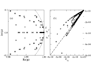
Figure 6: (a) Leading eigenvalues of the minimal kinetic model at steady state (square: Kn=$10^{-4}$, circle: Kn=$10^{-3}$, X: Kn=$10^{-2}$, +: Kn=$10^{-1}$); (b) Scatter plot as in Fig. 4(a) for a state perturbed away from the steady state along the leading eigenvector (Kn=$10^{-3}$).

Acknowledgement. Discussions with A. N. Gorban are gratefully acknowledged. The work of SA, CEF and IVK was partially supported by the Swiss Federal Department of Energy (BFE) under the project Nr. 100862 “Lattice Boltzmann simulations for chemically reactive systems in a micrometer domain”. The work of IGK was partially supported by an NSF-ITR grant and by DOE.

References

- Ansumali & Karlin (2002a) Ansumali, S. & Karlin, I. V. 2002a Entropy Function Approach to the Lattice Boltzmann Method. J. Stat. Phys. 107(1-2), 291–308.
- Ansumali & Karlin (2002b) Ansumali, S. & Karlin, I. V. 2002b Kinetic Boundary Condition for the Lattice Boltzmann Method. Phys. Rev. E 66(2), 026311.
- Ansumali et al. (2004) Ansumali, S., Karlin, I. V., Frouzakis, C. E. & Boulouchos, K. B. 2004 Entropic Lattice Boltzmann Method for Microflows. http://xxx.lanl.gov/abs/cond-mat/0412555 .
- Ansumali et al. (2003) Ansumali, S., Karlin, I. V. & Öttinger, H. C. 2003 Minimal Entropic Kinetic Models for Simulating Hydrodynamics. Europhys. Lett. 63(6), 798–804.
- Beskok & Karniadakis (2001) Beskok, A. & Karniadakis, G. E. 2001 Microflows: Fundamentals and Simulation. Springer, Berlin.
- Bird (1994) Bird, G. A. 1994 Molecular Gas Dynamics and the Direct Simulation of Gas Flows. Theory and Application of the Boltzmann Equation. Oxford University Press.
- Cercignani (1975) Cercignani, C. 1975 Theory and Application of the Boltzmann Equation. Scottish Academic Press, Edinburgh.
- Chapman & Cowling (1970) Chapman, S. & Cowling, T. G. 1970 The Mathematical Theory of Non-Uniform Gases. Cambridge University Press, Cambridge.
- Gorban & Karlin (1996) Gorban, A. N. & Karlin, I. V. 1996 Short-wave Limit of Hydrodynamics: A Soluble Example. Phys. Rev. Lett. 77, 282–285.
- Gorban & Karlin (2005) Gorban, A. N. & Karlin, I. V. 2005 Invariant Manifolds for Physical and Chemical Kinetics. Springer, Berlin Heidelberg.
- Gorban et al. (2004) Gorban, A. N., Karlin, I. V. & Zinovyev, A. Y. 2004 Constructive Methods of Invariant Manifolds for Kinetic Problems. Phys. Rep. 396, 197–403.
- Grad (1949) Grad, H. 1949 On the Kinetic Theory of Rarefied Gases. Comm. Pure Appl. Math. 2, 331–407.
- Jiang et al. (2003) Jiang, J.-Z., J., F. & Shen, C. 2003 Statistical simulation of micro-cavity flows. 23rd Int. Symposium on Rarefied Gas Dynamics pp. 784–790.
- Karlin et al. (1999) Karlin, I. V., Ferrante, A. & Öttinger, H. C. 1999 Perfect Entropy Functions of the Lattice Boltzmann Method. Europhys. Lett. 47, 182–188.
- Karlin & Gorban (2002) Karlin, I. V. & Gorban, A. N. 2002 Hydrodynamics from Grad’s Equations: What can We Learn from Exact Solutions? Ann. Phys. (Leipzig) 11, 783–833.
- Kevrekidis et al. (2003) Kevrekidis, I. G., Gear, C., Hyman, J. M., Kevrekidis, P. G., Runborg, O. & Theodoropoulos, C. 2003 Equation-free, Coarse-grained Multiscale Computation: Enabling Microscopic Simulators to Perform System -level Analysis. Comm. Math. Sci. 1, 715–762.
- Kevrekidis et al. (2004) Kevrekidis, I. G., Gear, C. W. & Hummer, G. 2004 Equation-free: the Computer-assisted Analysis of Complex, Multiscale systems. A. I. Ch. E. Journal 50 (7), 1346–1354.
- Lehoucq et al. (1998) Lehoucq, R., Sorensen, D. & Yang, C. 1998 ARPACK Users’ Guide: Solution of Large-Scale Eigenvalue Problems with Implicitly Restarted Arnoldi Methods. SIAM.
- Niu et al. (2003) Niu, X. D., Shu, C. & Chew, Y. 2003 Lattice Boltzmann BGK Model for Simulation of Micro Flows. Euro. Phys. Lett. 67, 600–606.
- Oran et al. (1998) Oran, E. S., Oh, C. K. & Cybyk, B. Z. 1998 Direct Simulation Monte Carlo: Recent Advances and Applications. Annu Rev. Fluid Mech. 30, 403–441.
- Slemrod (1998) Slemrod, M. 1998 Renormalization of the Chapman-Enskog Expansion: Isothermal Fluid Flow and Rosenau Saturation. J. Stat. Phys. 91, 285–305.
- Succi & Sbragaglia (2004) Succi, S. & Sbragaglia, M. 2004 Analytical Calculation of Slip Flow in Lattice Boltzmann Models with Kinetic Boundary Conditions. http://arxiv.org/abs/nlin.CG/0410039 .
- Theodoropoulos et al. (2000) Theodoropoulos, K., Qian, Y.-H. & Kevrekidis, I. G. 2000 “Coarse” Stability and Bifurcation Analysis Using Timesteppers: a reaction diffusion example. Proc. Natl. Acad. Sci. 97 (18), 9840–9843.
- Theodoropoulos et al. (2004) Theodoropoulos, K., Sankaranarayanan, K., Sundaresan, S. & Kevrekidis, I. G. 2004 Coarse Bifurcation Studies of Bubble Flow Lattice Boltzmann Simulations. Chem. Eng. Sci. 59, 2357–2362.
- Zheng et al. (2002) Zheng, Y., Garcia, A. L. & Alder, B. J. 2002 Comparison of Kinetic Theory and Hydrodynamics for Poiseuille Flow. J. Stat. Phys. 109, 495–505.