Can Frustration Preserve a Quasi-Two-Dimensional Spin Fluid?

Abstract

Using spin-wave theory, we show that geometric frustration fails to preserve a two-dimensional spin fluid. Even though frustration can remove the interlayer coupling in the ground-state of a classical antiferromagnet, spin layers innevitably develop a quantum-mechanical coupling via the mechanism of “order from disorder”. We show how the order from disorder coupling mechanism can be viewed as a result of magnon pair tunneling, a process closely analogous to pair tunneling in the Josephson effect. In the spin system, the Josephson coupling manifests itself as a biquadratic spin coupling between layers, and for quantum spins, these coupling terms are as large as the in-plane coupling. An alternative mechanism for decoupling spin layers occurs in classical XY models in which decoupled ”sliding phases” of spin fluid can form in certain finely tuned conditions. Unfortunately, these finely tuned situations appear equally susceptible to the strong-coupling effects of quantum tunneling, forcing us to conclude that in general, geometric frustration cannot preserve a two-dimensional spin fluid.

I Introduction

This study is motivated by recent theories of heavy electron systems tuned to an antiferromagnetic quantum critical point Rosch ; Si which propose that the formation of magnetically decoupled layers of spins plays a central role in the departure from Fermi liquid behavior. A wide variety of heavy electron materials develop logarithmically divergent specific heat coefficients and quasi-linear resistivities in the vicinity of quantum critical points Mathur ; Rosch ; Aronson ; Loehneysen ; Julian ; Custers ; Steglich ; Schroeder ; Rosch2 ; Laughlin ; Belitz ; Senthil ; Si ; Pepin ; Stewart ; Doiron . Several theories explaining these unusual properties have been proposed Hertz ; Moriya ; Millis ; Si ; Pepin ; Rosch ; Mathur ; Belitz ; Laughlin ; Senthil . The standard model for these quantum phase transitions, proposed by Hertz and Moriya, involves a soft, antiferromagnetic mode coupled to a Fermi surface. Hertz-Moriya SDW theory can account for the logarithmically divergent specific heat coefficients and quasi-linear resistivities Rosch ; Indranil , but only if the spin fluctuations are quasi-two-dimensional. An alternative local quantum critical description, based on the extended dynamical mean field theory, also requires a quasi-two-dimensional spin fluid Si . Each of these theories can only account for the anomalies of quantum critical heavy electron materials if the spin fluctuations of these systems are quasi-two-dimensional Mathur ; Rosch ; Hertz ; Moriya ; Millis ; Pepin .

The hypothesis that heavy electrons involve decoupled layers of spins motivates a search for a mechanism that might preserve quasi-two-dimensionality in a diverse set of heavy fermion materials. One such frequently cited mechanism is geometric frustration Mathur ; Rosch . Here, the idea is that frustration, naturally induced by the structure of the crystal, decouples layers of spins within the material Mathur ; Rosch (see Fig. 1). In this paper, using the Heisenberg antiferromagnet as a simple example to explore this line of reasoning, we show with the help of spin-wave theory that in general, zero-point fluctuations of the spin overcome the frustration and generate a strong interlayer coupling via the mechanism of “order from disorder”  Henley ; Shender .

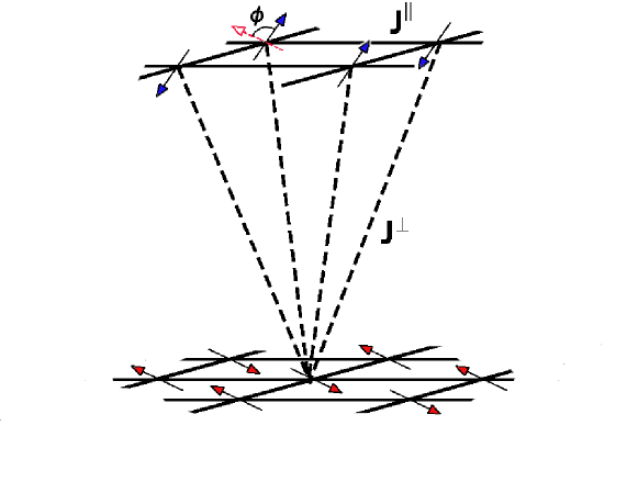
Figure 1: Lattice Structure.

To illustrate the main points of our argument, consider two separate layers of Heisenberg spins. At $T=0$ each layer is antiferromagnetically ordered, and spin waves run along the layers. Now consider the effect of a small frustrated interlayer coupling. In a system of classical spins, the layers remain decoupled in the classical ground state, and their spins may be rotated independently. The long-wavelength spin waves continue to run along the layers, and the spin fluid is quasi-two-dimensional at long wavelengths.

In the quantum-mechanical picture, even a small interlayer coupling enables magnons to virtually tunnel between layers. An antiferromagnet can be regarded as a long-range RVB state Doucot , so individual magnon transfer is energetically unfavorable, and the transfer of magnons between the layers tends to occur in pairs, as in Josephson tunneling (see Fig. 2). Interlayer magnon pair tunneling is ubiquitous in three-dimensional spin systems, frustrated and unfrustrated alike. So unless the interlayer coupling constant is set exactly to zero, magnons travel between the layers, producing a coupling closely analogous to Josephson coupling of superconducting layers. Such a coupling is an alternative way of viewing the phenomenon of “order from disorder” Henley ; Shender , whereby the free energy of zero-point or thermal fluctuations depends on the relative orientation of the classical magnetization.

If we use the analogy between superconductors and antiferromagnets, then spin rotations of an antiferromagnet map onto gauge transformations of the electron phase in a superconductor. In a superconducting tunnel junction, the Josephson energy is determined by the product of the order parameters in the two layers, i.e.

$$\Delta E_{J}\sim-\frac{t_{\perp}^{2}}{\Delta}{\rm Re}\left[\langle\psi^{\dagger}_{2\uparrow}\psi^{\dagger}_{2\downarrow}\rangle\langle\psi_{1\uparrow}\psi^{\dagger}_{1\downarrow}\rangle\right]\propto\cos(\phi_{2}-\phi_{1})$$

where $t_{\perp}$ is the tunneling matrix element, $\Delta$ the superconducting gap energy and $\psi_{l\sigma}$ ($l=1,2$) represents an electron field in lead one and two. By analogy, in a corresponding “spin junction”, the coupling energy is determined by the product of the spin-pair amplitudes. Suppose for simplicity that the system is an easy-plane XY magnet, then

$$\Delta E_{S}(\Delta\phi)\sim-\frac{J_{\perp}^{2}}{J_{\parallel}}{\rm Re}\left[\langle S^{+}_{2}(i)S^{+}_{2}(j)\rangle\langle S^{-}_{1}(i^{\prime})S^{-}_{1}(j^{\prime})\right]\propto-\frac{J_{\perp}^{2}}{J_{\parallel}}\cos(2\Delta\phi),$$

where $S^{\pm}_{li}$ represents the spin raising, or lowering operator at site $i$ in plane $l$, parallel to the local magnetization. The factor $2\Delta\phi$ arises because the spin-pair carries a phase which is twice the angular displacement of the magnetization ($S_{+}\equiv S_{x}+iS_{y}\sim Se^{i\phi}$). In other words,

$$\Delta E_{S}(\Delta\phi)\sim-\frac{J_{\perp}^{2}}{2J_{\parallel}}\cos^{2}(\Delta\phi)+\hbox{const},$$

so the interlayer coupling induced by spin tunneling is expected to be biquadratic in the relative angle between the spins. Clearly, this is a much oversimplified argument. We need to take account of the $O(3)$, rather than the $U(1)$ symmetry of a Heisenberg system. Nevertheless, this simple argument captures the spirit of the coupling between spin layers, as we shall now see in a more detailed calculation.

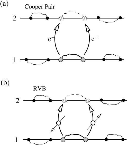
Figure 2: Contrasting (a) Josephson tunneling between paired superconductors and (b) magnon tunneling between antiferromagnets, viewed within a resonating valence bond (RVB) picture.

II Spin-Wave Spectrum for Decoupled Layers

Consider a Heisenberg model with nearest-neighbor antiferromagnetic interaction in its ground state defined on the body-centered tetragonal lattice. This choice of model is motivated by the structure of $CePd_{2}Si_{2}$, one of the compounds for which the idea of quasi-two-dimensionality was originally proposed Mathur . In this lattice structure (Fig. 1), square lattices stack with a shift of ($\frac{a}{2}$, $\frac{a}{2}$) between adjacent layers ($a$ is the lattice constant within the layer). For simplicity, the distance between the layers is also $a$. The spins of the nearest neighbors in each layer are anti-parallel. In the classical ground state the spins in different layers are decoupled and may assume any relative alignment.

For simplicity, let us consider just two adjacent layers, the argument being easily generalized to an infinite number of layers. The Hamiltonian is then

$$H=H_{0}+V,$$ (1)

with

$$H_{0}=H^{(B)}+H^{(T)},$$ (2)

where $H^{(T)}$ and $H^{(B)}$ are the Hamiltonians for the top and bottom layers, and $V$ is the interlayer coupling.

$$H_{0}=J^{\|}\sum_{\bf i,\Delta}\Bigl{(}{\bf S}_{\bf i}^{(B)}{\bf S}_{\bf i+\Delta}^{(B)}+{\bf S}_{\bf i+\delta}^{(T)}{\bf S}_{\bf i+\delta+\Delta}^{(T)}\Bigr{)},\\$$ (3)

$$V=J^{\perp}\sum_{\bf i,\Delta}\Bigl{(}{\bf S}_{\bf i}^{(B)}{\bf S}_{\bf i\pm\delta}^{(T)}+{\bf S}_{\bf i}^{(B)}{\bf S}_{\bf i+\delta-\Delta}^{(T)}\Bigr{)}.$$ (4)

Here ${\bf S}_{\bf i}^{(B)}$ (${\bf S}_{\bf i}^{(T)}$) is the spin variable defined at the site ${\bf i}$ in the bottom (top) layer. The vector ${\bf\Delta}$ denotes a displacement to the nearest neighbor sites within the plane, ${\bf\Delta}=(a,0)$ or $(0,a)$. ${\bf\delta}=(a/2,a/2)$ defines a shift between layers. Since the coupling between layers is small ($J^{\perp}\ll J^{\|}$), we may treat this model using perturbation theory where the ratio of coupling constants $J^{\perp}/J^{\|}$ is taken as a small parameter.

For our purposes, it is sufficient to consider a simple case with the spins lying in the planes of the 2-dimensional lattice. At sites ${\bf i}=(la,ma)$ and ${\bf i+\delta}=(la+\frac{1}{2}a,ma+\frac{1}{2}a)$ the spins are

$$S_{\bf i}^{X(B)}=S(-1)^{l+m},\;\;\;S_{\bf i}^{Y(B)}=0;$$ (5)

$$S_{\bf i+\delta}^{X(T)}=S(-1)^{l+m+1}\cos\phi,\;\;\;\;\;S_{\bf i+\delta}^{Y(T)}=S(-1)^{l+m+1}\sin\phi;$$ (6)

where $X$ and $Y$ are mutually perpendicular directions in the plane, $l$ and $m$ are integers.

Following a standard procedure Cooper ; Premi , we use the Holstein-Primakoff approximation for the spin operators to determine the spin-wave spectrum. The single-layer Hamiltonian $H^{(\alpha)}$ becomes

$$H^{(\alpha)} = -4NS^{2}J^{\|}+\sum_{\bf q}\Bigl{[}8SJ^{\|}a_{\bf q}^{+(\alpha)}a_{\bf q}^{(\alpha)}+SJ^{\|}({\bf q})[a_{\bf q}^{(\alpha)}a_{-\bf q}^{(\alpha)}+h.c.]\Bigr{]},$$ (7)

and on diagonalization the Hamiltonian $H_{0}$ for the decoupled layers can be written as

$$H_{0} = E_{0}+\sum_{\alpha=T,B}\sum_{\bf q}\omega^{\|}_{\bf q}b_{\bf q}^{+(\alpha)}b_{\bf q}^{(\alpha)}.$$ (8)

The ground state energy of the decoupled two-layer system is then

$$E_{0} = -8NS(S+1)J^{\|}+\sum_{\bf q}\omega^{\|}_{\bf q}.$$ (9)

$\omega^{\|}_{\bf q}$ defines the spectrum of spin waves propagating in each of the layers

$$\omega_{\bf q}^{\|}=4SJ^{\|}\sqrt{4-[\cos q_{\xi}a+\cos q_{\eta}a]^{2}}.$$ (10)

III Magnon Pair Tunneling between the Layers

Now we express the perturbation $V$ in (4) in terms of $a_{\bf q}^{+(\alpha)}$, $a_{\bf q}^{(\alpha)}$ as

$$V=S\sum_{\bf q}A^{\perp}_{\bf q}(a_{\bf q}^{+(T)}a_{\bf q}^{(B)}+h.c.)+S\sum_{\bf q}B^{\perp}_{\bf q}(a_{\bf q}^{(T)}a_{-\bf q}^{(B)}+h.c.),$$ (11)

where $A^{\perp}_{\bf q}$ and $B^{\perp}_{\bf q}$ are defined as

$$A^{\perp}_{\bf q}=2J^{\perp}\Bigl{[}\cos(\frac{q_{\xi}a}{2})\cos(\frac{q_{\eta}a}{2})+\sin(\frac{q_{\xi}a}{2})\sin(\frac{q_{\eta}a}{2})\cos\phi\Bigr{]},$$ (12)

$$B^{\perp}_{\bf q}=2J^{\perp}\Bigl{[}\cos(\frac{q_{\xi}a}{2})\cos(\frac{q_{\eta}a}{2})-\sin(\frac{q_{\xi}a}{2})\sin(\frac{q_{\eta}a}{2})\cos\phi\Bigr{]}.$$ (13)

In terms of $b_{\bf q}^{+(\alpha)}$, $b_{\bf q}^{(\alpha)}$

$$V = S\sum_{\bf q}\alpha_{q}(b_{\bf q}^{(T)}b_{-\bf q}^{(B)}+b_{\bf q}^{+(T)}b_{-\bf q}^{+(B)})+V_{ph},$$ (14)

where $\alpha_{q}=(A^{\perp}_{\bf q}\sinh 2u_{\bf q}+B^{\perp}_{\bf q}\cosh 2u_{\bf q})$ describes the amplitude for magnon pair tunneling, and $V_{ph}=S\sum_{\bf q}(A^{\perp}_{\bf q}\cosh 2u_{\bf q}+B^{\perp}_{\bf q}\sinh 2u_{\bf q})(b_{\bf q}^{+(T)}b_{\bf q}^{(B)}+b_{\bf q}^{+(B)}b_{\bf q}^{(T)})$ describes single magnon tunneling between layers.

It is straightforward to see that the particle-hole terms do not affect the ground-state energy, for $V_{ph}|GS>=0$, where $|GS>$ denotes the ground state wave-function of the system. The second order correction to the ground state energy $E_{0}$ is then

$$\Delta E_{0}^{(2)}=\sum_{\lambda}\frac{|<\lambda|\hat{V}|GS>|^{2}}{E_{\lambda}-E_{GS}},$$ (15)

where $|\lambda>$ denotes a state with two magnons being transfered between layers. Thus,

$$\Delta E_{0}^{(2)}=-\sum_{\bf q}S^{2}\alpha_{q}^{2}/(2\omega_{\bf q}^{\|}).$$ (16)

To understand the nature of coupling between the layers (dipolar or quadrupolar), let us retrive the dependence of $\Delta E_{0}^{(2)}$ on the angle $\phi$.

$$\Delta E_{0}^{(2)} = -\frac{S}{2}\frac{(J^{\perp})^{2}}{J^{\|}}[C_{0}+C_{2}\cos^{2}\phi]=$$ (17)

$$= -\frac{S}{2}\frac{(J^{\perp})^{2}}{J^{\|}}[(C_{0}+\frac{C_{2}}{2})+\frac{C_{2}}{2}\cos 2\phi].$$

The particular form of the coefficients is

$$C_{0}=\int\limits_{-\pi}^{\pi}\frac{dx\;dy}{(2\pi)^{2}}\sqrt{1-\frac{1}{4}[\cos x+\cos y]^{2}}\cos^{2}\frac{x}{2}\cos^{2}\frac{y}{2}\bigl{(}1-\frac{1}{2}[\cos x+\cos y]\bigr{)}^{2},$$ (18)

$$C_{2}=\int\limits_{-\pi}^{\pi}\frac{dx\;dy}{(2\pi)^{2}}\sqrt{1-\frac{1}{4}[\cos x+\cos y]^{2}}\cos^{2}\phi\sin^{2}\frac{x}{2}\sin^{2}\frac{y}{2}\bigl{(}1+\frac{1}{2}[\cos x+\cos y]\bigr{)}^{2}.$$ (19)

The interlayer coupling is indeed quadrupolar in nature, as foreseen earlier. Moreover, there is no small parameter, and for small S, when $J^{\perp}\sim J^{\|}$, this coupling is not weak.

IV Discussion

In the above calculation, we considered an ordered Heisenberg antiferromagnet at zero temperature. In practice, provided the spin-spin correlation length $\xi$ is large compared with the lattice constant $a$, $\xi\gg a$, a biquadratic interlayer coupling will still develop. Moreover, at finite temperatures, thermal fluctuations will produce further interlayer coupling. Both thermal and quantum interlayer coupling processes are manifestations of “order from disorder”. The main difference between the thermal and quantum coupling processes lies in the replacement of the magnon occupation numbers with a Bose-Einstein distribution function, and in general both the sign and the angular dependences of the two couplings are expected to be the same Henley . In general, geometrical frustration is an extremely fragile mechanism for decoupling spin layers and will always be overcome by quantum and thermal fluctuations. Our work was motivated by heavy electron systems. These are much more complex systems than insulating antiferromagnets, but if our mechanism for the formation of two-dimensional spin fluid is to be frustration, it is difficult to see how similar interlayer coupling effects might be avoided. We are led to conclude that for the hypothesis of the reduced dimensionality of the spin fluid in heavy fermion materials to hold, a completely different decoupling mechanism must be at work.

In the special case of XY magnetism there is, in fact, one such alternative mechanism, related to ”sliding phases”. Some heavy fermion systems, such as $YbRh_{2}Si_{2}$, are XY-like, most others, such as $CeCu_{6}$, are Ising-like. It is, therefore, instructive to consider whether the sliding phase mechanism might be generalized to Heisenberg or Ising spin systems to provide an escape from the fluctuation coupling that we have discussed.

The existence of a ”sliding phase” in weakly coupled stacks of two-dimensional (2D) XY models was predicted by O’Hern, Lubensky and Toner Lubensky . In addition to Josephson interlayer couplings, these authors included higher-order gradient couplings between the layers. In the absence of Josephson couplings, these gradient couplings preserve the decoupled nature of the spin layers, only modifying the power-law exponents of the 2D correlation functions, $\langle S_{i}S_{j}\rangle\sim r^{-\eta}$. As the temperature is raised, Josephson interlayer couplings become irrelevant above a particular ”decoupling temperature” $T_{d}$. One can always select interlayer gradient couplings to satisfy $T_{d}<T_{KT}$ and produce a stable sliding phase in the temperature window $T_{d}<T<T_{KT}$.

To see this in a little more detail, consider the continuous version of the Hamiltonian of two layers of XY models, $H=H_{0}+V$, where $H_{0}$ is a sum of independent layer Hamiltonians and $V$ is the usual Josephson-type interlayer coupling

$$H_{0}=\frac{J^{\|}}{2}\int d^{2}r[\nabla_{\perp}\phi_{T}({\bf r})]^{2}+\frac{J^{\|}}{2}\int d^{2}r[\nabla_{\perp}\phi_{B}({\bf r})]^{2},$$ (20)

$$V=J^{\perp}\int d^{2}r\cos[\phi_{T}({\bf r})-\phi_{B}({\bf r})].$$ (21)

At low temperature, when the interlayer coupling $J^{\perp}$ is zero, the average of the intralayer spin-spin correlation function with respect to $H_{0}$ is

$$\langle\phi^{2}({\bf r})\rangle_{0}=\eta\log(L/b),$$ (22)

and

$$\langle\cos[\phi({\bf r})-\phi({\bf 0})]\rangle_{0}\sim(L/b)^{-\eta},$$ (23)

where $\;\eta=T/2\pi J^{\|}$,  $L$ is the sample width and $b$ is a short-distance cutoff in the XY plane.

The average of Josephson interlayer coupling $V$ scales as ​ $\langle V\rangle_{0}\sim L^{2-\eta}$,  so Josephson couplings become irrelevant at ​ $T_{d}=4\pi J^{\|}$. ​ At temperatures above the Kosterlitz-Thouless transition temperature ​ $T_{KT}=\pi J^{\|}/2$, ​ thermally excited vortices destroy the quasi-long-range order and drive the system to disorder. In this simple example, it happens that $T_{d}>T_{KT}$,  which does not permit a sliding phase. However, higher-order gradient interlayer couplings between the layers, when added to this model, suppress $T_{d}$ below $T_{KT}$, producing a stable sliding phase for ​ $T_{d}<T<T_{KT}$.

So can the sliding phase concept be generalized to Heisenberg spin systems? A sliding phase develops in the XY model because power-law spin correlations introduce an anomalous scaling dimension, but unfortunately, a finite temperature Heisenberg model has no phases with power-law correlations Polyakov . In general, biquadratic interlayer couplings will always remain relevant in Heisenberg models. In the quantum-mechanical picture, as soon as a frustrated interlayer coupling is introduced, the order-from-disorder phenomenon Henley ; Shender generates a coupling ​ $\lambda\sim SJ^{\perp 2}/J^{\|}$ ​ between the layers:

$$H=\int\frac{\rho}{2}\sum_{i}(\nabla\hat{n}_{i})^{2}+\frac{\lambda}{2}\sum_{i}(\hat{n}_{i}-\hat{n}_{i+1})^{2},$$ (24)

where ​ $\rho=S^{2}a^{2}J^{\|}$. ​ This coupling gives us a length scale $l_{0}$ determined from ​ $(l_{0})^{-2}\sim\lambda/\rho$ ​ or ​ $l_{0}\sim a\sqrt{S}J^{\|}/J^{\perp}$. ​ Once the spin correlation length ​ $\xi\sim a\exp(2\pi J^{\|}S^{2}/T)$ ​ within a layer grows to become larger than $l_{0}$,   i.e. ​ $l_{0}<a\exp(2\pi J^{\|}S^{2}/T)$,   a ​ 3D-ordering phase transition occurs. An estimate of the 3D-ordering transition temperature is then $T_{c}\sim 2\pi J^{\|}S^{2}/\ln(\sqrt{S}J^{\|}/J^{\perp})$. ​ The answer is essentially identical in the classical picture, for here, thermal fluctuations generate an entropic interlayer coupling  $\lambda\sim\hbox{max}(SJ^{\perp 2}/J^{\|},~{}TS^{2})$,   so at high enough temperatures, for large S,   $\lambda\sim TJ^{\perp 2}/J^{\|2}$,   $l_{0}\sim SaJ^{\|~{}3/2}/J^{\perp}\sqrt{T}$. ​ A classical estimate of the 3D-ordering temperature is  $T_{c}\sim 2\pi J^{\|}S^{2}/\ln(J^{\|}/J^{\perp})$.

Another interesting question is whether XY models permit sliding phases at $T=0$. The decoupling temperature, as found by O’Hern, Lubensky and Toner Lubensky , is

$$T_{d}(p)=\dfrac{4\pi\rho}{f_{o}^{-1}-f_{p}^{-1}}.$$ (25)

One sees no obvious mechanism of suppressing $T_{d}$ to zero. A 2D sliding phase is equivalent to a 3D finite temperature sliding phase, so the existence of a sliding phase in the XY model at zero temperature would mean a power-law phase in 3D XY model. Since no power-law phase exists in 3D XY-like systems, sliding phases at $T=0$ are extremely unlikely. In conclusion, the sliding phase scenario also fails to provide a valid general mechanism for decoupling layers in Ising-like and Heisenberg-like systems.

Let us return momentarily to consider the implications of these conclusions for the more complex case of heavy electron materials. It is clear from our discussion that simple models of frustration do not provide a viable mechanism for decoupling spin layers. One of the obvious distinctions between an insulating and a metallic antiferromagnet is the presence of dissipation which acts on the spin fluctuations. The interlayer coupling we considered here relies on short-wavelength spin fluctuations, and these are the ones that are most heavily damped in a metal. Our exclusion of such effects does hold open a small possibility that order-from-disorder effects might be substantially weaker in a metallic antiferromagnet. However, if we are to take this route, then we can certainly no longer appeal to the analogy of the insulating antiferromagnet while discussing a possible mechanism for decoupling spin layers.

This research is supported by the National Science Foundation grant NSF DMR 0312495. We should particularly like to thank Tom Lubensky for a discussion relating to the sliding phases of XY antiferromagnets.

References

- (1) O. Stockert, H.v. Loehneysen, A. Rosch, N. Pyka, and M. Loewenhaupt, Phys. Rev. Lett. 80, 5627 (1998).
- (2) Q. Si, S. Rabello, K. Ingersent, and J. Smith, Nature 413, 804 (2001).
- (3) I. Paul and G. Kotliar, Phys. Rev. B 64, 184414 (2001).
- (4) N.D. Mathur, F.M. Grosche, S.R. Julian, I.R. Walker, D.M. Freye, R.K.W. Haselwimmer, and G.G. Lonzarich, Nature 394, 39 (1998).
- (5) J.A. Hertz, Phys. Rev. B 14, 1165 (1976).
- (6) T. Moriya and J. Kawabata, J. Phys. Soc. Japan 34, 639 (1973).
- (7) A.J. Millis, Phys. Rev. B 48, 7183 (1993).
- (8) P. Coleman, C. Pepin, Q. Si, R. Ramazashvili, J. Phys. Condens. Matter 13, R723 (2001).
- (9) C.L. Henley, Phys. Rev. Lett. 62, 2056 (1989).
- (10) E. Shender, Sov. Phys. JETP 56, 178 (1982).
- (11) S. Liang, B. Doucot, and P.W. Anderson, Phys. Rev. Lett. 61, 3650 (1988).
- (12) B.R. Cooper, R.J. Elliott, S.J. Nettel, and H. Suhl, Phys. Rev. 127, 57 (1962).
- (13) P. Chandra, P. Coleman, A.I. Larkin, Journal of Condensed Matter Physics 2, 7933 (1990).
- (14) C.S. O’Hern, T.C. Lubensky, and J. Toner, Phys. Rev. Lett. 83, 2745 (1999).
- (15) A. M. Polyakov, Phys. Lett. 59B, 97 (1975).
- (16) H.v. Loehneysen et al., Phys. Rev. Lett. 72, 3262 (1994).
- (17) N. Doiron-Leynaud et al., Nature 425, 595 (2003).
- (18) R.B. Laughlin, G.G. Lonzarich, P. Monthoux, D. Pines, Adv. Phys. 50, 361 (2001).
- (19) J. Custers et al., Nature 424, 524 (2003).
- (20) T. Senthil, A. Vishwanath, J. Balents, S. Sachdev, M. Fisher, Science 303, 1490 (2004).
- (21) G.R. Stewart, Rev. Mod. Phys. 73, 797 (2001).
- (22) ”A New Layered Heavy Fermion Ferromagnet, ”, D. Sokolow, M.C. Aronson, Z. Fisk, J. Chan, and J. Millican, Phys. Rev. B (submitted).
- (23) A. Schroeder et al., Nature 407, 351 (2000).
- (24) S.R. Julian et al., J. Phys. Cond. Mat. 8, 9675 (1996).
- (25) F. Steglich et al., Z. Phys. B 103, 235 (1997).
- (26) D. Belitz, T.R. Kirkpatrick, J. Rollbuehler, Phys. Rev. Lett. 93, 155701/1-4 (2004).
- (27) A. Rosch, Phys. Rev. Lett. 82, 4280 (1999).