Spin waves in paramagnetic BCC iron: spin dynamics simulations

Abstract

Large scale computer simulations are used to elucidate a longstanding controversy regarding the existence, or otherwise, of spin waves in paramagnetic BCC iron. Spin dynamics simulations of the dynamic structure factor of a Heisenberg model of Fe with first principles interactions reveal that well defined peaks persist far above Curie temperature $T_{c}$. At large wave vectors these peaks can be ascribed to propagating spin waves, at small wave vectors the peaks correspond to over-damped spin waves. Paradoxically, spin wave excitations exist despite only limited magnetic short-range order at and above $T_{c}$.

For over three decades, the nature of magnetic excitations in ferromagnetic materials above the Curie temperature $T_{c}$ has been a matter of controversy amongst experimentalists and theorists alike. Early neutron scattering experiments on iron suggested that spin waves were renormalized to zero at $T_{c}$ Collins et al. (1969); however, in 1975, using unpolarized neutron scattering techniques, Lynn at Oak Ridge (ORNL) reported Lynn (1975) that spin waves in iron persisted as excitations up to the highest temperature measured ($1.4T_{c}$), and no further renormalization of the dispersion relation was observed above $T_{c}$.

Experimentally, it was challenged primarily by Shirane and collaborators at Brookhaven (BNL) Wicksted et al. (1984a). Using polarized neutrons, they reported that spin wave modes were not present above $T_{c}$ and suggested that the ORNL group needed polarized neutrons to subtract the background scattering properly. Utilizing full polarization analysis techniques the ORNL group subsequently confirmed their earlier work and, in addition, they analyzed data from both groups and concluded that their resolution was more than an order of magnitude better than that employed by the BNL researchers Mook and Lynn (1985). Moreover, angle-resolved photoemission studies Haines et al. (1985a); Kisker et al. (1985) suggested the existence of magnetic short-range order (SRO) in paramagnetic iron and that this could give rise to propagating modes. Theoretically, SRO of rather long length scales (25 Å) was postulated to exist far above $T_{c}$ Korenman et al. (1977); Capellmann (1979a) and a more subtle kind was proposed later Heine and Joynt (1988). Contrarily, it was also suggested that above $T_{c}$, all thermal excitations are dissipative Hubbard (1979); Moriya (1991). To further complicate matters, analytical calculations for a Heisenberg model of iron, with exchange interactions extending to fifth-nearest neighbors and a three pole approximation Shastry et al. (1981), did not reproduce the line shape measured by either experimental group mentioned above. In addition, Shastry Shastry (1984) performed spin dynamics (SD) simulations of a nearest neighbor Heisenberg model of paramagnetic iron with $8192$ spins and showed some plots of dynamic structure factor $S({\bf q},\omega)$ with a shoulder at nonzero $\omega$ for some ${\bf q}$. It was explained to be due to statistical errors instead of propagating modes.

With new algorithmic and computational capabilities, qualitatively more accurate SD simulations can now be performed. In particular, it can follow many more spins for much longer integration time. We use these techniques and a model designed specifically to emulate BCC iron and have been able to unequivocally identify propagating spin wave modes in the paramagnetic state, lending substantial support to Lynn’s Lynn (1975) experimental findings. Interestingly, spin waves are found despite only limited magnetic SRO.

To describe the high temperature dynamics we use a classical Heisenberg model ${\cal H}=-(1/2)\sum_{\bf r\neq\bf r^{\prime}}J_{\bf r,\bf r^{\prime}}{\bf S}_{\bf r}\cdot{\bf S}_{\bf r^{\prime}}$, for which the exchange interactions, $J_{\bf r,\bf r^{\prime}}$, are obtained from first principles electronic structure calculations. For Fe this is a reasonable approximation since the size of the magnetic moments associated with individual Fe-sites are only weakly dependent on the magnetic state Pindor (1983) and by including interactions up to fourth nearest neighbors it is possible to obtain a reasonably good $T_{c}$.

Large scale computer simulations using SD techniques to study the dynamic properties of Heisenberg ferromagnets Chen and Landau (1994) and antiferromagnets Tsai et al. (2000) have been quite effective, and the direct comparison of RbMnF₃ SD simulations with experiments was especially satisfying Tsai et al. (2000). We have adopted these techniques and used $L\times L\times L$ BCC lattices with periodic boundary conditions and $L=32$ and 40. At each lattice site, there is a three-dimensional classical spin of unit length (we absorb spin moments into the definition of the interaction parameters) and each spin has a total of $50$ interacting neighbors. We use interaction parameters, $J_{i}$, for the $T=0$ ferromagnetic state of BCC Fe calculated using the standard formulation Liechenstein (1987) and the layer-KKR method Schulthess (1998). The calculated values are $J_{1}=36.3386$ meV, $J_{2}=20.6520$ meV, $J_{3}=-1.625962$ meV, and $J_{4}=-2.39650$ meV.

In our simulations, a hybrid Monte Carlo method was used to study the static properties and to generate equilibrium configurations as initial states for integrating the coupled equations of motion of SD Peczak and Landau (1993). At $T_{c}$ and for $L=32$, the measured nonlinear relaxation time in the equilibrating process and the linear relaxation time between equilibrated states for the total energy and for the magnetization Landau and Binder (2000) are both smaller than $500$ hybrid steps per spin. We discarded $5000$ hybrid steps (for equilibration) and used every $5000^{th}$ hybrid step’s state as an initial state for the SD simulations. For the $J_{i}$’s used here, $T_{c}=919(1)K$, which is slightly smaller than the experimental value $T_{c}^{exp}=1043K$. The equilibrium magnetization $|{\bf m}|\equiv(1/N)|\sum_{\bf r}{\bf S}_{\bf r}|\sim(1-T/T_{c})^{1/3}$ in the vicinity of $T_{c}$ and this is in agreement with experiments.

The SD equations of motion are

$$\frac{d{\bf S}_{\bf r}}{dt}={\bf H}_{eff}\times{\bf S_{\bf r}},$$ (1)

where ${\bf H}_{eff}\equiv-\sum_{\bf r^{\prime}}J_{\bf r,\bf r^{\prime}}\bf S_{\bf r^{\prime}}$ is an effective field at site ${\bf r}$ due to its interacting neighbors. The integration of the equations determines the time dependence of each spin and was carried out using an algorithm based on second-order Suzuki-Trotter decompositions of exponential operators as described in Krech et al. (1998). The algorithm views each spin as undergoing Larmor precession around its effective field ${\bf H}_{eff}$, which is itself changing with time. To deal with the fact that we are considering four shells of interacting neighbors, the BCC lattice is decomposed into sixteen sublattices. This algorithm allows time steps as large as $\delta t=0.05$ (in units of $t_{0}=J_{1}^{-1}$). Typically, the integration was carried out to $t_{max}=20000\delta t=1000t_{0}$.

The space- and time-displaced spin-spin correlation function $C^{k}({\bf r}-{\bf r^{\prime}},t)$ and the related dynamical structure factor, $S^{k}({\bf q},\omega)$, are fundamental in the study of spin dynamics Lovesey (1984) and are defined as

$$C^{k}({\bf r}-{\bf r^{\prime}},t)=\langle{S_{{\bf r}}}^{k}(t){S_{{\bf r^{\prime}}}}^{k}(0)\rangle-\langle{S_{{\bf r}}}^{k}(t)\rangle\langle{S_{{\bf r^{\prime}}}}^{k}(0)\rangle,$$ (2)

where $k=x$, $y$ or $z$ and the angle brackets $\langle\cdots\rangle$ denote the ensemble average, and

$$S^{k}({\bf q},\omega)=\sum_{{\bf r,r^{\prime}}}e^{i{\bf q}\cdot({\bf r}-{\bf r^{\prime}})}\int_{-\infty}^{+\infty}e^{i\omega t}C^{k}({\bf r}-{\bf r^{\prime}},t)\frac{dt}{\sqrt{2\pi}},$$ (3)

where ${\bf q}$ and $\omega$ are momentum and energy ($E\propto\omega$) transfer respectively. It is $S^{k}({\bf q},\omega)$ that was probed in the neutron scattering experiments discussed earlier.

By calculating partial spin sums ‘on the fly’ Chen and Landau (1994), it is possible to calculate $S^{k}({\bf q},\omega)$ without storing a huge amount of data associated with each spin configuration. Because $L$ is finite, only a finite set of $q$ values are accessible: $q=2\pi n_{q}/(La)$ with $n_{q}=\pm 1,\pm 2,\ldots,\pm L$ for the $(q,0,0)$ and $(q,q,q)$ directions and $n_{q}=\pm 1,\pm 2,\ldots,\pm L/2$ for the $(q,q,0)$ direction. ($a$ is lattice constant.) For $T\geq T_{c}$, the ensemble average in Eq. 2 was performed using at least 2000 starting configurations. We average $S^{k}({\bf q},\omega)$ over equivalent directions and this averaged structure factor is denoted as $S({\bf q},\omega)$.

In Fig. 1 we show the frequency dependence of $S({\bf q},\omega)$ obtained for four different temperatures around $T_{c}$.

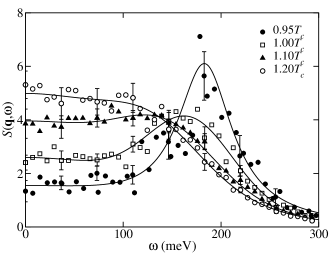
Figure 1: Calculated energy dependence of $S({\bf q},\omega)$ at ${\bf q}=\pi/a(1,0,0)$ and for $T=0.95T_{c}$ (700 runs), $1.0T_{c}$ (2000 runs), $1.1T_{c}$ (2240 runs), and $1.2T_{c}$ (2240 runs) for $L=32$. The solid lines are fits to the data as explained in text. Error bars are shown at a few typical points.

These, so called, constant-$\bf q$ scans are for ${\bf q}=\pi/a(1,0,0)$ ($|{\bf q}|=1.09$ Å^-1), which is half way to Brillouin Zone boundary. At $0.95T_{c}$, $S({\bf q},\omega)$ already has a 3-peak structure: one weak central peak at zero energy and two symmetric spin wave peaks (we only show data for $\omega\geq 0$ since the structure factor is symmetric about $\omega=0$). Note that the spin wave peaks are already quite wide. As $T$ goes to $T_{c}$ and above, the central peak becomes more pronounced. In addition, the spin wave peaks shift to lower energies, broaden further and become less obvious, however they still persist. This 3-peak structure at high temperatures is in contrast to the 2-peak spin wave structure found at low temperatures. In the neutron scattering from ⁵⁴Fe($12\%$Si) experiments Mook and Lynn (1985), Mook and Lynn also noticed a central peak, but could not decide whether it was intrinsic to pure iron or a result of alloying of silicon.

In general, constant-q scans are isotropic in the $(q,0,0)$, $(q,q,0)$, and $(q,q,q)$ directions. For very small $|{\bf q}|$, there is only a central peak in the scans (as is expected) and the 3-peak structure only develops for larger $|{\bf q}|$. We fit the 3 peaks in $S({\bf q},\omega)$ using different fitting functions and found the best results with either a Gaussian central peak plus two Lorentzian peaks at $\pm\omega_{0}$:

$$S({\bf q},\omega)=G+L_{+}+L_{-},$$ (4)

or a Gaussian central peak plus two additional Gaussian peaks at $\pm\omega_{0}$:

$$S({\bf q},\omega)=G+G_{+}+G_{-},$$ (5)

where $G=I_{c}exp(-\omega^{2}/\omega_{c}^{2})$, $L_{\pm}=I_{0}\omega_{1}^{2}/((\omega\mp\omega_{0})^{2}+\omega_{1}^{2})$, and $G_{\pm}=I_{0}exp(-(\omega\mp\omega_{0})^{2}/\omega_{1}^{2})$. For moderate $|{\bf q}|$ the results are fit best with Eq. 4, while Eq. 5 works better at larger $|{\bf q}|$.

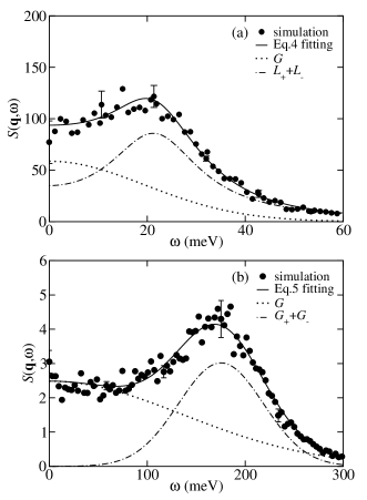
Figure 2: Fits to $S({\bf q},\omega)$ at $T=T_{c}$ for two $|{\bf q}|$-points along the $(q,q,0)$ direction for $L=32$. (a) $|{\bf q}|=0.48$ Å^-1 fit to Eq. 4, with $I_{c}=58.7$, $\omega_{c}=27.6$ meV, $I_{0}=80.6$, $\omega_{0}=21.4$ meV, and $\omega_{1}=11.3$ meV; (b) $|{\bf q}|=1.16$ Å^-1 fit to Eq. 5 with $I_{c}=2.49$, $\omega_{c}=193.3$ meV, $I_{0}=3.02$, $\omega_{0}=175.3$ meV, and $\omega_{1}=61.2$ meV. The vertical scale in (b) is much smaller than that in (a). Error bars are shown at a few typical points.

In Fig. 2 we show, for $T=T_{c}$, the results of fitting constant-${\bf q}$ scans at $|{\bf q}|=0.48$ Å^-1 and $|{\bf q}|=1.16$ Å^-1 in the $(q,q,0)$ direction. The $|{\bf q}|=0.48$ Å^-1 result fits well to Eq. 4 and has $\omega_{1}/\omega_{0}<1$, i.e., the excitation lifetime is longer than its period and thus it can be regarded as a spin wave excitation. It should be noted that this $|{\bf q}|$ value is very close to that ($0.47$ Å^-1) for which Lynn found propagating modes in contradiction to the findings of the BNL group. At $|{\bf q}|=1.16$ Å^-1, the structure factor has much weaker intensity and fits best to Eq. 5 with a ratio $\omega_{1}/\omega_{0}$ that is even smaller than at $|{\bf q}|=0.48$ Å^-1. This is illustrative of the general conclusion that the propagating nature of the excitation modes is most pronounced at large $|{\bf q}|$.

Figure 3 shows the dispersion relations obtained by plotting the peak positions, $\omega_{0}$, determined from the fits to $S({\bf q},\omega)$ along the $(q,q,0)$ direction. Calculated dispersion curves are shown at several temperatures in the ferromagnetic and paramagnetic phases together with the experimental results of Lynn Lynn (1975).

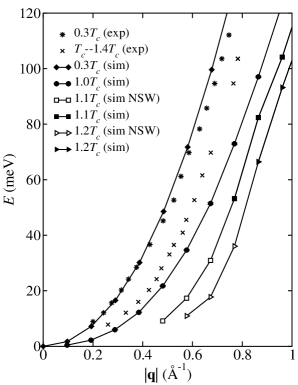
Figure 3: Comparison of dispersion curves obtained in our simulations (sim) with Lynn’s experimental (exp) (Ref. Lynn (1975)) results for the $(q,q,0)$ direction. Open symbols indicate excitations with mixed nature and are not due to spin waves (NSW).

To estimate errors, we fitted each constant-${\bf q}$ scan several times by cutting off the tail at slightly different $\omega_{max}$ to get an average $\omega_{0}$; these error bars are found to be no larger than symbols. In this figure, filled symbols indicate modes that are clearly propagating ($\omega_{1}/\omega_{0}<1$) while open symbols indicate that, even though there are peaks at $\omega_{0}\neq 0$, the peaks have widths $\omega_{1}>\omega_{0}$. The calculated result for $T=0.3T_{c}$ is very close to that from the experiments and propagating modes exist for very small $|{\bf q}|$. For $T\geq T_{c}$, our curves lie below the experiments’s and soften with increasing temperatures, a property not seen in the experiments. One possibility deserving of further study is that our use of temperature and configuration independent exchange interactions, in particular those appropriate to the $T=0$ ferromagnetic state, breaks down at high temperatures when the spin moments are highly non-collinear.

In our simulations we have equal access to constant-${\bf q}$ scans and constant-$E$ scans; however, this is not the case in neutron scattering experiments. Because the dispersion curves of Fe are generally very steep, experimentalists usually perform constant-$E$ scans. In Fig. 4 we show constant-$E$ scans for several $E$ values at $T=1.1T_{c}$ based on simulations. Clearly, the constant-$E$ scans have two peaks (symmetric about $|{\bf q}|=0$) that become smaller and wider and shift to higher $|{\bf q}|$ as $E$ increases. Peaks in constant-$E$ scans strongly suggest that SRO persists above $T_{c}$ Korenman et al. (1977).

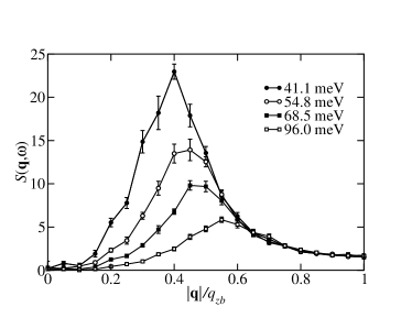
Figure 4: $T=1.1T_{c}$ constant-$E$ scans along $(q,q,0)$ direction for $E=41.1$ meV, $54.8$ meV, $68.5$ meV, and $96.0$ meV with $L=40$. Brillouin Zone boundary $q_{zb}=1.55$ Å^-1 in the direction.

The degree of magnetic SRO can be obtained directly from the behavior of static correlation function $C^{k}({\bf r}-{\bf r^{\prime}},0)$ (i.e. Eq. 2 with $t=0$), which can be calculated from the Monte Carlo configurations alone. For $T=1.1T_{c}$ we find a correlation length of approximately $2a$ ($\sim 6$ neighbor shells), indicative of only limited SRO. Thus, in general, extensive SRO is not required to support spin waves. Moreover, inspection of Fig. 3 for $T=1.1T_{c}$ shows that the point $q\gtrsim 0.77$Å^-1, at which these peaks first correspond to propagating modes, is when their wavelength ($\lambda\sim 2a$) first becomes the order of the static correlation length.

In summary, our SD simulations clearly point to the existence of spin waves in the paramagnetic state of BCC Fe and support the original conclusions of Lynn. Their signature is seen as spin wave peaks in dynamical structure factor in constant-${\bf q}$ and constant-$E$ scans. Detailed analysis of the constant-${\bf q}$ scans shows that the propagating nature of these excitations is clearest at large $|{\bf q}|$, in agreement with experiment. This is also consistent with the requirement that their wavelength be the order of, or shorter than, the static correlation length. While the inclusion of four shells of first-principles-determined interactions into the Heisenberg model makes our results specifically relate to BCC Fe, we have also found spin waves in a Heisenberg model containing only nearest neighbor interactions. In addition to elucidating the longstanding controversy regarding the existence of spin waves above $T_{c}$, these simulations also point to the important role that inelastic neutron scattering studies of the paramagnetic state can have in understanding the nature of magnetic excitations, particularly when coupled with state-of-the-art SD simulations.