Kinetics of a superconductor excited with a femtosecond optical pulse

Abstract

Superconducting state dynamics following excitation of a superconductor with a femtosecond optical pulse is studied in terms of a phenomenological Rothwarf and Taylor model. Analytical solutions for various limiting cases are obtained. The model is found to account for the intensity and temperature dependence of both photoinduced quasiparticle density, as well as pair-breaking and superconducting state recovery dynamics in conventional as well as cuprate superconductors.

In recent years numerous studies of non-equilibrium carrier dynamics in superconductors (SC) have been performed utilizing femtosecond real-time techniques [1-18]. Research focused on the identification of relaxation processes and direct measurements of the relaxation times. One of the open issues at the moment is whether cuprates are in the so called phonon bottleneck regime as conventional SCsescape , or in the weak bottleneck regime, where relaxation is governed by the biparticle recombination kinetics mercury ; orenstein ; Kaindl . The theoretical model that has been most commonly used to interpret the dynamics is a phenomenological Rothwarf-Taylor (RT) model which describes the evolution of quasiparticle (QP) and high frequency phonon (HFP) populations via a set of two non-linear differential equationsroth , which were shown recentlyovchkres to follow from the general set of kinetic equations for a SCeliash . While the RT model has been known for almost 40 years, no rigorous attempt to solve it has been made thus far, and neither has a comparison to the experimental data been made.

In this Letter we present a detailed study of the evolution of the SC state following excitation by ultrashort laser pulse using the RT model. We have obtained analytical solutions of the model in the limit of a strong and a weak bottleneck, which are in excellent agreement with numerical simulations. The solutions enable comparison of the model to the experimental results. We show that RT model can account for most of the experimental observations in conventional as well as cuprate SC, and that both conventional and cuprates SCs are in the strong bottleneck regime, where SC state recovery is governed by the HFP decay dynamics.

Rothwarf and Taylor have pointed out that the phonon channel should be considered when studying the SC relaxationroth . When two QPs with energies $\geq\Delta$, where $\Delta$ is the SC gap, recombine a HFP ($\omega>2\Delta$) is created. Since HFP can subsequently break a Cooper pair creating two QPs the SC recovery is governed by the decay of the HFP population. The dynamics of QP and HFP populations is determined byroth :

$$dn/dt =I_{0}+\eta N-Rn^{2}$$

$$dN/dt =J_{0}-\eta N/2+Rn^{2}/2-\gamma(N-N_{T})$$ (1)

Here $n$ and $N$ are concentrations of QPs and HFPs, respectively, $\eta$ is the probability for pair-breaking by HFP absorption, and $R$ the bare QP recombination rate with the creation of a HFP. $N_{T}$ is the concentration of HFP in thermal equilibrium at temperature $T$, and $\gamma$ their decay rate. $I_{0}$ and $J_{0}$ represent the external sources of QPs and HFPs, respectively mgb2 . Physically $\gamma$ is governed by the fastest of the two processes: anharmonic decay of HFP ($\omega<2\Delta$ phonons do not have sufficient energy to break Cooper-pairs) kabanov and the diffusion of HFP into the substrate escape . While the main T-dependence in $\gamma$ appears near T_ckabanov , some T-dependence is expected at low-T as well. However, as shown in Refs.Maris ; Mihailovic this T-dependence is very weak in the temperature range of interest and we can consider $\gamma$ to be T-independent.

Since $\eta/R$ has the dimensionality of concentration we introduce dimensionless QP and HFP concentrations, $q\equiv Rn/\eta$ and $p\equiv RN/\eta$, while $\theta=\eta t$ and $\tilde{\gamma}\equiv\gamma/\eta$ are the dimensionless time and HFP decay rate, respectively. Since a femtosecond optical pulse is usually shorter than characteristic timescales of SC dynamics, $I_{0}$ and $J_{0}$ could be approximated by $\delta$-functions leading to the initial concentrations of QPs $q_{0}=Rn_{0}/\eta$ and HFP $p_{0}=RN_{0}/\eta$ mgb2 . As a result Eqs. (1) reduce to

$$dq/d\theta =p-q^{2}$$ (2)

$$dp/d\theta =-p/2+q^{2}/2-\tilde{\gamma}(p-p_{T}).$$ (3)

with the initial conditions $p(0)=p_{0}$, $q(0)=q_{0}$. Here $p_{T}=RN_{T}/\eta$ is the dimensionless concentration of HFPs in thermal equilibrium. Thermal equilibrium concentrations of HFPs and QPs ($q_{T}$) satisfy the detailed balance equation $p_{T}=q_{T}^{2}$.

We investigated various limiting cases. We refer to the situation when the photoinduced density is small $(p_{0}-p_{T}),(q_{0}-q_{T})\ll 1$ as a weak perturbation regime, while the opposite case is referred to as a strong perturbation. In case $\tilde{\gamma}\ll 1$ we have a strong bottleneck (quasi-equilibrium between QPs and HFPs is established, and SC state recovery is governed entirely by $\tilde{\gamma}$) while in the opposite case ($\tilde{\gamma}\gg 1$) SC is in a weak bottleneck regime.

It is useful to estimate the values of thermal QP and HFP concentrations and compare them with $\eta/R$. If $D(\omega)=9\nu\omega^{2}/\omega_{D}^{3}$ is the phonon density of states with $\nu$ the number of atoms per unit cell and $\omega_{D}$ the Debye energy, it follows that $N_{T}=\frac{36\nu\Delta^{2}T}{\omega_{D}^{3}}\exp(-2\Delta/k_{B}T)$. On the other hand the QP density per unit cell at temperature T is given by kabanov :

$$n_{T}\simeq N(0)\sqrt{2\pi\Delta k_{B}T}\exp(-\Delta/T).$$ (4)

Here $N(0)$ is the electronic density of states per unit cell. From $\eta/R=$ $n_{T}^{2}/N_{T}$ follows that $\eta/R=\frac{N(0)^{2}\pi\omega_{D}^{3}}{18\nu\Delta}$. Regardless of the value of $\eta/R$, it follows that the high perturbation limit is reached when the photoexcitation density is close to the density required for complete depletion of the SC state. To show this, we estimate the temperature $\widetilde{T}$ where $q_{\tilde{T}}\approx 1$ ($n_{\tilde{T}}$ $\approx\eta/R$ ). It follows that $\widetilde{T}$ $\approx\Delta/\ln(\frac{\Delta^{2}\nu E_{F}}{\omega_{D}^{3}})$; thus $n_{T}$ is comparable to $\eta/R$ only in the close vicinity of $T_{c}$.

Strong bottleneck regime. Let us consider the solution of Eqs.(2,3) for the case when $\tilde{\gamma}\ll 1$. In this case two distinct regimes can be defined: (I) prebottleneck dynamics, describing the processes on timescale much shorter than $\tilde{\gamma}^{-1}$, and (II) the SC state recovery at $\theta\geq 1/\tilde{\gamma}$.

(I) Prebottleneck dynamics describes the short timescale evolution of concentrations $p(\theta)$ and $q(\theta)$ preceding the relaxation. For such short times we can neglect the last term in Eq.(3). It leads to the conservation law $q(\theta)+2p(\theta)=q_{0}+2p_{0}$ and exact solutions for QP and HFP populations, respectively, in the pre-bottleneck regime are obtainedmgb2 :

$$q(\theta) =\left[-\frac{1}{4}-\frac{\xi^{-1}}{2}+\frac{\xi^{-1}}{1-K\exp{(-\theta/\xi)}}\right]$$ (5)

$$p(\theta) =\frac{1}{2}\left[\frac{1}{8}+\frac{\xi^{-1}}{2}+\frac{\xi^{-2}}{2}-\frac{\xi^{-1}}{1-K\exp{(-\theta/\xi)}}\right]$$ (6)

Here $\xi^{-1}=\sqrt{1/4+4p_{0}+2q_{0}}$ and $K=\frac{(4q_{0}+1)-2\xi^{-1}}{4q_{0}+1)+2\xi^{-1}}$. At times $\theta>1$ concentrations $q(\theta)$ and $p(\theta)$ reach the quasi stationary solution

$$q_{s}=\frac{1}{4}(\sqrt{1+16p_{0}+8q_{0}}-1)\text{ \ ; \ \ \ \ \ }p_{s}=q_{s}^{2}.$$ (7)

The prebottleneck dynamics depends on the initial conditions, and has two distinct regimes characterized by the parameter $K$. The regime $0<K\leq 1$ corresponds to the situation when $q_{0}>q_{s}$, and $q(\theta)$ rapidly decreases during the formation of the bottleneck - Fig. 1(a). On the other hand $-1\leq K<0$ represents the situation when $p_{0}>p_{s}$, and the QP density increases up to times $\theta\approx\tilde{\gamma}^{-1}$ - Fig. 1(b). This situation is realized in MgB₂mgb2 .

(II) Superconducting state recovery dynamics. At large times ($\theta\geq 1/\tilde{\gamma}$) right hand side in Eqs.(2,3) is determined by the HFP decay term. To describe the recovery we note that at large times the difference $q^{2}-p\approx\tilde{\gamma}(p-p_{T})$ while $p(\theta)$ and $q(\theta)$ are slowly decreasing. We introduce a function $s(\theta)=q(\theta)^{2}-p(\theta)$. Cleary $s(\theta)\ll p,q$ and is slowly decaying ($ds/d\theta\ll s$). By neglecting the derivative $ds/d\theta$ it follows from the definition of $s(\theta)$ that $2q\frac{dq}{d\theta}=\frac{dp}{d\theta}$, which simplifies Eqs.(2,3) to

$$(1+2\tilde{\gamma}+4q(\theta))\frac{dq(\theta)}{d\theta}=-2\tilde{\gamma}(q(\theta)^{2}-q_{T}^{2})\text{ \ \ .}$$ (8)

After integration, we obtain an analytical solution:

$$-2\tilde{\gamma}\theta=(2+\frac{1+2\tilde{\gamma}}{2q_{T}})\ln{[\frac{q-q_{T}}{q_{s}-q_{T}}]}+(2-\frac{1+2\tilde{\gamma}}{2q_{T}})\ln{[\frac{q+q_{T}}{q_{s}+q_{T}}]}$$ (9)

Combining solutions for prebottleneck and recovery dynamics we obtain an approximate solution for $q(\theta)$ valid over the entire time range

$$q(\theta)=q_{1}(\theta)+q_{2}(\theta)-q_{s},$$ (10)

Here $q_{1}(\theta)$ and $q_{2}(\theta)$ are determined by Eqs.(5) and (9) respectively. To illustrate that Eq.(10) describes the solutions of Eqs.(2,3) we compare the numerical solution with approximation given by Eq.(10). Fig.1 shows excellent agreement for all the limiting cases.

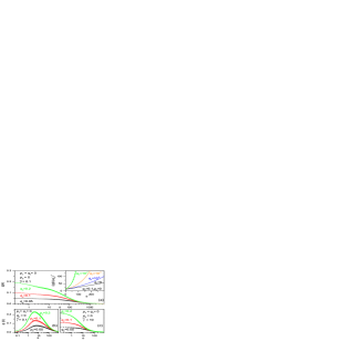
Figure 1: Analytical solutions of RT equations (open symbols) compared to numerical solutions (solid lines) in several limiting cases at $T=0$ K. Panels (a) and (b) represent the strong bottleneck limit ($\tilde{\gamma}=0.1$) for different initial conditions (see text). Analytical solution for $q(\theta)$ is given by Eq.(10). Panel (c) presents the weak bottleneck case ($\tilde{\gamma}=10$). The inset to panel (a) presents the inverse of the photoinduced QP density as a function of $\theta$ for various temperatures ($q_{T}$). At low-T ($q_{T}\longrightarrow 0$) the time dependence is linear, mimicking the bimolecular kinetics, while at higher T it becomes nearly exponential (dashed curve presents an exponential decay fit). Indeed, similar behavior was recently reported Kaindl .

Eq.(9) can be simplified in the low and high-T limits:

i) Low temperature limit $(q_{T}\ll 1).$

In this case $2\ll\frac{1+2\tilde{\gamma}}{2q_{T}}$ and Eq.(9) reduces to:

$$q(\theta)=q_{T}+\frac{2q_{T}(q_{s}-q_{T})\exp{(-\theta/\tau_{T})}}{(q_{s}+q_{T})-(q_{s}-q_{T})\exp{(-\theta/\tau_{T})}}$$ (11)

The relaxation rate $\tau_{T}^{-{1}}=4\tilde{\gamma}q_{T}/(1+2\tilde{\gamma})$ is strongly reduced by the additional T-dependent factor $q_{T}\varpropto n_{T}$. The behavior is consistent with the T-dependence of the relaxation time $\tau$ in most of the SCs: cupratemercury ; Schneider ; Segre and conventional mgb2 ; Tanner . The low-T divergence of $\tau$ was originally attributed to the bi-particle prebottleneck dynamicsmercury where $\tau$ is divergent due to strong reduction of the thermal QP density. Here we show that at low-T $\tau$ diverges also in the case of a well established bottleneck.

In the limit of $\theta/\tau_{T}\ll 1$ Eq.(11) further reduces to $q(\theta)=q_{s}/(1+\frac{2q_{s}\tilde{\gamma}\theta}{1+2\tilde{\gamma}})$, showing identical dynamics to that of the biparticle recombination - see inset to Fig. 1(a). If one defines the relaxation rate as the slope $\tau^{-1}=|dq(\theta)/d\theta|/(q_{s}-q_{T})$ at $\theta\rightarrow 0$, as proposed in Ref.orenstein , the SC relaxation rate is intensity dependent

$$\tau^{-1}=\frac{2(q_{s}+q_{T})\tilde{\gamma}}{(1+2\tilde{\gamma})}\text{.}$$ (12)

The intensity dependence is observed only if $q_{s}\gg q_{T}$; in this case $\tau^{-1}$ is proportional to the excitation intensity. It follows from Eq.(12), that the observation of pronounced intensity dependence of $\tau$ is constrained only to the very low-T (determined by the $\Delta/kT_{c}$ ratio) and is more likely to be observed in cuprates than in conventional SCs. Indeed, the intensity dependent recovery dynamics has been recently observed at low-T in BiSCOKaindl , in agreement with the solution of RT equations in the strong bottleneck regime - inset to Fig. 1(a).

ii) High temperature limit $(q_{T}\gtrsim 1).$

In this case $2\gg\frac{1+2\tilde{\gamma}}{2q_{T}}$ and Eq.(9) reduces to:

$$q(\theta)=\sqrt{q_{T}^{2}+(q_{s}^{2}-q_{T}^{2})\exp{(-\theta/\tau_{T})}}$$ (13)

Here the relaxation rate $\tau_{T}^{-1}=\tilde{\gamma}$ is weakly T-dependent (due to intrinsic T-dependence of $\tilde{\gamma}$), and does not depend on $q_{s}$ or $p_{s}$, implying that the relaxation rate is intensity independent. The same is true also for $\tau^{-1}$.

Weak bottleneck ($\tilde{\gamma}\gg 1$). In this case at short times $\theta\approx\tilde{\gamma}^{-1}\ll 1$ the last term in Eq.(3) is dominant, and the solution has the form

$$p(\theta)=p_{T}+(p_{0}-p_{T})\exp{(-\tilde{\gamma}\theta)}\text{ .}$$ (14)

The HFP density reaches its thermodynamic value on a time scale determined by $\tilde{\gamma}^{-1}$. On such a short time scale QP density has not been changed, therefore we can substitute $p$ with $p_{T}$ in Eq.(2). Taking into account that $q_{T}^{2}=p_{T}$ we obtain the solution:

$$q(\theta)=\frac{q_{T}[q_{0}+q_{T}+(q_{0}-q_{T})\exp{(-2q_{T}\theta)}]}{q_{0}+q_{T}-(q_{0}-q_{T})\exp{(-2q_{T}\theta)}}.$$ (15)

Eqs.(14,15) present the solution of Eqs.(2,3) for all timescales. As seen in Fig. 1(c) the difference between the analytical and numerical solutions is negligible. Similar to the case of a strong bottleneck the relaxation rate determined as the slope of the signal at $\theta=0$ is found to be intensity dependent if $q_{0}\gg q_{T}$ with $\tau^{-1}=(q_{0}+q_{T})$. The main difference between the strong and weak bottleneck cases is that the absolute value of $\tau^{-1}$ is in the strong bottleneck case reduced by the HFP decay time.

Photoinduced QP density. Earlier kabanov we have discussed the T and excitation intensity dependence of the photoinduced signal amplitude Q (proportional to the photoinduced QP density) assuming the bottleneck condition and the energy conservation law. These results were recently confirmed using a realistic phonon density of statesnicol . However, solution of Eqs.(2,3) allows unambiguous comparison of Q$(T)$ with the expected T-dependence in a SC - without an additional assumption of the energy conservation as in Refs.kabanov ; nicol .

In the strong bottleneck regime initial dynamics leads to the stationary densities of QPs and HFPs determined by Eqs.(7). The initial concentrations can be written as $q_{0}=q_{T}+\Delta q$ and $p_{0}=p_{T}+\Delta p$, where $\Delta q$, $\Delta p$ are photoinduced initial concentrations of QPs and HFPs, respectively. Assuming weak perturbation limit $\Delta p,$ $\Delta q\ll 1$ the amplitude of the signal is given by:

$$\emph{Q}(T)\propto q_{s}-q_{T}\approx\frac{2\Delta p+\Delta q}{4\sqrt{1+16p_{T}+8q_{T}}}$$ (16)

Taking into account that $p_{T}=q_{T}^{2}$ and $q_{T}=Rn_{T}/\eta$, and normalizing Q to its low-T value, $A=\emph{Q}/\emph{Q}_{T\rightarrow 0K}$, we obtain $n_{T}\propto A^{-1}-1$. This relation is expected to be general and valid for any SC irrespective on the gap symmetry allowing direct estimation of the T-dependence of QP density in thermal equilibrium.

Importantly, in the weak bottleneck case Q should be proportional to the pump intensity, and T-independent at low-T since $q(\theta=0)=q_{0}$, while increasing when $T\rightarrow T_{c}$ due to closing of the SC gap. This T-dependence has not been observed thus far.

In Fig. 2 we plot the T-dependences of $n_{T}$ (extracted from the raw data via $n_{T}\propto A^{-1}-1$) and the SC recovery time $\tau$ for MgB₂ and the cuprate superconductor Tl₂Ba₂CuO_6+δ. The two datasets capture the main features observed on other conventional Carr ; Tanner or cuprate kabanov ; Smith ; mercury ; THzAveritt ; Segre ; Schneider superconductors. In both Q gradually decreases upon increasing T towards T_c kabanov ; Smith ; mercury ; THzAveritt ; Segre ; Schneider ; Carr ; Tanner , while the low-T relaxation time increases when $T\longrightarrow 0$. The only exception thus far was the near optimally doped YBCO, where $\tau$ is roughly constant at low-T kabanov ; THzAveritt . The main difference between cuprates and conventional SC is a 1-2 orders of magnitude difference in $\tau$, which can be understood in terms of an order of magnitude difference in the value of the SC energy gapcomparison .

While at low-T and weak perturbations both strong and weak bottleneck scenarios suggest slowing down of the relaxation upon cooling as well as intensity dependent relaxation, the fact that the amplitude gradually decreases upon T-increase suggests that all SC studied thus far are in the strong bottleneck regime (in the weak bottleneck scenario Q should increase upon increasing T). In order to test the agreement of the model with the data, we fit $n_{T}$ with Eq.(4), where BCS form for $\Delta(T)$ was used. We find good agreement between the extracted values for $2\Delta/T_{c}$ from the fit with the values from other experimental techniquescomparison ; Tl2201gap .

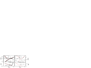
Figure 2: Comparison of the experimental data on T-dependence of $n_{T}$ and $\tau$ on a) MgB₂ mgb2 ; CarrMgB2 and b) Tl₂Ba₂CuO_6+δ Smith with the RT solution. $n_{T}$ is extracted from the raw data (shown in insets) using $n_{T}\propto A^{-1}-1$ and fit with Eq.(4), while $\tau$ was fit with Eq.(12). The extracted values of $2\Delta/T_{c}$ ratio are also shown.

We fit the T-dependence of the relaxation time $\tau$ with Eq.(12). Assuming $\tilde{\gamma}$ to be T-independent and expressing $q_{T}$ with Eq.(4), Eq.(12) is rewritten to $\tau(T)=1/(\Phi+A(\Delta T)^{1/2}\exp(-\Delta/T))$. Here $\Phi$ $=B(q_{s}-q_{T})$, while $A$ and $B$ are fitting parameters. Since the T-dependence of $q_{s}-q_{T}$ is measured directly - see Eq.(16), we are left with 3 fitting parameters: $A$, $B$ and $\Delta$. The T-dependence of $\tau$ is governed mainly by $\exp(-\Delta/T)$ term, while $A$ and $B$ account for the magnitude of $q_{T}$ and $(q_{s}-q_{T})$ respectively. At the intermediate temperatures $q_{s}-q_{T}\ll q_{T}$, and $\tau$ is governed by the T-dependence of $q_{T}$ showing $\exp(\Delta/T)$ behavior. At low enough T, however, $q_{s}\gg q_{T}$ and the relaxation time saturates. The values of $\Delta$ extracted from relaxation time data are somewhat lower than the values extracted from the fit to $n_{T}$. This can be partially attributed to the fact that the T-dependence of $\tilde{\gamma}$ was neglected. More importantly, improper (or missing) treatment of the laser heating can also cause an underestimate of $\Delta$ obtained from the fit. Namely, due to laser excitation the equilibrium T of the probed spot can be substantially higher than that of the cold fingerACS , especially at low-T. Therefore, the T-dependence of $\tau$ is not as steep as if the temperature scale was corrected for heating, giving rise to an underestimate of $\Delta$. Note that heating is particularly pronounced in experiments using high repetition rate laser systems like in Ref.Smith . Finally, we should note that the value of $\Delta$ extracted is also somewhat dependent on the T-dependence of $\Delta$, i.e. when fitting we used a BCS form. However, the accuracy of the available experimental data is not sufficient enough to speculate about the deviation of the temperature dependence from the BCS functional form.

In conclusion, we studied the evolution of a SC state following perturbation with ultrashort optical pulses. We derived analytical solutions of RT model for the strong and weak bottleneck regimes. Analytical solutions account for both pair-breaking dynamicsmgb2 as well as SC state recovery, and are in excellent agreement with numerical results. They enable comparison to experimentally measured quantities like the SC state recovery time and the photoinduced QP density. Comparison with published data suggest that both cuprate and conventional SCs follow the RT scenario, both being in the strong bottleneck regime.

We would like to acknowledge A.S. Alexandrov and T. Mertelj for critically reading the manuscript.

References

- (1) S.G. Han, et al., Phys. Rev. Lett. 65, 2708 (1990).
- (2) C.J. Stevens, et al., Phys. Rev. Lett. 78, 2212 (1997).
- (3) J. Demsar, et al., Phys. Rev. Lett. 82, 4918 (1999).
- (4) V.V. Kabanov, et al, Phys. Rev. B 59, 1497 (1999).
- (5) D.C. Smith, et al., Physica C 341, 2219 (2000).
- (6) R.D. Averitt, et al., Phys. Rev. B 63, 140502(R) (2001).
- (7) G.P. Segre, et al., Phys. Rev. Lett. 88, 137001 (2002).
- (8) M.L. Schneider, et al., Europhys. Lett. 60, 460 (2002).
- (9) J. Demsar, et al., Phys. Rev. B 63, 054519 (2001).
- (10) G.L. Carr, et al., Phys. Rev. Lett. 85, 3001 (2000).
- (11) J.F. Federici, et al., Phys. Rev. B 46, 11153 (1992).
- (12) J. Demsar, et al., Phys. Rev. Lett. 91, 267002 (2003).
- (13) R.P.S.M. Lobo, et al., cond-mat/0404708.
- (14) R.P.S.M. Lobo, et al., Phys. Rev. B 72, 024510 (2005).
- (15) R.A. Kaindl, et al., Science 287, 470 (2000).
- (16) J. Demsar, et al., J. Supercond. 17, 143 (2004).
- (17) N. Gedik, et al., Phys. Rev. B 70, 014504, (2004).
- (18) R.A. Kaindl, et al., CLEO/IQEC Technical Digest on CDROM, (OSA, Washington, DC, 2004), ITuF1.
- (19) A. Rothwarf, G.A. Sai-Halasz, and D.N. Langensberg, Phys. Rev. Lett. 33, 212, (1974).
- (20) A. Rothwarf and B.N. Taylor, Phys. Rev. Lett. 19, 27 (1967).
- (21) Yu.N. Ovchinnikov and V.Z. Kresin, Phys. Rev. B 58, 12416 (1998).
- (22) G.M. Eliashberg, Zh. Eksp. Theor. Fiz., 61, 1254, (1971) [Sov. Phys. JETP, 34, 668 (1971)].
- (23) S. Tamura, H.J. Maris, Phys. Rev. B 51, 2857 (1995).
- (24) D.Mihailovic, et al., Phys. Rev. B 47, 8910 (1993).
- (25) E. J. Nicol and J. P. Carbotte, Phys. Rev. B 67, 214506 (2003).
- (26) L. Ozyuzer et al., Phys. Rev. B 57, R3245 (1998).
- (27) D. Mihailovic and J. Demsar in Spectrosopy of Superconducting Materials, ed. Eric Falques, ACS Symposium Series 730; ACS, Washington, D.C., 1999.