Pseudospin ferromagnetism in double–quantum-wire systems

Abstract

We propose that a pseudospin ferromagnetic (i.e. inter-wire coherent) state can exist in a system of two parallel wires of finite width in the presence of a perpendicular magnetic field. This novel quantum many-body state appears when the inter wire distance decreases below a certain critical value which depends on the magnetic field. We determine the phase boundary of the ferromagnetic phase by analyzing the softening of the spin-mode velocity using the bosonization approach. We also discuss signatures of this state in tunneling and Coulomb drag experiments.

Ferromagnetism (FM) in low dimensional itinerant electronic systems is one of the most interesting subjects in condensed matter physics. As early as in the ’60s Lieb and Mattis lieb (LM) has proved that a ferromagnetic state cannot exist in one-dimensional (1D) system if the electron-electron interaction is spin/velocity-independent and symmetric with respect to the interchange of electron coordinates. Therefore, possible candidates for 1D FM must involve some nontrivial modification in the band structure and interaction to avoid the restrictions of LM’s theorem. Most of the examples proposed in the literature ferro_review1 rely on some highly degenerate flat bands (or at least systems with the divergent density of states) and can be understood as a generalization of Hund’s rule Hund . The only exception appears to be a model of finite range hopping with a negative tunneling energy ferro_review2 .

From the experimental point of view, however, physical realization of the 1D FM in thermodynamical limit is still absent to the best of our knowledge. In two-dimensions (2D), some of the most intriguing ferromagnetic systems are the quantum Hall (QH) bilayers at the total filling factor one. In these systems the flat band structure is provided by the magnetic field (Landau levels) and clear experimental evidence of the 2D pseudospin ferromagnetism (PSFM, with the pseudospin being the layer index) has been observed in the tunneling spielman01 and drag experiments 2d_drag_exp several years after theoretical proposals QH_review .

In this paper we propose a realistic one-dimensional system which should exhibit a pseudospin ferromagnetic order. The system consists of two finite-width quantum wires with a magnetic field applied perpendicular to the wire surface, see Fig. 1(a). In the presence of the magnetic field, single-electron states are modified, which leads to a strong effective mass enhancement and modification of the effective Coulomb interaction. These two effects can lead to a softening of the spin mode velocity when the inter-wire distance becomes smaller than a critical value $d_{c}$. The system then becomes an easy-plane PSFM state due to the appearance of interwire coherence (IWC), which should manifest itself in the appearance of the resonant peak in the tunneling conductance at small bias voltages. We also calculate the drag resistance of such 1D PSFM state within the mean-field approximation and demonstrate that the drag resistance first increases and scales with the longitudinal size as the magnetic field is increased (or the inter-wire distance is decreased) toward the phase transition boundary and then becomes dramatically reduced (i.e. not scaled with the size) when entering the PSFM state. The proposed 1D PSFM transition should be experimentally accessible by the present or near future semiconductor technology.

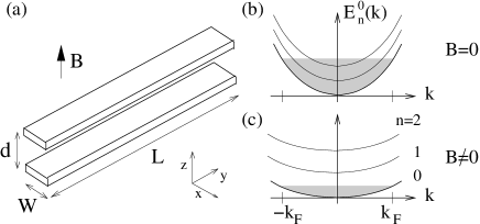
Figure 1: (a) Schematic double wire system considered in this paper. (b) and (c) are single particle energy $E^{0}_{n}(k)$ of each wire for $B=0$ and $B\neq 0$ cases respectively.

The double wire system we consider is aligned in the $y$ direction, Fig. 1(a), and centered at $x=0$ and $z=\pm d/2$. Electrons are confined by a parabolic potential, $\frac{1}{2}m\omega_{0}^{2}x^{2}$, in the $x$ direction and their motion in $z$ direction is assumed to be totally quenched. Using the Landau gauge, the single particle Hamiltonian of momentum $k$ in each wire can be derived to be

$$H_{0} = -\frac{1}{2m}\partial_{x}^{2}+\frac{1}{2}m\tilde{\omega}^{2}(x-x_{0})^{2}+\frac{k^{2}}{2m^{\ast}},$$ (1)

where $m^{\ast}=m(\omega_{c}^{2}+\omega_{0}^{2})/\omega_{0}^{2}$ is the renormalized electron mass, $\tilde{\omega}=\sqrt{\omega_{0}^{2}+\omega_{c}^{2}}$ is the Landau level splitting, and $x_{0}=l_{0}^{2}k$ is the guiding center coordinate with $l_{0}=\sqrt{\omega_{c}/m(\omega_{c}^{2}+\omega_{0}^{2})}$ being the magnetic length. $\omega_{c}=eB/mc$ is the bare cyclotron frequency. The wave-functions and energy spectrum of Eq. (1) are easily found from the analogy with the standard QH system QH_wang : $\psi_{n,k,s}({\bf r})=L^{-1/2}e^{iky}\varphi_{n}(x+x_{0})\sqrt{\delta(z-sd/2)}$ and $E_{n}^{0}(k)=(n+\frac{1}{2})\tilde{\omega}+\frac{k^{2}}{2m^{\ast}}$, where $n$ is the Landau level index and $s=\pm\frac{1}{2}$ is the pseudospin index for the upper/lower wire, $\varphi_{n}(x)=(\pi^{1/2}2^{n}n!\,\tilde{l}_{0})^{-1/2}e^{-x^{2}/2\tilde{l}_{0}^{2}}H_{n}(x/\tilde{l}_{0})$ is the $n$-th eigenfunction of a parabolic potential with $\tilde{l}_{0}\equiv\sqrt{1/m\tilde{\omega}}$. Throughout this paper we concentrate on the strong magnetic field (or low electron density) regime so that only the lowest energy level ($n=0$) is occupied. One can see that the magnetic field not only modifies the band splitting, but also increases the effective mass in the longitudinal ($y$) direction, leading to a flatband structure with high density of states similar to the Landau level degeneracy in 2D system, see Fig. 1(b).

The interaction Hamiltonian can be derived to be QH_wang :

$$H_{1} = \frac{1}{2\Omega_{\perp}}\sum_{s_{1},s_{2},k_{1},k_{2},{{\bf q}}_{\perp}}V_{s_{1},s_{2}}({{\bf q}}_{\perp},k_{1},k_{2})$$ (2)

$$\times c^{\dagger}_{s_{1},k_{1}+q_{y}/2}c_{s_{1},k_{1}-q_{y}/2}c^{\dagger}_{s_{2},k_{2}-q_{y}/2}c_{s_{2},k_{2}+q_{y}/2},$$

where $c_{s,k}(c^{\dagger}_{s,k})$ are the electron field operators, $\Omega_{\perp}=LW$ is the wire area, and $V_{s,s^{\prime}}({\bf q}_{\perp},k_{1},k_{2})=A({\bf q}_{\perp})^{2}\int\frac{dq_{z}}{2\pi}V({\bf q})\left[1+\delta_{s,-s^{\prime}}(e^{-iq_{z}d}-1)\right]\,e^{-iq_{x}(k_{1}-k_{2})l_{0}^{2}}$ is the effective 1D interaction with $V({\bf q})$ being the Coulomb interaction. The form-function, $A({{\bf q}}_{\perp})=\exp\left[-\left(q_{x}^{2}\tilde{l}_{0}^{\,2}+q_{y}^{2}l_{0}^{4}/\tilde{l}_{0}^{\,2}\right)/4\right]$ is obtained by integrating the electron spatial wave function QH_wang . Due to the presence of magnetic field, the effective 1D interaction, $V_{s,s^{\prime}}({\bf q}_{\perp},k_{1},k_{2})$, is not equivalent to any spin-independent (or velocity-independent) symmetric potential. Thus in our system, the ferromagnetic state is not inhibited by the LM’s theorem.

Figure 2: Calculated critical interlayer distance, $d_{c}$, as a function of magnetic field ($\propto\omega_{c}$). Electron density in an individual wire, $n_{e}$, is 0.6, 0.7, $\cdots$, $1.0\times 10^{5}$ cm^-1 from top to bottom. Here $\lambda_{0}=500$ Å  and $\omega_{0}=0.05$ meV.

Starting from Eqs. (1)-(2), one can use the standard bosonization approach to describe the low energy physics near the Fermi points. After neglecting the irrelevant (nonlocal) terms, we obtain $H=\sum_{a=\rho,\sigma}H_{a}+H_{b}$, where

$$H_{a} = \frac{u_{a}}{2\pi}\int dy\left[K_{a}\Pi_{a}(y)^{2}+\frac{1}{K_{a}}\partial_{y}\Phi_{a}(y)^{2}\right].$$ (3)

Here the sum consists of charge $\rho$ and spin $\sigma$ channels. $H_{b}\propto\int dy\cos(\sqrt{8}\Phi_{\sigma}(y))$ describes the undiagonalizable backward scattering term LL_review . $\Pi_{a}$ and $\Phi_{a}$ are the bosonic operators satisfying the commutation relation: $[\Phi_{a}(y),\Pi_{a^{\prime}}(y^{\prime})]=i\delta_{a,a^{\prime}}\delta(y-y^{\prime})$. The renormalized velocity and Luttinger exponents are

$$u_{a}=v_{F}\sqrt{(1+\tilde{g}_{\theta_{a}})(1+\tilde{g}_{\phi_{a}})},\ \ \ K_{a}=\sqrt{\frac{1+\tilde{g}_{\theta_{a}}}{1+\tilde{g}_{\phi_{a}}}}$$ (4)

where $\tilde{g}_{\theta_{a}/\phi_{a}}=\frac{1}{2\pi v_{F}}\left(2g_{4,a}\mp(2g_{2,a}-g_{1,\|})\right)$ and $g_{i,\rho/\sigma}\equiv\frac{1}{2}\left(g_{i,\|}\pm g_{i,\perp}\right)$. Here $g_{4,\|/\perp}=\int\frac{dq_{x}}{2\pi}\left[V_{I/O}(q_{x},0)\right]$, $g_{2,\|/\perp}=\int\frac{dq_{x}}{2\pi}V_{I/O}(q_{x},0)\cos(2q_{x}k_{F}l_{0}^{2})$, and $g_{1,\|/\perp}=\int\frac{dq_{x}}{2\pi}V_{I/O}(q_{x},2k_{F})$ are defined as the usual $g$-ology interaction in the Luttinger liquid theory LL_review with $k_{F}$ being the Fermi momentum. $V_{I}({\bf q}_{\perp})$ and $V_{O}({\bf q}_{\perp})$ are the intra-wire and inter-wire interaction matrix elements, respectively. To simplify calculations we model the screened Coulomb interaction by using $V({\bf q})=(4\pi e^{2}\lambda_{0}^{2}/\epsilon_{0})e^{-|{\bf q}|^{2}\lambda_{0}^{2}}$ where $\epsilon_{0}$ is the static dielectric constant and $\lambda_{0}$ is screening length. The qualitative results obtained below should not be sensitive to the details of the screening potential.

The ferromagnetic transition occurs as the spin stiffness, $v_{N,\sigma}=u_{\sigma}/K_{\sigma}=v_{F}(1+\tilde{g}_{\phi_{\sigma}})$, becomes zero yang , or $g_{1\|}=2\pi v_{F}+2(g_{4,\sigma}+g_{2,\sigma})$. In general the low energy Luttinger liquid parameters should be renormalized by the backward scattering, $H_{b}$, and therefore the phase boundary obtained from the bare Luttinger parameters should be modified also. However, when in PSFM phase, the spin stiffness is negative so that higher order derivatives, like $\partial_{y}^{2}\Phi_{\sigma}$, has to be included to stablize the system and to give a nonzero spin density, $\rho_{s}\propto\partial_{y}\Phi_{\sigma}$ yang . As a result, the sine-Gordon backward scattering will oscillate in real space and hence become negligible after averaging in the thermodynamical limit. Therefore for simplicity we may assume that the renormalization effects are not very serious so that the phase boundary of the PSFM state can still be estimated roughly by using the bare Luttinger parameters as stated above. The critical behavior of similar transition has been also discussed very recently yang .

In Fig.2 we show the calculated critical inter-wire distance as a function of magnetic field for various single wire electron densities, $n_{e}$. PSFM occurs in the large field and small distance regime. At zero distance, $g_{2/4,\sigma}=0$, and therefore the critical field ($\omega_{c,cr}$) is the minimum field strength for the backward interaction ($g_{1,\|}$) to be dominant. On the other hand, in the extremely large field regime, the Fermi velocity approaches zero. The critical distance ($d_{cr}$) is now determined by the competition between the backward scattering and the forward scattering in the spin channel. In large density limit ($k_{F}\lambda_{0}=\pi n_{e}\lambda_{0}>1$) we can obtain the analytic expression of $\omega_{c,cr}$ and $d_{cr}$: $\omega_{c,cr}\sim\omega_{0}\sqrt{2r_{s}^{-1}e^{(2k_{F}\lambda_{0})^{2}}-1}$ and $d_{cr}\sim\lambda_{0}e^{-(2k_{F}\lambda_{0})^{2}}$, where $r_{s}\equiv me^{2}/\epsilon_{0}\pi k_{F}$ is the ratio of the average potential and kinetic energies. We also checked explicitly that in the parameter regime we consider here the pseudospin polarized state is always energetically unfavorable compared to the (easy-plane) pseudospin ferromagnetic phase.

We now discuss how such PSFM phase can be observed in realistic experiments. In this phase the system has quasi long-range order characterized by the presence of a Goldstone mode. Tunneling spectroscopy has been used to observe similar modes in the QH bilayers spielman01 and can be also applied to the present system. We expect a strong enhancement of the tunneling conductance at small voltage bias when the system enters the PSFM state. Another approach to demonstrating the 1D PSFM in the double wire system is to perform the Coulomb drag experiments. Such experiments have been done on 2D2d_drag_exp and 1D1d_drag_exp semiconductor heterostructures in recent years, and the drag resistance, $R_{d}$, is a direct measure of the effects due to inter-wire interaction Roj . In the literature without magnetic field or interwire coherence, the drag resistance behaves differently in the two different regimes: In the perturbative regime $R_{d}$ vanishes in low temperature limit ($R_{d}\propto T^{2}\ll e^{2}/\hbar$) Roj ; drag_eugene ; in the strong interaction regime, however, the backward scattering between the two wires becomes relevant NA and opens a gap $\tilde{\Delta}$ in the energy spectrum, corresponding to the formation of a locked charge density wave phase (LCDW) with a divergent drag resistivity $R_{d}\propto\exp{(\tilde{\Delta}/T})$ in low temperature regime.

To analyze the drag resistance in the presence of inter-wire coherence, it is useful to employ the Hartree-Fock (HF) approximation. This approach neglects long wavelength fluctuations present in 1D systems, but we expect these fluctuations give rise only to small corrections in the drag resistance deep inside the PSFM phase. The HF Hamiltonian then can be easily diagonalized by transforming the electron operators into the symmetric ($c^{\dagger}_{\uparrow,k}+c^{\dagger}_{\downarrow,k}$) and the antisymmetric ($c^{\dagger}_{\uparrow,k}-c^{\dagger}_{\downarrow,k}$) channels with the eigenenergies, $E^{\pm}_{k}=k^{2}/2m^{\ast}+\Sigma_{k}\mp\Delta_{k}-W_{0}$.

Figure 3: (a) Typical setup for conductance experiment of the double wire system, where the two wires interact in the middle regime ($0<y<L$) and are connected to ideal 1D reservoir in the left ($y<0$) and right ($y>L$) hand sides. The upper (active) wire is biased by a voltage $V$, while the lower (passive) wire is biased by $V_{R}$ and $V_{L}$ with currents $I_{\uparrow/\downarrow}$ in the two wires respectively. (b) and (c) are the band energy for electrons in the incoherent reservoirs and in the coherent double wire regime respectively. The upper and lower bands in (b) are for the antisymmetric and symmetric bands respectively.

Here $\Sigma_{k}$ and $\Delta_{k}$ are the intra-wire self-energy and the IWC gap respectively, and $W_{0}$ is the shift of the band energy in response to the reconstruction of the ground state due to coupling to leads, see Fig. 3(b)-(c). For simplicity, in our calculation we neglect the momentum dependenace of $\Sigma_{k}$ and $\Delta_{k}$ and approximate them by their values at $k=0$. Within this approximation, we obtain (at zero temperature):

$$\Sigma_{0} \sim \frac{V_{1}n_{\rm coh}}{4}(1+e^{-(d/2\lambda_{0})^{2}})-\frac{V_{1}}{8\sqrt{\pi}\lambda_{y}},$$ (5)

$$\Delta_{0} \sim \frac{V_{1}e^{-(d/2\lambda_{0})^{2}}}{8\sqrt{\pi}\lambda_{y}}$$ (6)

where $V_{1}\equiv e^{2}\lambda_{0}/\epsilon_{0}\lambda_{x}$, $\lambda_{x}\equiv\sqrt{\lambda_{0}^{2}+\tilde{l}_{0}^{2}/4}$, and $\lambda_{y}\equiv\sqrt{\lambda_{0}^{2}+l_{0}^{4}/\tilde{l}_{0}^{2}}$. $n_{\rm coh}=2n_{e}$ is the total electron density of both wires in the coherent regime. In above equations, we have assumed that all electrons fall into symmetric band. This is justified because the bottom of the antisymmetric band can be shown to be above the chemical potential by $\Delta E=2\Delta_{0}-4\eta^{2}E_{F}>0$, when the magnetic field is large enough (Fermi energy $E_{F}=\frac{k_{F}^{2}}{2m^{\ast}}\propto B^{-2}$).

To calculate the drag resistance in a typical experimental setup, Fig. 3(a), we first note that the drag resistance [$R_{d}=(V_{R}-V_{L})/I_{\uparrow}$ for $I_{\downarrow}=0$] can be expressed through the conductance of symmetric currents [$G_{+}=I_{\uparrow}/V$ for $V_{L}=V$, $V_{R}=0$ and hence $I_{\uparrow}=I_{\downarrow}$] and the conductance of antisymmetric currents [$G_{-}=I_{\uparrow}/V$ for $V_{L}=0$, $V_{R}=V$ and hence $I_{\uparrow}=-I_{\downarrow}$], according to: $R_{d}=G_{-}^{-1}-G_{+}^{-1}$. The symmetric and antisymmetric conductances, $G_{\pm}$, in the presence of inter-wire coherence at temperature $T$ can be easily derived to be unpublished ,

$$\left.\begin{array}[]{c}G_{+}\\ G_{-}\end{array}\right\}=\frac{e^{2}}{16\pi T}\int\frac{dE}{\cosh^{2}\left(\frac{E-E_{F}}{2T}\right)}\left\{\begin{array}[]{l}|t_{s}|^{2},\\ 1-\text{Re}(r_{s}r_{a}^{\ast}),\end{array}\right.$$ (11)

where $t_{s/a}$ and $r_{s/a}$ are the transition and reflection coefficients for the symmetric/antisymmetric channels respectively. For simplicity we assume that $\Delta_{0}$ is constant for $0<y<L$ and vanishes outside this interval (the shaded area of Fig. 3(a)). We then obtain

$$\left.\begin{array}[]{c}t_{s}\\ r_{s}\end{array}\right\}=\frac{1}{D}\left\{\begin{array}[]{l}2ik\kappa_{s}\,e^{-ikL},\\ (k^{2}-\kappa_{s}^{2})\sin(\kappa_{s}L),\end{array}\right.$$ (16)

where $D=(k^{2}+\kappa_{s}^{2})\sin(\kappa_{s}L)+2ik\kappa_{s}\cos(\kappa_{s}L)$ and $\kappa_{s}=\sqrt{k^{2}+(4\eta^{2}-1)k_{F}^{2}}$. The momentum $k$ is related to energy $E$ in Eq. (11) by $E=k^{2}/2m^{\ast}$. $r_{a}$ is also given by Eq. (16), replacing $\kappa_{s}\to i\kappa_{a}$, where $\kappa_{a}=\sqrt{2\xi-(4\eta^{2}-1)k_{F}^{2}-k^{2}}$ and $\xi\equiv\Delta_{0}/E_{F}$.

Figure 4: Drag conductance as a function of $\xi=\Delta_{0}/E_{F}$, following Eq. (17). Results for two electron densities, $\eta$, are shown together. Inset: Drag conductance as a function of magnetic field for $d=0.08\lambda_{0}$. $n_{\rm res}=0.6$ and $0.7\times 10^{5}$ cm^-1 for the lower and upper curves respectively.

At zero temperature the conductance and hence the drag resistance exhibit periodic dependence on the number of electrons. At intermediate temperatures, $v_{F}/L\ll T\ll E_{F}$, these oscillations are smeared out yielding

$$R_{d} = R_{0}\left[\frac{(1+2\eta)(2\xi-4\eta^{2}-1)}{2\xi+2\eta(1-2\eta)}-\frac{1+4\eta^{2}}{2\eta}\right],$$ (17)

where $R_{0}\equiv 2\pi/e^{2}$. In Fig. 4 we show the calculated drag resistance as a function of $\xi=\Delta_{0}/E_{F}$. It is negative when $\xi$ is small, but becomes positive with increasing $\xi$ and eventually saturates at $(1-1/2\eta)R_{0}$.

When applying above results to realistic system, one should remember that due to the repulsive inter-wire interaction, the total electron density in the coherent regime, $n_{\rm coh}$, should be smaller than the total electron density in the incoherent wires, $2n_{\rm res}$. Such electron depletion is negligible in bulk materials due to long range Coulomb interaction and formation of dipole layers on junction surfaces. The latter ensure that bringing two bulk 3D materials in contact and equilibrating their electrochemical potentials does not change their densities. In 1D systems, however, the dipole layer effects are greatly reduced so that the ratio of electron density inside the IWC regime to the density in the reservoirs, $\eta\equiv n_{\rm coh}/2n_{\rm res}$, may be appreciable smaller than one. Within HF approximation, we obtain for small $d$ unpublished

$$\eta = \frac{1}{2}+\left(\frac{d}{\lambda_{0}}\right)^{2}\frac{(1-1/8\lambda_{y}k_{F})[1+(\omega_{c}/\omega_{0})^{2}]}{16[1+(\omega_{c}/\omega_{0})^{2}+\lambda_{x}/4\lambda_{0}r_{s}]},$$ (18)

where $k_{F}=\pi n_{\rm res}$ is determined by the electron density in the reservoir. Using the same parameters as in Fig. 2, we plot the drag resistance as a function of magnetic field at a given inter-wire distance and electron density $n_{\rm res}$. We note that a finite drag resistance ($R_{d}$ does not scale with the wire length at $T=0$) is a signature of the coherent state. The origin of this effect is the indistinguishibility of electrons flowing in the active and passive wires ($\langle c^{\dagger}_{\uparrow}c_{\downarrow}\rangle\neq 0$). Similar phenomenon has already been observed in the 2D QH bilayer systems 2d_drag_exp .

As mentioned above, without the magnetic field and inter-wire coherence, the ground state of the double wire system is predicted to be a LCDW for long-range Coulomb interaction with an infinite drag resistance at zero temperature. The effect of forward scattering could also be relevantdrag_eugene at elevated (but still small compared to the Fermi energy) temperatures. $R_{d}$ calculated in this scenario always increases as the inter-wire distance decreases, due to the enhancement of inter-wire interaction. However, as we have shown in this Letter, when a strong magnetic field is applied, a finite $R_{d}$ that does not scale with the wire length is expected to be observed when entering the PSFM phase. Combination of the above two results leads to the following overall description of the drag reistance: when the inter-wire distance is decreased from a large value (or the magnetic field is increased from zero) the low temperature drag resistance should first increase and reach a maximum value around the phase boundary (Fig. 2) and then begin to decrease to almost zero due to IWC when entering the PSFM phase. Such nontrivial behavior of drag resistance could indicate a formation of 1D pseudospin ferromagnetism in small inter-wire distance or large magnetic fields.

To summarize, we have shown that in the presence of a strong magnetic field the electronic system can become (pseudospin) ferromagnetic in the double quantum wire system. We further demonstrat that the low temperature drag resistance has a non-monotonic behavior near the phase transition boundary, which should become observable in the present or near future experiments.

We appreciate fruitful discussion with S. Das Sarma, J. Eisenstein, B. Halperin, H.-H. Lin, Y. Oreg, M. Pustilnik, A. Shytov, A. Stern, A. Yacoby, and M.-F. Yang. This work was supported by Harvard NSEC and by the NSF Grant DMR02-33773.

References

- (1) E. Lieb and D. Mattis, Phys. Rev. 125, 164 (1962).
- (2) E. Lieb, Phys. Rev. Lett. 62, 1201 (1989); A. Mielke, J. Phys. A 24, L73 (1991); M. Ulmke, Eur. Phys. J. B1, 301 (1998); T. Okabe, cond-mat/9707032; L. Bartosch, et al., Phys. Rev. B 67, 092403 (2003); H.-H. Lin et al., cond-mat/0410654.
- (3) A. Mielke, Phys. Lett. A 174, 443 (1993).
- (4) H. Tasaki, Phys. Rev. Lett. 75, 4678 (1995); S. Daul and R.M. Noack, Phys. Rev. B 58, 2635 (1998), and reference therein.
- (5) I.B. Spielman et al., Phys. Rev. Lett. 87, 036803 (2001).
- (6) M. Kellogg, et al., Phys. Rev. Lett. 88, 126804 (2002); ibid., 90, 246801 (2003); ibid., 93, 036801 (2003); E. Tutuc, M. Shayegan, D.A. Huse, Phys. Rev. Lett. 93, 036802 (2004).
- (7) For a review of bilayer QH effect, see S.M. Girvin and A.H. MacDonald, in Perspectives in Quantum Hall Effects edited by S. Das Sarma and A. Pinczuk (John Wiley & Sons, New York, 1997); J.P. Eisenstein, ibid, and reference therein.
- (8) D.-W. Wang, E. Demler, and S. Das Sarma, Phys. Rev. B 68, 165303 (2003).
- (9) J. Solyom, Adv. Phys. 28, 201 (1979); J. Voit, Rep. Prog. Phys. 58, 977 (1995).
- (10) K. Yang, Phys. Rev. Lett. 93, 066401 (2004).
- (11) P. Debray, et al., J. Phys. Condens. Matter 13, 3389 (2001); P. Debray, et al., Semicond. Sci. Technol. 17, R21 (2002); M. Yamamoto et al., Physica 12E 726 (2002).
- (12) A. Rojo, J. Phys.: Condens. Matter 11, R31 (1999).
- (13) Y.V. Nazarov and D.V. Averin, Phys. Rev. Lett 81, 653 (1998); V.V. Ponomarenko and D.V. Averin, Phys. Rev. Lett. 85, 4928 (2000); R. Klesse and A. Stern, Phys. Rev. B 62, 16912 (2000).
- (14) E. Mishchenko, D.-W. Wang, and E. Demler, unpublished.
- (15) M. Pustilnik, et. al., Phys. Rev. Lett. 91, 126805 (2003).