Finite-temperature Simulations for Magnetic Nanostructures

Abstract

We examine different models and methods for studying finite-tempera-ture magnetic hysteresis in nanoparticles and ultrathin films. This includes micromagnetic results for the hysteresis of a single magnetic nanoparticle which is misaligned with respect to the magnetic field. We present results from both a representation of the particle as a one-dimensional array of magnetic rotors, and from full micromagnetic simulations. The results are compared with the Stoner-Wohlfarth model. Results of kinetic Monte Carlo simulations of ultrathin films are also presented. In addition, we discuss other topics of current interest in the modeling of magnetic hysteresis in nanostructures, including kinetic Monte Carlo simulations of dynamic phase transitions and First-Order Reversal Curves.

I Introduction

Although hysteresis in fine magnetic particles has been intensively studied for many years, there is currently significant interest in reexamining our understanding of this phenomenon. Partly, this interest is driven by the potential application of hysteresis in nanostructures to new technologies such as Magnetic Random Access Memory (MRAM) and ultra-high-density magnetic recording. For the past several years, the areal density of hard drives has been doubling every 18 months, and is rapidly approaching the limits of conventional longitudinal recording technology. At the same time, data rates in these drives have increased significantly, with the serial interface standard at the time of writing providing a peak data transfer rate of 2.4 $Gb/s$ wikkiwikki . This has led the magnetic recording industry to look at new recording paradigms such as patterned media and self-assembled arrays of nanostructures. In fact, the first laptop computer incorporating a hard drive based on perpendicular recording technology was recently introduced EWEEK . It is crucial, then, to understand the complex process of hysteresis in these systems.

At the same time, recent advances in computational ability, both in terms of new algorithms and available computer resources, allow for numerical studies never before possible. Plumer and van Ek PLUMER , for instance, have studied the effects of anisotropy distributions in perpendicular media using a micromagnetic model. Their results (Fig. 1) show how anisotropy distributions tend to reduce the squareness of the loop and, therefore, the signal to noise ratio (SNR). Gao et al. have recently carried out similar studies of tilted perpendicular media GAO1 and polycrystalline media GAO2 . Another important effect which can be better understood through simulations is Barkhausen noise. This effect also decreases SNR, particularly in new thin-film media with soft underlayers. Dahmen, Sethna, and coworkers used a random-field Ising model to examine the origins of Barkhausen noise and have been able to relate it to avalanches and disorder-induced critical behavior DAHMEN1 ; DAHMEN2 ; DAHMEN3 . These results illustrate two of the ways simulations can be used to help understand both fundamental processes in hysteresis and their applications to new technology.

Here we present an overview of several common approaches to studying hysteresis in magnetic nanostructures. We then present results of large-scale computer simulations of hysteresis in single iron nanoparticles when the magnetic field is misoriented with respect to the long (easy) axis of the elongated particles. We also examine other recent advances in the study of magnetic hysteresis, such as kinetic Monte Carlo simulations of dynamic phase transitions and First-Order Reversal Curves.

II Models and Methods

II.1 Coherent Rotation

Given a single-domain particle with uniaxial anisotropy, it is possible to find the metastable and stable energy positions of the magnetization when a magnetic field is applied at an angle to the easy axis. It is assumed that the magnetization can be represented by a single vector $\vec{M}$, with constant amplitude, $M_{S}$. The energy density of the system is then

$$E=K\sin^{2}\vartheta-M_{S}H\cos(\phi-\vartheta)\;,$$ (1)

where $K$ is the uniaxial anisotropy constant, $H$ is the magnetic field applied at an angle $\phi$ to the easy axis, and $\vartheta$ is the angle the magnetization makes with the easy axis. Stoner and Wohlfarth showed that for coherent reversal of the magnetization, the spinodal curve beyond which the metastable energy minimum disappears and switching occurs is given by stoner ,

$$h_{AX}^{2/3}+h_{AY}^{2/3}=1\;,$$ (2)

where $h_{AX}$ and $h_{AY}$ are the respective components of the magnetic field normalized by the anisotropy field $H_{K}=2K/M_{S}$, along the easy and hard axes. Equation (2) is the well-known equation of a hypocycloid of four cusps, also known as an astroid.

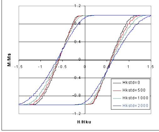
Figure 1: The effect of anisotropy distributions on hysteresis in perpendicular media. A Gaussian distribution of anisotropy fields is used with a mean value of $H_{ku}$ = 7000 Oe. In the bottom left corner, the curves correspond to standard deviations in $H_{K}$ of (from left to right) 2000 Oe, 1000 Oe, 500 Oe, and 0 Oe. The saturation magnetization is 350 emu/cm³. Data courtesy of M. Plumer PLUMER

II.2 Micromagnetics

For systems in which the spins are not aligned and/or the field is changing too rapidly for the magnetization to reach its quasi-static value, it is usually necessary to use a non-perturbative technique such as micromagnetics to describe the reversal process. The basic approach is to divide the system into a coarse-grained set of sites. Each site is associated with a position $\vec{r}_{i}$, and its magnetization is represented by a single magnetization vector $\vec{M}\left(\vec{r}_{i}\right)$, whose norm is the saturation magnetization $M_{S}$, corresponding to the bulk material (a valid assumption for temperatures well below the Curie temperature garanin ). The time evolution of each spin is given by the Landau–Lifshitz–Gilbert (LLG) equation brown ; nowak ; greg1 ,

$$\frac{\mathrm{d}{\vec{M}(\vec{r}_{i})}}{\mathrm{d}t}=\gamma_{0}\left(\vec{M}(\vec{r}_{i})\times\left[\vec{H}(\vec{r}_{i})-\frac{\alpha}{\gamma_{0}M_{S}}\left(\frac{\mathrm{d}\vec{M}(\vec{r}_{i})}{\mathrm{d}t}\right)\right]\right)\;,$$ (3)

where $\vec{H}\left(\vec{r}_{i}\right)$ is the total local field at the $i$-th site, $\gamma_{0}$ is the gyromagnetic ratio $(1.76\times 10^{7}$ rad/Oe s), and $\alpha$ is a dimensionless damping parameter which determines the rate of energy dissipation in the system. The first term represents the precession of each spin around the local field, while the second term drives the magnetization to align with the field. The LLG equation can easily be rewritten in a form more convenient for numerical integration brown ; aharoni

$$\frac{\mathrm{d}\vec{M}(\vec{r}_{i})}{\mathrm{d}t}=\frac{\gamma_{0}}{1+\alpha^{2}}\\ \left(\vec{M}(\vec{r}_{i})\times\left[\vec{H}(\vec{r}_{i})-\frac{\alpha}{M_{S}}\left(\vec{M}(\vec{r}_{i})\times\vec{H}(\vec{r}_{i})\right)\right]\right)\;.$$ (4)

For the sign of the undamped precession term, we follow the convention of Brown brown .

The total local field, $\vec{H}\left(\vec{r}_{i}\right)$, controls the dynamics and contains all of the interactions between each site and the rest of the system; it is defined by

$$\vec{H}\left(\vec{r}_{i}\right)=-\frac{\partial E_{i}}{\partial\vec{M}\left(\vec{r}_{i}\right)}\;.$$ (5)

Here, $E_{i}$ is the free energy of the $i$-th site and the operator $\partial/\partial\vec{M}\left(\vec{r}_{i}\right)=$ $\left(\partial/\partial M_{x}\left(\vec{r}_{i}\right)\right)\hat{x}+\left(\partial/\partial M_{y}\left(\vec{r}_{i}\right)\right)\hat{y}+\left(\partial/\partial M_{z}\left(\vec{r}_{i}\right)\right)\hat{z}$. The different terms that contribute to $\vec{H}\left(\vec{r}_{i}\right)$ combine via linear superposition,

$$\vec{H}(\vec{r}_{i})=\vec{H}_{Z}(\vec{r}_{i})+\vec{H}_{e}(\vec{r}_{i})+\vec{H}_{D}(\vec{r}_{i})+\vec{H}_{a}(\vec{r}_{i})+\vec{H}_{n}(\vec{r}_{i})\;.$$ (6)

Here, $\vec{H}_{Z}\left(\vec{r}_{i}\right)$ is the externally applied field (Zeeman term), $\vec{H}_{e}\left(\vec{r}_{i}\right)$ is due to exchange interactions, $\vec{H}_{D}\left(\vec{r}_{i}\right)$ is the dipole field, $\vec{H}_{a}\left(\vec{r}_{i}\right)$ is the anisotropy field (in our simulations taken to be zero), and $\vec{H}_{n}\left(\vec{r}_{i}\right)$ is a random field representing the effects of thermal noise.

The exchange contribution to the local field represents local variations between the alignment of $\vec{M}\left(\vec{r}_{i}\right)$ and neighboring sites and can be represented by $l_{e}^{2}\nabla^{2}\vec{M}\left(\vec{r}_{i}\right)$ aharoni . In our simulations, this is implemented by

$$\vec{H}_{e}(\vec{r}_{i})=\left(\frac{l_{e}}{\Delta r}\right)^{2}\left(-n_{i}\vec{M}(\vec{r}_{i})+\sum_{\left|d\right|=\Delta r}\vec{M}(\vec{r}_{i}+\vec{d})\right)\;,$$ (7)

where the summation is over the nearest neighbors of $\vec{r}_{i}$, $n_{i}$ is the number of neighbors of site $i$, and the term $n_{i}\vec{M}\left(\vec{r}_{i}\right)$ is included so that $\vec{H}_{e}=0$ when all of the spins are aligned. The exchange length, $l_{e}$, is defined in terms of the exchange energy arrot , $E_{e}=-\left(l_{e}^{2}/2\right)\int d\vec{rM}\cdot\nabla^{2}\vec{M}$, in a continuous system. For our discrete system of finite-sized cells, this means the magnetization can be viewed as rotating continuously from the center of one cell to the center of each neighboring cell along the line joining the two.

At non-zero temperatures, thermal fluctuations contribute a term to the local field in the form of a stochastic field $\vec{H}_{n}\left(\vec{r}_{i}\right)$, which is assumed to fluctuate independently for each spin. The fluctuations are assumed to be Gaussian, with zero mean and (co)variance given by the fluctuation-dissipation theorem brown ; greg1 ,

$$\left\langle H_{n\mu}(\vec{r}_{i},t)H_{n\mu^{\prime}}(\vec{r}_{i}^{\prime},t^{\prime})\right\rangle=\frac{2\alpha k_{B}T}{\gamma_{0}M_{S}V}\delta(t-t^{\prime})\delta_{\mu,\mu^{\prime}}\delta_{i,i^{\prime}}\;,$$ (8)

where $H_{n\mu}\left(\vec{r}_{i}\right)$ indicates one of the Cartesian coordinates of $\vec{H}_{n}\left(\vec{r}_{i}\right)$. Here, $T$ is the absolute temperature, $k_{B}$ is Boltzmann’s constant, $V=\left(\Delta r\right)^{3}$ is the discretization volume of the numerical integration, and $\delta_{r,r^{\prime}}$ is the Kronecker delta representing the orthogonality of the Cartesian components. Although this result was derived for an isolated particle, recent work by Chubykalo, et al. indicates that this result will hold for interacting systems as well CHUBYKALO . In this paper, we present micromagnetic results for two different models. The first model is of a nanoparticle with dimensions 5.2 nm$\times$5.2 nm$\times$88.4 nm. The cross-sectional dimensions are small enough ($\approx$ 2 $l_{e}$) that the assumption is made that the only significant inhomogeneities occur along the long axis ($z$-direction) nowak ; boerner2 . The particles of this model are therefore discretized into a linear chain of 17 spins along the long axis of the particle. We will call this model the stack-of-spins model.

In this simple model, the local field due to dipole-dipole interactions is calculated as arrot ; boerner2

$$\vec{H}_{D}(\vec{r}_{i})=(\Delta r)^{3}\sum_{j\neq i}\frac{3\hat{\vec{r}}_{ij}(\hat{\vec{r}}_{ij}\cdot\vec{M}(\vec{r}_{j}))-\vec{M}(\vec{r}_{j})}{\vec{r}_{ij}^{3}}\;,$$ (9)

where $\vec{r}_{ij}$ is the displacement vector from the center of cube $i$ to the center of cube $j$, and $\hat{\vec{r}}_{ij}$ is the corresponding unit vector. The volume factor $(\Delta r)^{3}$ results from integration over the constant magnetization density in each cell. The second model, which we will refer to as the full micromagnetic model, simulates a single nanoparticle with dimensions 9 nm $\times$ 9 nm $\times$ 150 nm. The dimensions were chosen to correspond to arrays of nanoparticles fabricated by Wirth, et al. wirth1 . In this model, the system is discretized into 4949 sites (7 $\times$ 7 $\times$ 101) on the computational lattice. The size of the system makes calculation of dipole interactions in the conventional manner (as done for the stack-of-spins model) computationally impractical. It is therefore necessary to use a more advanced algorithm to make the simulation tractable.

The two most popular choices are the traditional Fast Fourier Transform (FFT) and the Fast Multipole Method (FMM) greengard . Here, we used the Fast Multipole Method, the exact implementation of which is discussed elsewhere greg1 , because it has several advantages over the FFT. The biggest difference is that the FMM makes no assumptions about the shape of the underlying lattice, while the FFT assumes a cubic lattice with periodic boundary conditions. The consequence of this is that numerical models of systems without periodic boundary conditions which use the FFT require empty space around the system so that the boundary conditions do not affect the calculation. The FMM requires no such “padding”. Furthermore, the FFT requires $O\left(N{\rm ln}N\right)$ operations to calculate the magnetic scalar potential (from which the dipole field is calculated). The FMM algorithm, while it has a larger computational overhead, requires only $O\left(N\right)$ operations for the same calculation. This means that, while the FFT is a good choice for small cubic lattices, the FMM is better for large, incomplete, or irregular lattices. The public-domain psi-Mag toolset now provides a flexible implementation of the FMM designed for use on high performance, parallel computers greg2 .

Material properties in both models were chosen to correspond to bulk Fe. The saturation magnetization is 1700 emu/cm³ (kA/m) and $l_{e}=2.6$ nm. We take the damping parameter $\alpha=0.1$ to correspond to the underdamped behavior usually assumed to be present in nanoscale magnets. Although this value is approximately an order of magnitude larger than the value obtained experimentally using Ferromagnetic Resonance (FMR), it has been noted that the FMR value is for small deviations of the magnetization from equilibrium and is not representative of the large deviations which occur during reversal stinnett1 . In general, care should be taken in establishing an appropriate damping parameter to use in simulating a particular magnetic nanostructure, as also illustrated in other recent micromagnetic studies fidler ; hertel ; boerner1 .

It is worth noting that, even in systems which reverse coherently at high speed, deviations from the quasi-static Stoner–Wohlfarth (SW) model will be expected. He, et al. He showed that for square-pulse fields with fast rise times ($<$ 10 ns) and small values of the damping constant ($<$ 0.2), the shape of the astroid changes. The result is that the minimum switching field is reduced below the SW limit of 0.5 $H_{K}$, and the angular dependence is no longer symmetric around 45^∘. For the frequencies and damping parameter used here, the deviations from the SW model are small ($<$ 5 percent difference in the switching fields) and may be neglected.

II.3 Monte Carlo Simulations: Kinetic Ising and Heisenberg Models

A second approach to modeling the dynamics of magnetic systems involves Monte Carlo techniques, which have been applied to a wide variety of systems since their introduction by Metropolis, et al. metropolis . As described above, the micromagnetics approach uses a stochastic (i.e. random number-based) variable to introduce random fluctuations into an otherwise deterministic system. In contrast, Monte Carlo simulations are fully stochastic and proceed by considering possible transitions between states of the system and executing these transitions with a probability which depends on the system’s energy and temperature.

The static Monte Carlo algorithm consists of a repeated three-step process. First, choose a (pseudo-)random number. The random numbers chosen may be uniformly distributed, or they may be chosen based on a particular probability distribution that depends on the specific simulation to be performed. Second, choose a trial move from the current state to a new state. Third, accept or reject the trial move depending on the random number and some acceptance rule consistent with the problem under consideration.

Consider the ferromagnetic Ising model on a regular lattice with periodic boundary conditions. Each site on the lattice has a spin which can align either parallel or anti-parallel to the applied field and takes on values of $S_{i}=\pm 1$ accordingly. The energy of the Ising lattice is then

$$E=-J\sum_{\langle i,j\rangle}S_{i}S_{j}-H(t)\sum_{i}S_{i}\;,$$ (10)

where the exchange constant $J>0$ is in units of energy, and $H(t)$ is the externally applied, time-dependent magnetic field (which in Monte Carlo simulations is customarily given in units of energy, thus absorbing the magnetic moment per site, $\mu$). The first sum in (10) is over nearest-neighbor pairs, while the second sum is over all spins on the lattice.

The static Monte Carlo procedure described above allows the calculation of equilibrium quantities such as the internal energy, susceptibility, specific heat, and magnetization. In order for the lattice to explore each of its possible states with probabilities corresponding to the equilibrium thermal distribution, the acceptance rule chosen must satisfy the condition of detailed balance Landau . Two common choices are the Metropolis metropolis and Glauber GLAUBER acceptance rules. Note that near the critical point, computation with these simple acceptance rules slows down dramatically, and it is therefore useful to use more advanced algorithms (such as cluster algorithms Landau ) to calculate equilibrium quantities.

In equilibrium calculations, no physical interpretation is ascribed to the intermediate spin flips. If, instead, we consider the individual spin flips as representing physical fluctuations due to the interactions between the spins and a heat bath, then the underlying transitions model the actual dynamics of the system and acquire a physical significance. This application of Monte Carlo simulations is known as kinetic Monte Carlo. The random nature of the events due to the interaction of spins dictates that the spin to attempt to flip must be chosen at random. In this paper, we use the Glauber GLAUBER acceptance rule, according to which each attempted spin flip is accepted with probability

$$W~{}=~{}\frac{\exp\left(-\beta\Delta E_{i}\right)}{1+\exp\left(-\beta\Delta E_{i}\right)}\;.$$ (11)

Here, $\Delta E_{i}$ is the change in energy that results if the proposed flip of the $i$-th spin is accepted, and $\beta$ = $\left(k_{B}T\right)^{-1}$. With a uniformly distributed random number, $r\in[0,1]$, a randomly chosen spin is flipped if $r~{}\leq W$. Each potential spin flip is considered a Monte Carlo step. The basic time step of the Monte Carlo process is measured in Monte Carlo Steps per Site (MCSS). This time is related to the algorithm and in general is only approximately proportional to the physical time of the system. Recently, however, progress has been made in connecting analytically the MC simulation time to the simulation time of the Langevin-based micromagnetic techniques discussed above, for which there is a clear relationship to physical time  nowak2 ; chubykalo2 ; cheng1 ; cheng2 .

The Glauber dynamic of (11) can be derived from a quantum spin-$\frac{1}{2}$ Hamiltonian coupled to a fermionic heat bath MARTIN . Recently, other dynamics have been derived from coupling a quantum spin-$\frac{1}{2}$ system to a phonon heat bath PARK . Note that in kinetic Monte Carlo calculations, algorithms (such as the cluster algorithm) that change the underlying dynamic cannot be used. However, advanced algorithms that achieve very large speedups while remaining true to the underlying dynamics are possible novotny . It has recently been shown that physically relevant functional forms for $W$ can lead to dramatically different values of dynamical quantities such as lifetimes of metastable states NEWPRL .

It is important to realize that the Monte Carlo techniques can be applied to other systems as well. Unlike the Ising model, the Heisenberg model allows the spins to assume any angle with respect to neighboring spins and the applied field. The energy of a regular lattice of Heisenberg spins with periodic boundary conditions is

$$E=-J\sum_{\langle i,j\rangle}(S_{ix}S_{jx}+S_{iy}S_{jy}+S_{iz}S_{jz})-H\sum_{i}S_{i}\cos(\theta_{i})\;,$$ (12)

where $S_{ix}$, $S_{iy}$, and $S_{iz}$ are the Cartesian coordinates of the vector spin $\textbf{S}_{i}$ (with magnitude $S_{i}=1$), and $\theta_{i}$ is the angle between the applied field, $H$, and the $i$-th spin. As in the Ising model, the first sum is taken over nearest neighbors and represents the exchange interactions, while the second sum is taken over all spins in the system, and represents the interactions of the spins with an externally applied magnetic field (Zeeman energy).

The dynamic consists of randomly choosing a spin to update, randomly choosing a new spin direction (either uniformly distributed over the sphere or over a cone near the current spin direction), and using a Metropolis or a heat-bath rate to decide whether to effect a transition to the new spin direction. The rate depends on the energy difference between the spin configurations as in, for example, (11).

In kinetic Monte Carlo, it is possible to implement the algorithm in a rejection-free manner, so that every algorithmic step performs an update. In this case, each algorithmic step in general advances the system by a different amount of time. For models, such as the Ising model, with discrete state spaces this is called the $n$-fold way algorithm bortz . It is possible to make a precise connection between these the $n$-fold way and the standard implementation of kinetic Monte Carlo novotny . Recently such rejection-free methods have been implemented for models with continuous state spaces, such as the Heisenberg model MUNOZ , and the efficiency of rejection-free methods in various systems has been studied watanabe .

III Results of Micromagnetic Simulations

In this section we summarize recent simulation results for magnetization reversal in iron nanopillars greg4 , and further evaluate these results in light of additional experimental data on such reversal.

Figure 2a shows hysteresis loops at $T$ $=$ 100 K for the full micromagnetic model with the field misaligned at $0^{\circ}$, $45^{\circ}$, and $90^{\circ}$ to the long axis of the particle. The loops were calculated using a sinusoidal field with a period of 25 ns, which started at a maximum value of 10,000 Oe (800 kA/m). In all the loops in this section, the reported magnetization is the component along the long axis ($z$-axis) of the particle. Simulations for the full micromagnetic model were performed over one half of the period and the results reflected to give the full hysteresis loop.

Consider the case with the field and particle aligned ($0^{\circ}$). Initially, the large magnetic field tends to align the spins with the easy axis. As the field is decreased, the spins relax, and the magnetization decreases by approximately $2\%$. Eventually, reversal initiates at the ends as previously reported greg1 .

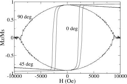
(a) Hysteresis loops for the full micromagnetic model at $T$ $=$ 100 K with a sinusoidal field of period 25 ns and maximum applied field of 10 kOe

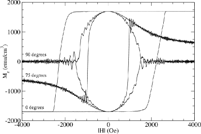
(b) Hysteresis loops for the stack-of-spins model at $T$ $=$ 10 K with a sinusoidal field of period 200 ns and a maximum applied field of 5 kOe

Figure 2: Hysteresis loops for (a) the full micromagnetic model with 0^∘, 45^∘, and 90^∘ misalignment and (b) the stack-of-spins model with 0^∘, 75^∘, and 90^∘ between the applied field and the long axis of the particle

At $45^{\circ}$ misalignment between the particle and the field, the magnetization is initially pulled away from the long (easy) axis by the large magnetic field. As the field is swept toward zero, the magnetization relaxes until it essentially reaches a maximum value of approximately $0.91M_{S}$ at zero applied field. Thermal fluctuations along the length of the particle prevent the magnetization from reaching saturation. As in the case of 0^∘, reversal again begins by nucleation at the ends of the particle, with the growth of these nucleated regions leading to the reversal of the particle. Figure 3a shows the $z$-component of the magnetization at selected times during the reversal process for the $45^{\circ}$ hysteresis loop of Fig. 2a. It is important to note that the particles do not have a uniform magnetization during the reversal process, even though they are single-domain particles.

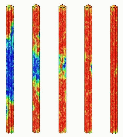
(a) Snapshots of reversal at times (left to right) $t$ $=$ $7.350$, $7.375$, $7.400$, $7.425$, and $7.450$ ns

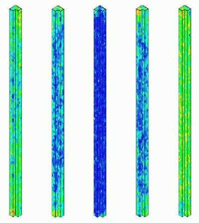
(b) Snapshots of reversal at times (left to right) $t$ $=$ $0.00$, $3.000$, $4.000$, $6.250$, and $8.500$ ns

Figure 3: The $z$-component of the magnetization in the full micromagnetic model for the (a) 45^∘ and (b) 90^∘ hysteresis loops of Fig. 1a

For $90^{\circ}$ misalignment, the reversal mechanism is quite different. The hysteresis loop in Fig. 2a shows that the magnetization is essentially perpendicular to the easy direction until the field reaches a particular value. As the field is decreased further, the magnetization relaxes toward the easy axis. Since nothing breaks the up/down symmetry of the system when the applied field has no component along the easy axis, the relaxed magnetization can be directed toward either the positive or negative $z$-axis. Figure 3b shows the $z$-component of the magnetization for the $90^{\circ}$ misalignment at selected times during the hysteresis loop of the full micromagnetic model. For this case, the nucleation occurs along the entire length of the particle, except at the ends. The large demagnetizing fields present at the ends (involved in nucleation at smaller angles) retard relaxation along the easy axis.

The hysteresis loops for the stack-of-spins model, shown in Fig. 2b, are qualitatively similar to those of Fig. 2a. Loops at $0^{\circ}$, $75^{\circ}$, and $90^{\circ}$ misalignment are shown. There are important differences between the two models, however. First, without lateral resolution of the magnetization across the cross-section, these particles exhibit ringing due to the precessional dynamics. Evidently, the precession of individual moments in the full micromagnetic model does not lead to precession of the end-cap moment; possibly the spin waves rapidly damp out the gyromagnetic motion.

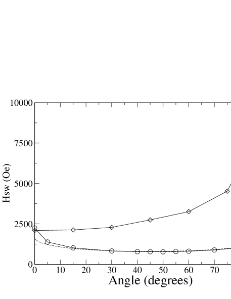
Figure 4: Angular dependence of the switching field for three models of magnetization reversal. The full micromagnetic model (diamonds) at $T$ $=$ 100 K shows a distinctly different behavior from both the stack-of-spins model at $T$ $=$ 20 K (circles) and the Stoner–Wohlfarth model (dashed line)

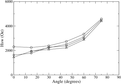
(a) Applied field periods are 15 ns (circles), 25 ns (squares), 50 ns (diamonds), and 100 ns (triangles). The field is sinusoidal with a maximum value of 5 kOe

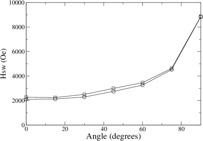
(b) Applied field periods are 15 ns (squares) and 25 ns (circles). The field is sinusoidal with a maximum value of 10 kOe

Figure 5: Angular dependence of the switching field for the full micromagnetic model at (a) 0 K and (b) 100 K. At 0 K, the LLG equation is completely deterministic, while at 100 K, it includes random fluctuations through a stochastic thermal field.

A second, and more prominent, difference between the models is observed in the angular dependence of the switching field, $H_{{\rm sw}}$, shown in Fig. 4. Here, $H_{{\rm sw}}$ is defined as the applied field at which $M_{z}$ is reduced to 0. The stack-of-spins model (circles) shows a shape qualitatively similar to what is expected from Stoner–Wohlfarth (SW) theory, with a minimum $H_{{\rm sw}}$ near $45^{\circ}.$ The dashed curve is the SW theory with $H_{K}$ $=$ 1600 Oe (for comparison reasons $H_{K}$ was chosen to be much smaller than the $10^{4}$ Oe expected for these particles assuming SW behavior). The full micromagnetic model (diamonds), on the other hand, has its minimum $H_{{\rm sw}}$ at $0^{\circ},$ and $H_{{\rm sw}}$ increases as the misalignment angle is increased. Figure 5 shows the angular dependence of the switching field for the full micromagnetic model for periods of 15, 25, 50, and 100 ns and maximum applied field of 5 kOe at $T$ $=$ 0 K, and for periods of 15 ns and 25 ns with a maximum applied field of 10 kOe at $T$ $=$ 100 K. At 0 K, the general trend is for longer periods to reduce the switching field. However, at $15^{\circ}$, the 100 ns loop is observed to switch at a lower field than either the 50 or 25 ns loops. Similarly, at $30^{\circ}$, the 50 ns loop switches at a lower field than the 25 ns loop. One reason for this may be resonance in the switching fields for these angles and periods. At $T$ $=$ 100 K, the 25 ns loops switch at a lower field than the 15 ns loops for all angles. At $90^{\circ}$, where thermal fluctuations are most prominent, the field at which relaxation occurs is independent of the period within the accuracy of the simulation.

The increase of $H_{\rm{sw}}$ with the misalignment angle in the micromagnetic simulation is consistent with recent experimental observations of Fe nanopillars wirth1 ; wirth2 ; Li1 ; Li2 ; Li3 . However, the most recent experiment Li3 shows that a nanopillar with lateral dimension $d\sim 5.2~{}\mathrm{nm}$, which our formulation suggests should show a dependence of $H_{\rm{sw}}$ on misalignment angle similiar to the stack-of-spins model (i.e. like coherent rotation), actually exhibits the increasing dependence found in the full micromagnetic model. In addition, a nanopillar with lateral dimension $d\sim 10-15~{}\mathrm{nm}$ showed evidence of a multi-domain remanence state. As noted in Ref. Li3, , imperfections of the nanopillar structure appear to contribute to localized nucleation processes down to smaller than expected lateral dimensions, and probably also provide the pinning sites causing the multi-domain remanence state. This illustrates the importance of coordinating experimental and simulation results in the micromagnetic approach. Further improvement of the predictions of the micromagnetic approach will likely have to incorporate such structural imperfections.

IV Recent Results for the 2D Kinetic Ising Model

Monte Carlo simulation of the Ising model, as well as other magnetic systems, continues to be an active field of research. Here, we present three recent results that are of interest in understanding the process of magnetization reversal in ultra-thin films.

IV.1 Dynamic Phase Transitions

When the half-period $t_{1/2}$ of the applied field is longer than the characteristic switching time in a constant field, $\langle\tau(H_{0})\rangle$, where $H_{0}$ is the amplitude of the oscillating field, the magnetization can follow the changing field, resulting in standard hysteresis loops, such as those shown in Fig. 1 and in Fig. 6a. However, when $t_{1/2}\ll\langle\tau(H_{0})\rangle$, the magnetization cannot follow the field, but rather oscillates around one or the other of its zero-field stable values. This breaking of the symmetry of the hysteresis loop is associated with a dynamic phase transition (DPT) located at an intermediate value of the half-period. In terms of the dimensionless half-period, $\varTheta=t_{1/2}/\langle\tau(H_{0})\rangle$, the transition is located at $\Theta_{c}\approx 1$. The dynamic order parameter for this transition is the period-averaged magnetization,

$$Q_{n}=\frac{1}{2t_{1/2}}\int_{(n-1)(2t_{1/2})}^{n(2t_{1/2})}{m(t)\mathrm{d}t}\;.$$ (13)

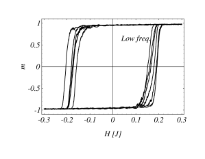
Figure 6: Simulated hysteresis loops for a kinetic Ising model (a) in the dynamically disordered phase for $\varTheta\gg\varTheta_{c}$ and (b) in the dynamically ordered phase for $\varTheta\ll\varTheta_{c}$. Data courtesy of S.W. Sides

In Fig. 6, we show hysteresis loops for the two-dimensional kinetic Ising model using Glauber dynamics for the dynamically disordered phase with $\varTheta\gg\varTheta_{c}$ and the dynamically ordered phase with $\varTheta\ll\varTheta_{c}$. Time series of $Q_{n}$ for $\varTheta\gg\varTheta_{c}$, $\varTheta\approx\varTheta_{c}$, and $\varTheta\ll\varTheta_{c}$ are shown in Fig. 7.

Figure 7: Time series of the dynamic order parameter $Q_{n}$ in the dynamically ordered phase (curve near +1, $\varTheta$ $=$ 0.27), near the transition (curve fluctuating wildly about zero, $\varTheta$ $=$ 0.98), and in the dynamically disordered phase (curve that remains close to zero, $\varTheta$ = 2.7). After  ISING3

The DPT was first discovered in numerical solutions of a mean-field model of a ferromagnet in an oscillating field TOME ; MENDES . It has since been intensively studied in mean-field models MFA1 ; MFA2 ; MFA3 , kinetic Ising models  ISING1A ; ISING1B ; ISING1C ; ISING2 ; ISING3 ; ISING4 , the kinetic spherical model  Paessens , and anisotropic $XY$  TUTU ; fujiwara and Heisenberg JANG ; huang models. There have also been indications of its presence in experimental studies of hysteresis in ultra-thin films of Cu on Co(001) EXP ; EXP2 . From a theoretical point of view, its most interesting feature is that this far-from-equilibrium phase transition is a genuine continuous (second-order) phase transition that belongs to the same universality class as the equilibrium phase transition in the Ising model in zero field ISING2 ; ISING3 ; ISING4 ; FUJI . Unequivocal experimental verification of this interesting non-equilibrium phase transition is highly desirable and, given that new high-density magnetic recording media will require shorter reversal periods, may be relevant to the design of magnetic storage devices.

IV.2 Hysteresis Loop Area and Stochastic Resonance

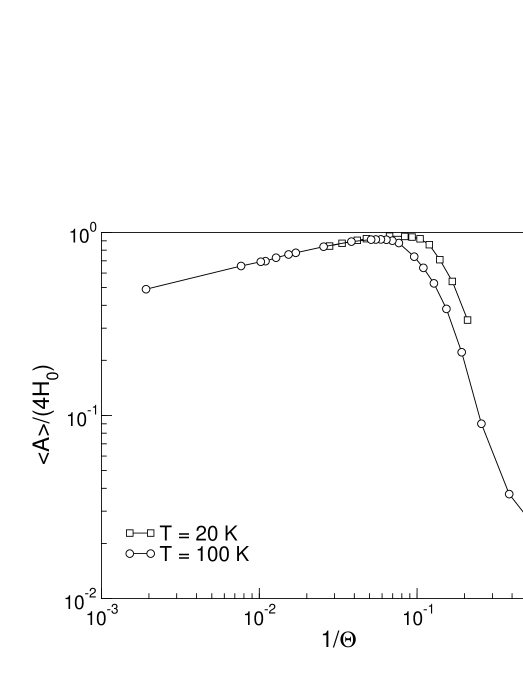
Figure 8: Average hysteresis-loop area, $\langle A\rangle$, vs scaled frequency, $1/\varTheta$ for the stack-of-spins micromagnetic model. The same behavior is seen in two-dimensional Ising models that switch by a single-droplet mechanism, and the maximum is associated with stochastic energy resonance

The values of $Q$ measured for the stack-of-spins model described above appear to be consistent with the existence of a DPT, although no detailed analysis has yet been made greg3 . At lower frequencies, another interesting behavior is seen in both the stack-of-spins and kinetic Ising models greg3 ; SIDES . The normalized average hysteresis-loop area,

$$\langle A\rangle=-\frac{1}{4M_{S}H_{0}}\oint M\left(H\right)\mathrm{d}H\;,$$ (14)

is a measure of the average energy dissipation per period and is therefore a very important quantity. It is shown vs scaled frequency, $1/\varTheta$, in Fig. 8 for the stack-of-spins model at $T$ $=$ $100$ K and $T$ $=$ $20$ K. At extremely low frequencies, the magnetization switches at very small values of $H$, so that $\langle A$$\rangle$ $\approx$ $0$. At high frequencies, the switching rarely completes because the system is metastable for only a very short time interval. Therefore, $M$ is nearly constant and again $\langle A\rangle$ $\approx$ $0$. A maximum in $\langle A\rangle$ occurs at intermediate frequencies $1/\varTheta$ $\approx$ $0.1$. For studies of hysteresis in a kinetic Ising model which switches by a single-droplet mechanism, this maximum was found to correspond to stochastic energy resonance SIDES . This phenomenon has been studied further in the kinetic Ising model ISING4 ; acharyya ; kim , and also recently investigated in models of superparamagnetic nanoparticles raikher and Preisach systems mantegna .

IV.3 First-Order Reversal Curves

The First-Order Reversal Curve (FORC) technique was developed by Pike, et al. PIKE1 in order to extract more information from magnetic samples than is represented by, for example, the coercive field or the remanent magnetization. The FORC method has since been applied to a wide variety of systems, including several relevant to magnetic nanostructures PIKE3 ; carvallo ; bercoff ; oliva ; spinu ; davies ; PIKE4 ; davies2 . In addition, progress has been made in understanding the role of reversible magnetization in the FORC method PIKE5 and in improving the efficiency of its computational use heslop . Here, we illustrate the basic approach with an application to the kinetic Ising model.

The FORC technique involves decreasing the applied field from a positive saturating field, $H_{0}$, to a series of progressively more negative return fields, $H_{r}$, and recording the normalized magnetization, $m$$=$$M/M_{S}$, as the field is increased from each of these return fields back to the positive saturating field. This process results in a family of first-order reversal curves, $m(H_{r},H)$, where $H$ represents the applied magnetic field as it is increased from $H_{r}$ back to $H_{0}$. Since the first-order reversal curves (FORCs) are determined by the type of reversal that has taken place before reaching $H_{r}$, the full family of FORCs should contain useful information about the mechanisms of reversal.

We can use the FORC method to better understand the process of hysteresis in the two-dimensional ferromagnetic kinetic Ising model on a square lattice, choosing the Glauber acceptance rule to produce the dynamic of the system with the energy given by (10). While most FORC studies have been done on systems with strong disorder, we focus here on the square-lattice Ising model without disorder. Our simulations were performed at a temperature of $T=0.8~{}T_{c}$ which, given that $k_{B}T_{c}\approx 2.269J$ for the two-dimensional square-lattice Ising model, corresponds to $k_{B}T\approx 1.815J$. It has been found RIKVOLD1 that the switching of a fully magnetized lattice for these parameters occurs through single-droplet nucleation for fields up to $|H|\approx 0.35$, by multi-droplet nucleation for fields $|H|\approx$ 0.35–0.9, and by strong-field (single-spin) reversal for fields $|H|>0.9$. Since the process of switching is also influenced by the lattice size for finite lattices, these values serve only as guidelines. Here, we are mainly concerned with the multi-droplet regime, and so choose $H_{0}=0.55$.

We performed MC simulations to calculate the characteristic switching time $\tau$ (for switching from $m=1.0$ to $m<-0.8$) in a field of magnitude $H_{0}=-0.55$, finding $\tau\approx 100$ MCSS for a 128 $\times$ 128 lattice. We therefore chose a field period of $P=1000$ MCSS, corresponding to a dimensionless half-period $\varTheta~{}=\frac{P/2}{\tau}\approx 5$. The form of the field is taken as a sawtooth, piecewise linear function

$${H}(t)={H}_{0}\left(\frac{4|t-P/2|}{P}-1\right)\;.$$ (15)

Figure 9a shows the results of the simulation on a 128 $\times$ 128 lattice for dimensionless half-periods of $\varTheta~{}=~{}5$, $10$, and $25$. The simulations were performed in parallel with 100 independent realizations distributed over 20 processors using the 48-bit linear congruential random number generator included with the SPRNG 2.0 package SPRNG .

 

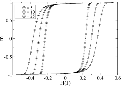
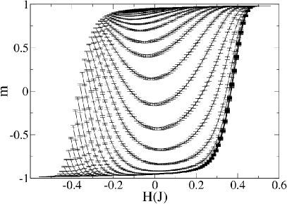
Figure 9: (a)Hysteresis loops for $\varTheta$=5 (solid line), 10 (dashed line), and 25 (dotted line) on a 128 $\times$ 128 Ising lattice. (b) Family of FORCs for the same lattice with $\varTheta$ = 5

As the lattice just completes its reversal during the full hysteresis loop, we expect that the family of FORCs will reflect much of the dynamics that are occurring during the reversal. To investigate this, we divided the interval from $H=[-0.55,0.55]$ into 100 equal intervals. We began the first FORC at a return field of $H_{r}=0.0$, and recorded the magnetization at $H_{a}$ values corresponding to the endpoints of the 100 intervals. (Thus, for the first FORC, we took 51 values of the magnetization.) We then took a series of FORCs for $H_{r}$ values at the interval endpoints from $H=0.0$ to $H=-0.55$, producing a total of 51 FORCs. For each curve, we averaged over 100 realizations of the MC simulation, a technique commonly used to find the thermally averaged behavior of a system. The resulting family of FORCs is shown in Fig. 9b. An animation of the reversal process for the FORCs shows that the reversal does proceed by the nucleation, growth, and shrinkage of multiple droplets (i.e., areas of reversed magnetization).

In a recent article robb , we have continued this investigation of the kinetic Ising model using the family of FORCs, as well as the FORC distribution, which can be derived from the FORCs as described in Ref. PIKE1, . The analysis yielded insights into the limits of application of the Kolmogorov-Johnson-Mehl-Avrami (KJMA) model of phase transformation kjma1 ; kjma2 ; kjma3 to the kinetic Ising system. In general, the FORC method appears to be quite sensitive to details of the magnetization reversal process, and with some thought can be helpful in developing insights into the construction of useful models.

V Conclusion

Information storage devices utilizing magnetic nanostructures have become a technologically important part of our society. As demands for information storage increase, the size of the nanostructures must be decreased. At the same time, it becomes important to read and write the information to these devices (i.e. reverse the magnetization) faster. The understanding of hysteresis in the magnetic nanostructures is therefore important to the continued growth of the information-storage industry. At the same time, the growth of computational resources has provided researchers with an invaluable tool with which to better understand these systems.

In this overview, various common models and methods for simulating hysteresis in magnetic nanostructures have been presented along with results illustrating some of the properties of these systems. Micromagnetic simulations are accomplished by integration of the Landau-Lifshitz-Gilbert (LLG) equation. The LLG equation, despite being both classical and phenomenological in origin, nevertheless provides good insight into the magnetization dynamics at nanosecond time scales, provided the system is sufficiently finely discretized. Our simulations on single Fe nanopillars show that the switching field (i.e. the field required to reduce $M_{Z}$ to 0) increases continuously as the angle between the $z$-axis and the applied field direction is increased, consistent with experiment. Reversal in these pillars is shown to nucleate at the endcaps and proceed by domain growth towards the center of the particle. The exception to this is the case of the applied field perpendicular to the long axis of the pillar, in which nucleation of reversal occurs along the whole length of the particle.

Unfortunately, limitations on computer resources prevent extension of micromagnetic simulations beyond timescales of a few tens of nanoseconds. For timescales where the transition time for an individual spin to relax from the metastable to the stable state is much shorter than the time scale of interest, individual spin reversals occur with a probability which is related to the Boltzmann factor. The dynamics of the system can then be modeled using kinetic Monte Carlo techniques with either the Ising or Heisenberg models. Here, we have shown three interesting applications of kinetic Monte Carlo simulations of a 2-D Ising model to understanding hysteresis: dynamic phase transitions, stochastic resonance in the hysteresis loop area, and First-Order Reversal Curves (FORCs). These illustrate only a few of the ways simulations of magnetic nanostructures may help give new insight into this important class of materials for ultra-high-density data storage.

References

- (1) http://en.wikipedia.org/wiki/Serial_ATA
- (2) eWeek, Jan. 17, 2006 (formerly PC Week magazine, now online only at http://www.eweek.com)
- (3) M. Plumer, J. van Ek: Micromagnetic System Modeling for Perpendicular Recording, presented at the Micromagnetics and Magnetic Recording Workshop held at the Center for Materials for Information Technology, the University of Alabama (November 6, 2003) (unpublished)
- (4) K.Z. Gao, H.N. Bertram: IEEE Trans. Magn. 39, 704 (2003)
- (5) K.Z. Gao, J. Fernandez-de-Castro, H.N. Bertram: IEEE Trans. Magn. 41, 4236 (2005)
- (6) O. Perković, K. Dahmen, J.P. Sethna: Phys. Rev. Lett. 75, 4528 (1995)
- (7) K. Dahmen, J.P. Sethna: Phys. Rev. B 53, 14872 (1996)
- (8) J.H. Carpenter, K. Dahmen, J.P. Sethna, G. Friedman, S. Loverde, A. Vanderveld: J. Appl. Phys. 89, 6799 (2001)
- (9) E.C. Stoner, E.P. Wohlfarth: Phil. Trans. Roy. Soc. A240, 599 (1948)
- (10) D.A. Garanin: Phys. Rev. B 55, 3050 (1997)
- (11) W. Brown: Micromagnetics (Wiley, 1963)
- (12) U. Nowak: Thermally Activated Reversal in Magnetic Nanostructures. In: Annual Reviews of Computational Physics IX, ed. by D. Stauffer (World Scientific, Singapore 2001) pp. 105–152
- (13) G. Brown, M.A. Novotny, and P.A. Rikvold: Phys. Rev. B 64, 134432 (2001)
- (14) A. Aharoni: Introduction to the Theory of Ferromagnetism (Clarendon, Oxford 1996)
- (15) A.S. Arrot, B. Heinrich, D.S. Bloomberg: IEEE Trans. Magn. MAG-10, 950 (1974)
- (16) O. Chubykalo, R. Smirnov-Rueda, J.M. Gonzalez, M.A. Wongsam, R.W. Chantrell, U. Nowak: J. Magn. Magn. Mater. 266, 28 (2003)
- (17) E. Boerner, H.N. Bertram: IEEE Trans. Magn. 33, 3052 (1997)
- (18) S. Wirth, M. Field, D.D. Awschalom, S. von Molnár: Phys. Rev. B 57, R14028 (1998)
- (19) L.F. Greengard: The Rapid Evaluation of Potential Fields in Particle Systems (MIT Press, Cambridge 1988)
- (20) G. Brown, T.C. Schulthess, D.M. Apalkov, P.B. Visscher: IEEE Trans. Magn. 40, 2146 (2004)
- (21) W.D. Doyle, S. Stinnett, C. Dawson, L.He: J. Magn. Soc. Jpn. 22, 91 (1998)
- (22) J. Fidler, T. Schrefl, W. Scholz, D. Suess, V.D. Tsiantos, R. Dittrich, M. Kirschner: Physica B 343, 200 (2004)
- (23) R. Hertel, J. Kirschner: J. Magn. Magn. Mater. 270, 364 (2004)
- (24) E.D. Boerner, K.Z. Gao, R.W. Chantrell: IEEE Trans. Magn. 40, 2371 (2004)
- (25) L. He, W.D. Doyle, H. Fujiwara: IEEE Trans. Magn. 30, 4086 (1994)
- (26) N. Metropolis, A.W. Rosenbluth, M.N. Rosenbluth, A.H. Teller, E. Teller: J. Chem. Phys. 21, 1087 (1953)
- (27) D. Landau and K. Binder: A Guide to Monte Carlo Simulations in Statistical Physics (Cambridge University Press, Cambridge 2000)
- (28) R.J. Glauber: J. Math. Phys. 4, 294 (1963)
- (29) U. Nowak, R.W. Chantrell, E.C. Kennedy: Phys. Rev. Lett. 84, 163 (2000)
- (30) O. Chubykalo, U. Nowak, R. Smirnov-Rueda, M.A. Wongsam: Phys. Rev. B 67, 064422 (2003)
- (31) X.Z. Cheng, M.B.A. Jalil, H.K. Lee, Y. Okabe: Phys. Rev. B 72, 094420 (2005)
- (32) X.Z. Cheng, M.B.A. Jalil, H.K. Lee, Y. Okabe: http://www.arxiv.org/cond-mat/0602011 (2006) (to appear in Phys. Rev. Lett.)
- (33) P. A. Martin: J. Stat. Phys. 16, 149 (1977)
- (34) K. Park, M.A. Novotny, P.A. Rikvold: Phys. Rev. E 66, 056101 (2002)
- (35) M.A. Novotny: A Tutorial on Advanced Dynamic Monte Carlo Methods for systems with Discrete State Spaces. In: Annual Reviews of Computational Physics IX, ed. by D. Stauffer (World Scientific, Singapore 2001) pp. 153–210 (also available at http://www.arxiv.org/cond-mat/0109182)
- (36) K. Park, P.A. Rikvold, G.M. Buendía, M.A. Novotny: Phys. Rev. Lett., 92 015701 (2004); G.M. Buendía, P.A. Rikvold, K. Park, M.A. Novotny: J. Chem. Phys. 121, 4193 (2004); G.M. Buendía, P.A. Rikvold, M. Kolesik: Phys. Rev. B 73, in press (2006)
- (37) A.B. Bortz, M.H. Kalos, and J.L. Lebowitz: J. Comput. Phys. 17, 10 (1975)
- (38) J.D. Muñoz, M.A. Novotny, S.J. Mitchell: Phys. Rev. E 67, 026101 (2003)
- (39) H. Watanabe, S. Yukawa, M.A. Novotny, N. Ito: http://www.arxiv.org/cond-mat/0508652 (2005) (submitted to Phys. Rev. Lett.)
- (40) G. Brown, S.M. Stinnett, M.A. Novotny, P.A. Rikvold: J. Appl. Phys. 95, 6666 (2004)
- (41) S. Wirth, S. von Molnár: J. Appl. Phys. 85, 5249 (1999)
- (42) Y. Li, P. Xiong, S. von Molnár, S. Wirth, Y. Ohno, H. Ohno: Appl. Phys. Lett. 80, 4644 (2002)
- (43) Y. Li, P. Xiong, S. von Molnár, Y. Ohno, H. Ohno: J. Appl. Phys. 93, 7912 (2003)
- (44) Y. Li, P. Xiong, S. von Molnár, Y. Ohno, H. Ohno: Phys. Rev. B 71, 214425 (2005)
- (45) T. Tomé, M.J. de Oliveira: Phys. Rev. A 41, 4251(1990)
- (46) J.F.F. Mendes, J.S. Lage: J. Stat. Phys. 64, 653 (1991)
- (47) P. Jung, G. Gray, R. Ray, P. Mandel: Phys. Rev. Lett. 65, 1873 (1991)
- (48) M.F. Zimmer: Phys. Rev. E 47, 3950 (1993)
- (49) E.Z. Meilikhov: JETP Letters 79, 620 (2004)
- (50) W.S. Lo, R.A. Pelcovits: Phys. Rev. A 42, 7471 (1990)
- (51) M. Acharyya, B. Chakrabarti: Phys. Rev. B 52, 6550 (1995)
- (52) M. Acharyya: Phys. Rev. E 56, 2407 (1997)
- (53) S.W. Sides, P.A. Rikvold, M.A. Novotny: Phys. Rev. Lett. 81, 834 (1998); Phys. Rev. E 59, 2710 (1999)
- (54) G. Korniss, C.J. White, P.A. Rikvold, M.A. Novotny: Phys. Rev. E 63, 016120 (2000)
- (55) G. Korniss, P.A. Rikvold, M.A. Novotny: Phys. Rev. E 66, 056127 (2002)
- (56) M. Paessens, M. Henkel: J. Phys. A 36, 8983 (2003)
- (57) T. Yasui, H. Tutu, M. Yamamoto, H. Fujisaka: Phys. Rev. E 66, 036123 (2002); erratum: ibid. 67, 019901(E) (2003)
- (58) N. Fujiwara, H. Tutu, H. Fujisaka: Phys. Rev. E 70, 066132 (2004)
- (59) H. Jang, M.J. Grimson, C.K. Hall: Phys. Rev. B 67, 094411 (2003)
- (60) Z.G. Huang, F.M. Zhang, Z.G. Chen, Y.W. Du: Eur. Phys. J. B 44, 423 (2005)
- (61) Q. Jiang, H.-N. Yang, G.C. Wang: Phys. Rev. B 52, 14911 (1995)
- (62) Q. Jiang, H.-N. Yang, G.C. Wang: J. Appl. Phys. 79, 5122 (1996)
- (63) H. Fujisaka, H. Tutu, P.A. Rikvold: Phys. Rev. E 63, 016109 (2001); erratum: ibid. 63, 059903(E) (2001)
- (64) G. Brown, M.A. Novotny, P.A. Rikvold: Physica B 306, 117 (2001)
- (65) S.W. Sides, P.A. Rikvold, M.A. Novotny: Phys. Rev. E 57, 6512 (1998)
- (66) M. Acharyya: Phys. Rev. E 59, 218 (1999)
- (67) B.J. Kim, P. Minnhagen, H.J. Kim, M.Y. Choi, G.S. Jeon: Europhys. Lett. 56, 333 (2001)
- (68) Y.L. Raikher, V.I. Stepanov, R. Perzynski: Physica B 343, 262 (2004)
- (69) R.N. Mantegna, B. Spagnolo, L. Testa, M. Trapanese: J. Appl. Phys. 97, 10E519 (2005)
- (70) C.R. Pike, A. Roberts, K. Verosub: J. Appl. Phys. 85, 6660 (1999)
- (71) C.R. Pike, A.P. Roberts, M.J. Dekkers, K. Verosub: Phys. Earth Planet. Inter. 126, 11 (2001)
- (72) A. Roberts, C.R. Pike, K. Verosub: J. Geophys. Res. 105, 28461 (2001)
- (73) C.R. Pike, A. Fernandez: J. Appl. Phys. 85, 6668 (1999)
- (74) C. Carvallo, A.R. Muxworthy, D.J. Dunlop, W. Williams: Earth Planet. Sci. Lett. 213, 375 (2003)
- (75) P.G. Bercoff, M.I. Oliva, E. Borclone, H.R. Bertorello: Physica B 320, 291 (2002)
- (76) M.I. Oliva, H.R. Bertorello, P.G. Bercoff: J. Alloys Compd. 354, 203 (2004)
- (77) L. Spinu, A. Stancu, C. Radu, F. Li, J.B. Wiley: IEEE Trans. Magn. 40, 2116 (2004)
- (78) J.E. Davies, O. Hellwig, E.E. Fullerton, G. Denbeaux, J.B. Kortright, K. Liu: Phys. Rev. B 70, 224434 (2004)
- (79) C.R. Pike, C.A. Ross, R.T. Scalettar, G.T. Zimanyi: Phys. Rev. B 71, 133407 (2005)
- (80) J.E. Davies, O. Hellwig, E.E. Fullerton, J.S. Jiang, S.D. Bader, G.T. Zimanyi, K. Liu: Appl. Phys. Lett. 86, 262503 (2005)
- (81) C.R. Pike: Phys. Rev. B 68, 104424 (2003)
- (82) D. Heslop, A.R. Muxworthy: J. Magn. Magn. Mater. 288, 155 (2005)
- (83) P.A. Rikvold, H. Tomita, S. Miyashita, S.W. Sides: Phys. Rev. E 49, 5080 (1994)
- (84) The SPRNG random number generator is maintained at Florida State University and may be downloaded from http://sprng.cs.fsu.edu/
- (85) D.T. Robb, M.A. Novotny, P.A. Rikvold: J. Appl. Phys. 97, 10E510 (2005)
- (86) A.N. Kolmogorov: Bull. Acad. Sci. USSR, Phys. Ser. 1, 355 (1937).
- (87) W.A. Johnson, R.F. Mehl: Trans. Am. Inst. Mining and Metallurgical Engineers 135, 416 (1939)
- (88) M. Avrami: J. Chem. Phys. 7, 1103 (1939); 8, 212 (1940); 9, 177 (1941)