Theory of momentum resolved tunneling into a short quantum wire

Abstract

Motivated by recent tunneling experiments in the parallel wire geometry, we calculate results for momentum resolved tunneling into a short one-dimensional wire, containing a small number of electrons. We derive some general theorems about the momentum dependence, and we carry out exact calculations for up to $N=4$ electrons in the final state, for a system with screened Coulomb interactions that models the situation of the experiments. We also investigate the limit of large $N$ using a Luttinger-liquid type analysis. We consider the low-density regime, where the system is close to the Wigner crystal limit, and where the energy scale for spin excitations can be much lower than for charge excitations, and we consider temperatures intermediate between the relevant spin energies and charge excitations, as well as temperatures below both energy scales.

I Introduction

Mesoscopic and nanoscale systems have proved to be fertile grounds for studying quantum systems where interactions play a vital role in the physics. In particular, superconductivity,Black et al. (1996); Ralph et al. (1997) the Kondo effect,Goldhaber-Gordon et al. (1998); Manoharan et al. (2000); Nygard et al. (2000) and Luttinger Liquids,Bockrath et al. (1999); Auslaender et al. (2002); Tserkovnyak et al. (2002); Ishii et al. (2003); Auslaender et al. (2000) have all been studied experimentally and theoretically to varying degrees in these systems of reduced size and dimensionality. Yet, due to the myriad of energy scales that confinement and interactions introduce, there is an ever unfolding landscape of rich physics to be explored and understood. Many of these interesting regimes in mesoscopic and nanoscale systems can only be explored experimentally with advances in technology. One such advance was the ability to fabricate quantum wires of extremely high quality in so-called cleaved edge overgrowth samples.Pfeiffer et al. (1997) Auslaender et al.Auslaender et al. (2002) took this a step further to fabricate two parallel quantum wires of very high quality which permitted momentum to be approximately conserved in the tunneling between them. See Fig. 1.

Since then a series of experiments has been carried out at the Weizmann Institute by Yacoby and collaboratorsAuslaender et al. (2002); Tserkovnyak et al. (2002, 2003) on such cleaved edge overgrowth samples fabricated on a GaAs substrate. The momentum transfer in the tunneling was controlled by application of a magnetic field perpendicular to the plane containing the two wires; the energy-dependence was explored by varying the voltage between the wires; and the electron density could be varied by application of voltage to a top gate. With proper interpretation, these tunneling measurements give very detailed information about the quantum wires. For example, one can measure directly the Fermi wavevectors associated with the occupied modes in the two wires; one sees diffraction fringes due to the finite length of the shorter of the two wires, from which one can deduce the shape of the gate potential that confines the electrons at the ends of the shorter wire;Kak and one can see evidence of the strong effects of electron-electron interactions in one-dimensional systems, manifest in distinct propagation velocities for spin and charge, as predicted by Luttinger-liquid theory.Tserkovnyak et al. (2002, 2003); Carpentier et al. (2002); Zülicke and Governale (2002); Boese et al. (2001); Atland et al. (1999); Governale et al. (2000) Earlier experiments on the conductance of finite quantum wires motivated a number of theories in which the finite size effects were explored in the context of Luttinger Liquid theory.Eggert et al. (1996); Mattsson et al. (1997); Fabrizio and Gogolin (1995); Kleimann et al. (2002, 2000)

In a recent extension of the tunneling experiments, Steinberg et al.Ste ; Auslaender et al. (2005) have constructed a pair of wires in which a central portion, of order $2\,\mu$m in length, is covered by a gate and can be depleted of electrons relative to the rest of the wire. Measurements revealed a dramatic transition, when the density of electrons in the center of the upper wire was reduced below a critical value. The data give strong evidence that in this regime, the electrons remaining in the depleted wire segment are separated from the rest of the wire by barriers at the two ends, so that the number $N$ of electrons in the wire segment becomes quantized in integer values. For example, the tunneling conductance showed a series of sharp maxima, as the gate voltage was varied, analogous to Coulomb blockade peaks, which were associated with transitions between $N$ and $N-1$ electrons in the ground state of the wire segment. The positions of the Coulomb blockade peaks are independent of the applied magnetic field, but there is variation of the peak height with field, which enables one to measure the momentum distribution of the many-body quantum state at the Fermi level. The momentum distribution is quite different from what is observed at electron densities above the critical density, and it was suggested that in the low-density regime, the electrons are rather strongly localized by electron-electron interactions as well as by the barriers at the end of the wire segment. It should be mentioned that this regime of localized states was observed not only near depletion of the lowest mode of the upper wire, but also as the electron density in the second and third mode was reduced below a critical value.

At the present time, we do not have a good understanding of why a potential barrier should arise spontaneously between the low density central segment and the higher density ends of the upper wire. Barriers of this type have been found in Hartree-Fock calculations of a one-dimensional modelqia that is a crude representation of the geometry of the experiments of Ref. [Ste, ; Auslaender et al., 2005], as well as in earlier LDA calculations of a quantum point contact.Hirose et al. (2003) However, it remains to be seen whether these results are robust or are artifacts of the particular models and approximations.

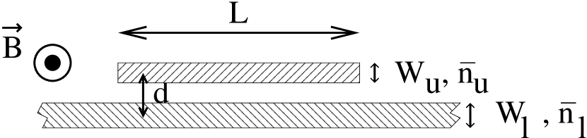
Figure 1: Schematic geometry of electron tunneling between two parallel quantum wires. Electrons are assumed to tunnel between an infinitely long lower wire and a short upper wire of length $L$. The wires are separated by a center-to-center distance $d$. The upper (lower) wire has a width $W_{u}$ ($W_{l}$) and an average electron density $\bar{n}_{u}$ ($\bar{n}_{l}$). A magnetic field $\vec{B}$ is applied perpendicular to the plane of the wires to allow a field-dependent momentum boost $\hbar q_{B}=eBd$ in the tunneling. The energy of the tunneling electrons can be changed by adjusting the voltage applied between the two wires. In the experiments of Ref. [Auslaender et al., 2002], $d=30$ nm, $W_{u}$=20 nm, $W_{l}$=30 nm and $L=2-10\,\mu$m. Electron densities can range $\bar{n}=0-100\,\mu$m^-1. For much of this paper we will assume $(\bar{n}_{l}a_{B})^{-1}\ll 1$ and $(\bar{n}_{u}a_{B})^{-1}\gg 1$, where $a_{B}$ is the Bohr radius, so that the upper wire is close to the Wigner crystal regime and the lower wire can be treated as non-interacting.

In any case, inspired by the results of Steinberg et al.,Ste ; Auslaender et al. (2005) we have been led to consider the theory of momentum-resolved tunneling into a short quantum wire, containing a small number of electrons. We consider tunneling from an infinite lower wire into a short upper wire, under conditions where the energy levels of the upper wire are discrete, and the temperature is small, at least compared to the Coulomb blockade energy and the Fermi energy in the upper wire. We will be particularly interested in the situation where the density in the upper wire is small, so that when two electrons come close together, the electron-electron repulsion is strong compared to the average kinetic energy, and it is difficult for two electrons to change places. At low densities, it can be helpful to think about the one-dimensional electron system as a kind of fluctuating Wigner crystal,Tanatar et al. (1998); Glazman et al. (1992) with a Heisenberg antiferromagnetic exchange couplingHäusler et al. (2002); Matveev (2004a, b) $J$ between successive spins that is small compared to the energy for short-wavelength charge fluctuations or the original Fermi energy. Long-range interactions are expected to enhance the Wigner crystal-like correlations,Schulz (1993) and further reduce $J$.

For a finite low-density system, we can go one step further and consider a situation where $J$ is so small that the temperature $T$ can be larger than $J/k_{B}$ but still small compared to the lowest energy charge excitation, whose energy is proportional to the charge-propagation velocity divided by the length of the wire. This situation, which we denote the “free-spin regime,” will be considered in this paper, along with the strict low-temperature regime (the “ground-state tunneling regime”) where $k_{B}T$ is small compared to all excitation energies. We shall also discuss a situation $k_{B}T\gg NJ$, in which $k_{B}T$ is larger than all spin excitation energies, including multiple spin excitations, which we shall refer to as the “extreme free-spin regime.” We shall further distinguish between a “true Wigner crystal” and a “fluctuating Wigner crystal” depending on whether the root-mean-square displacement of an electron in the center of a finite wire, due to quantum fluctuations, is smaller or larger than the mean electron spacing.

In our discussion, we shall treat the infinite lower wire as a collection of non-interacting electrons. See Fig. 1. Interactions between the two wires are considered only in so far as the lower wire may act as an ideal conductor that contributes to a frequency-independent screening of the Coulomb interaction between electrons in the upper wire. The high-density end-sections of the upper wire are taken into account only as weakly coupled leads, which set the chemical potential in the confined central part of the wire.

We shall concentrate on tunneling in the limit of zero bias voltage, and shall examine both the momentum dependence (i.e., the dependence on applied magnetic field) and the overall magnitude of the tunneling conductivity, when the gate voltage is adjusted to give degeneracy between the ground states of the upper wire for $N$ and $N-1$ particles. Much of our discussion will focus on cases where $N$ is quite small, but we shall also consider the behavior as $N$ becomes large.

We assume that the coupling of the upper wire to its leads is weak enough that the resulting level broadening is small compared to the thermal energy $k_{B}T$. However, we assume that the conductance between the upper and lower wires is weaker still, so that the resistance is dominated by the tunneling conductance, and so we can calculate the current using Fermi’s golden rule, in which the tunneling matrix element enters only to second order, as a prefactor to the overall conductivity.

This paper is organized in the following way. In Sec. II we introduce the basic model and notation that we use throughout the paper. In Sec. III we discuss the important special case of non-interacting electrons in the upper wire. In Sec. IV we prove some general theorems about the momentum structure of the tunneling for small $N$. In Sec.V we present a numerical study of the double wire geometry, including interwire screening effects, for small $N$ based on exact diagonalization. In Sec. VI we discuss the general features expected for tunneling in the limit of large $N$, focusing on the free-spin regime, where the interactions are very strong and the temperature is large compared to the spin exchange energies. In Sec. VII we compare our theoretical findings with the measurements by Steinberg et al.,Ste ; Auslaender et al. (2005) before summarizing the paper in Sec. VIII.

II Model and notation

The Hamiltonian for electrons in the upper wire consists of a kinetic energy, a one-body confining potential $U(x)$, and a two body interaction $v(x-x^{\prime})$, where $x$ is the distance along the wire. We shall discuss some theorems, below, which are independent of the detailed form of $U$ and $v$. In our more detailed calculations, however, we shall concentrate on the case where $U$ contains infinite vertical walls at $x=0$ and $x=L$, together with a potential arising from a uniform positive background in the interval $0<x<L$. The interaction $v$ will have the form of a Coulomb potential at intermediate distances, screened at long distances by the parallel lower wire, and cut off at short distances because of the finite thickness of the upper wire. With these choices, one can consider a limit $N\to\infty,L\to\infty$ with $N/L$ fixed, and the electrons will be uniformly spread along the wire. We shall primarily be concerned, however, with systems where $N$ is not very large.

Let $\Psi^{N}_{\alpha}$ and $\Psi^{N-1}_{\gamma}$ represent many body states of the upper wire with $N$ and $N-1$ electrons, respectively, with energies $E^{N}_{\alpha}$ and $E^{N-1}_{\gamma}$. We consider here the case where the voltage $V$ between the upper and lower wire is small compared to $k_{B}T$, and the tunneling conductance may be written as $G=G_{+}+G_{-}$ in terms of

$$G_{\pm}=C\mathcal{B}(k_{\pm})\;,$$ (1)

where

$$\mathcal{B}(k)=\sum_{\alpha\gamma\sigma}|\langle\Psi^{N}_{\alpha}|c^{\dagger}_{k\sigma}|\Psi^{N-1}_{\gamma}\rangle|^{2}w_{\alpha\gamma}\;,$$ (2)

$$w_{\alpha\gamma} =e^{-\beta[E^{N-1}_{\gamma}-\mu(N-1)]}f(\epsilon_{\alpha\gamma})$$

$$=e^{-\beta(E^{N}_{\alpha}-\mu N)}[1-f(\epsilon_{\alpha\gamma})]\;,$$ (3)

$$\epsilon_{\alpha\gamma}=E^{N}_{\alpha}-E^{N-1}_{\gamma}\;,$$ (4)

$$C=\frac{\pi e^{2}}{2\hbar}\lambda^{2}\beta\nu L\frac{e^{-\beta\mu N}}{Z_{N}+e^{-\beta\mu}Z_{N-1}}\;,$$ (5)

and $c^{\dagger}_{k\sigma}=\int_{0}^{L}dx\psi^{\dagger}_{\sigma}(x)e^{ikx}/\sqrt{L}$ creates a particle in the upper wire with spatial wave function $e^{ikx}$ and spin $\sigma=\pm 1/2$, while $\nu$ is the (total) density of states per unit length at the Fermi energy of the lower wire, $\lambda$ is the coefficient of the tunneling Hamiltonian (properly normalized), $\mu$ is the chemical potential, $\beta=1/(k_{B}T)$, $f(\epsilon)=1/\{1+\exp[\beta(\epsilon-\mu)]\}$ is the Fermi function, and $Z_{N}$ is the partition function of the upper wire when it contains precisely $N$ electrons. (We neglect the probability of occupancies other than $N$ or $N-1$.) $k_{\pm}$ are given by the lower wire wavevectors at the Fermi energy, shifted by the perpendicular magnetic field $B$:

$$k_{\pm}=\pm k_{F}^{l}+eBd/\hbar\;.$$ (6)

In the limit where $k_{B}T$ is small compared to any excitation energies of the system, only the ground states contribute to the sum in (2), and one obtains a large value of $G$ only if the gate potential is adjusted so that $E^{N}-E^{N-1}-\mu$ is close to zero, i.e., of order $k_{B}T$ or smaller. If $E^{N}-E^{N-1}=\mu$ precisely, we have

$$G_{\pm}=\frac{\pi e^{2}}{4\hbar}\lambda^{2}\beta\nu L\frac{1}{g_{N}+g_{N-1}}\mathcal{\tilde{B}}(k_{\pm})\;,$$ (7)

where

$$\mathcal{\tilde{B}}(k)=\sum_{\alpha\gamma\sigma}|\langle\Psi^{N}_{\alpha}|c^{\dagger}_{k\sigma}|\Psi^{N-1}_{\gamma}\rangle|^{2}\;,$$ (8)

and $g_{N}$ and $g_{N-1}$ are the degeneracies of the ground states $\Psi^{N}$ and $\Psi^{N-1}$.

For the system under consideration, with spin-independent interactions and no spin-orbit effects, eigenstates of the Hamiltonian will have a definite quantum number for the total spin $S$. In the absence of a Zeeman field, then, the $N$-electron ground-state will have a degeneracy $g_{N}=(2S_{N}+1)$, where $S_{N}$ is the corresponding spin quantum number. The indices $\alpha$ and $\gamma$ may then be chosen to label states with different values of the spin component $S_{z}$. In the case where there is an applied magnetic field with a Zeeman energy large compared to $k_{B}T$, however, the degeneracy will be removed, and we need only consider the states with spins aligned parallel to the field, $S_{z}=S$.

When the Zeeman field is absent, we may use the Wigner-Eckart theorem to carry out the sum over the spin indices, and write

$$\mathcal{\tilde{B}}(k)=D|M(k)|^{2}\;,$$ (9)

where $M$ is the matrix element

$$M(k)=\langle\Psi^{N}_{\alpha}|c^{\dagger}_{k\sigma}|\Psi^{N-1}_{\gamma}\rangle\;,$$ (10)

with the indices for $S_{z}$ chosen as $\alpha=S_{N}$ and $\gamma=S_{N-1}$, and $\sigma=\alpha-\gamma$. The constant $D$ is given by

$$D=1+2\max(S_{N},S_{N-1})\;.$$ (11)

In order to have a non-zero matrix element, we must have $|S_{N}-S_{N-1}|=1/2.$ This condition is always satisfied for the ground states, because for a system obeying the one-dimensional Schrödinger Equation with spin-independent interactions, the lowest energy state necessarily has spin quantum number $S=0$, if $N$ is even, and $S=1/2$, if $N$ is odd, according to the Lieb-Mattis theorem.Lieb and Mattis (1962) This theorem also tells us that $D=2$ for tunneling between ground states.Lie

It is instructive to define a “quasi-wavefunction”

$$\Psi^{N}_{\rm eff}(x)\equiv\langle\Psi^{N-1}_{\gamma}|\psi_{\sigma}(x)|\Psi^{N}_{\alpha}\rangle\;,$$ (12)

so that $M(k)=\int dxe^{ikx}\Psi^{N*}_{\rm eff}(x)/\sqrt{L}$. For non-interacting electrons, $\Psi^{N}_{\rm eff}(x)$ is the wave function for the last added electron, and its norm is 1. For interacting electrons, the norm will be less than 1, due to orthogonality catastrophe-type effects.

We remark that the value of $G$ given by equation (7) is not actually the maximum value of the conductance that can be achieved at the given temperature $T$. A somewhat larger conductance can be achieved by shifting the gate voltage slightly away from the value where the states for $N$ and $N-1$ particles have precisely the same energies, in order to take advantage of the differing degeneracies of the states. One finds that the maximum conductance is related to $G$ in Eq. (7) by

$$G_{\rm max}/G=2(\eta^{2}+1)/(1+\eta)^{2}\;,$$ (13)

where $\eta=(g_{N}/g_{N-1})^{1/2}$. The maximum occurs when $E^{N}-E^{N-1}-\mu=k_{B}T\ln\eta$, so that there is equal probability for the upper wire to have $N$ or $N-1$ electrons. For ground-state tunneling between states with spins 0 and 1/2, the correction factor for the maximum conductance is $G_{\rm max}/G=1.0294$.

If the spin excitation energies are sufficiently low compared to all other excitation energies, we may consider tunneling in the “extreme free-spin” regime, where $k_{B}T$ is large compared to the spin energies, and we may neglect the energy differences between different spin states. The degeneracy factors in the expression for $C$, Eq. (5), are then given by $g_{N}=2^{N}$, and the labels $\alpha$ and $\gamma$ in the equation for $\mathcal{\tilde{B}}(k)$, Eq. (2), must be summed over all of the states in the manifold.

In the formulas above, we have assumed that the localized section of the upper wire is separated from its high-density leads by barriers sufficiently high that the level width $\Gamma$ due to coupling to the leads is small compared to $k_{B}T$. In the other limit, where $k_{B}T\ll\Gamma$, the prefactor $C$ for ground-state tunneling will be proportional to $\Gamma^{-1}$ rather than $T^{-1}$. If $eV$ is larger than both $k_{B}T$ and $\Gamma$, then we cannot use the linear conductance formulas, but the dependence of the current on momentum transfer should still be proportional to $\mathcal{\tilde{B}}(k)$ at moderate voltages.

III Non-interacting electrons

It is useful to begin by recalling some results for non-interacting electrons. We consider particularly the case of square-well confinement, where $U(x)=0$ for $0<x<L$, and $\infty$ otherwise. The one-electron states are then sine waves, with spatial dependence $\phi_{N}(x)=(2/L)^{1/2}\sin[k_{\tilde{N}}x]$, where $k_{\tilde{N}}=\tilde{N}\pi/L$ , and, in the absence of a Zeeman field,

$$\tilde{N}=\left[\frac{N+1}{2}\right]_{\rm Int}\;,$$ (14)

with $[X]_{\rm Int}$ the integer part of $X$. For fully polarized electrons (or spinless fermions), we have simply $\tilde{N}=N$. In either case, one finds that

$$M(k)= e^{ikL/2}\frac{\sqrt{2}i^{\tilde{N}-1}}{L}\Biggl{[}\frac{\sin[(k+k_{\tilde{N}})L/2]}{k+k_{\tilde{N}}}$$

$$-(-1)^{\tilde{N}}\frac{\sin[(k-k_{\tilde{N}})L/2]}{k-k_{\tilde{N}}}\Biggr{]}\;.$$ (15)

We note that the matrix element vanishes at $k=0$ if and only if $\tilde{N}$ is even.

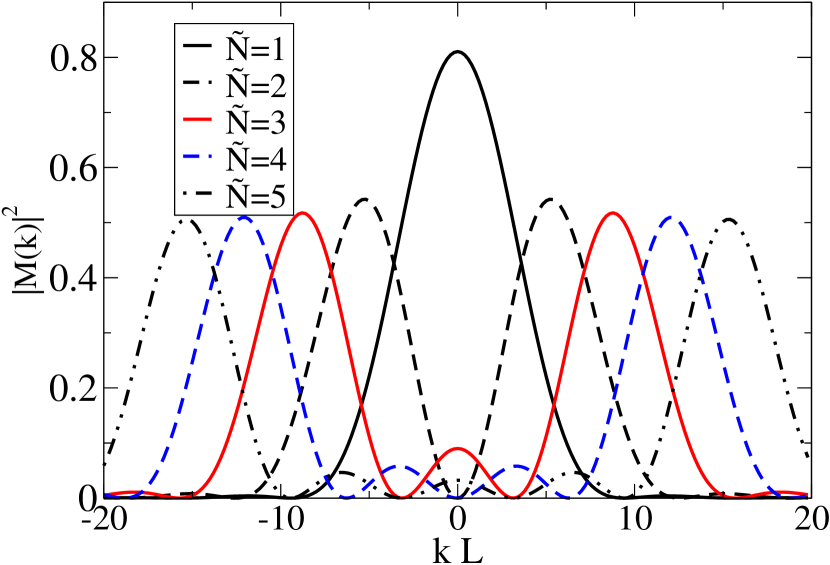
Figure 2: (Color online.) Momentum resolution of one-particle box states. Shown is the modulus squared of Eq. (III) for various values of $\tilde{N}$. Many of the features in the non-interacting case remain when interactions are included and the Fourier transform of a many-body wavefunction is taken.

For large $N$, we see in Fig. 2 that $|M(k)|^{2}$ has sharp maxima at $k=\pm k_{\tilde{N}}$, which become $\delta$-functions in the limit $N\to\infty,\;L\to\infty$. Of course, $k_{\tilde{N}}$ corresponds to the Fermi momentum of the infinite system. For large but finite $N$, the $\delta$-functions broaden into diffraction patterns, with spacing $\delta k=2\pi/L$ between successive zeroes, and a peak-width of the same order.

Tserkovnyak et al.Tserkovnyak et al. (2002, 2003) have discussed the form of $M(k)$ for large but finite $N$ when the confinement at the end of the wires is soft on the scale of the Fermi wavelength. In this case they find an asymmetric diffraction pattern, which falls off rapidly for $|k|>k_{\tilde{N}}$, but relatively slowly on the side $|k|<k_{\tilde{N}}$. The spacing between zeroes is not constant and is slightly larger than $2\pi/L$.

IV Some theorems for small systems

Some rigorous theorems are helpful for understanding the properties of $\mathcal{\tilde{B}}(k)$, particularly at small values of $N$.

As a consequence of time-reversal invariance, all wave functions may be chosen to be real. From this it follows that $\mathcal{\tilde{B}}(k)=\mathcal{\tilde{B}}(-k)$. Also, the matrix element $M(k)$, which determines $\mathcal{\tilde{B}}(k)$ in the case of ground state tunneling, satisfies $M(k)=M(-k)^{\ast}$.

If the confining potential is symmetric about the center of the well, the states $\Psi^{N}$ and $\Psi^{N-1}$ may be classified by their parity under inversion through the center of the well. If the states have the same parity, then $M(k)=M(-k)$, and hence $M$ must be real. If the states have opposite parity, then $M(k)=-M(-k)$, and $M$ must be purely imaginary. In either case, if $M(k)$ changes sign, as a function of $k$, there will be one or more values of $k$ where $M(k)=0$. Thus, in the ground-state tunneling regime, there can be points $k$ where $\mathcal{\tilde{B}}(k)=0$. We have already seen an example in the case of non-interacting electrons.

For the case $N=1$, the ground state wave function can be written in first quantized notation (in terms of position $x$ and spin index $\sigma$), as

$$\Psi_{\alpha}(x,\sigma)=\Psi(x)\delta_{\sigma,\alpha}\;,$$ (16)

where $\Psi(x)>0$ for all $x$. (This is true regardless of whether or not the confining potential has inversion symmetry.) Thus, for the case $N=1$, the matrix element $M$ can be written as

$$M(k)=\int dx\frac{e^{ikx}}{\sqrt{L}}\Psi^{*}(x)\;.$$ (17)

Clearly, $|M(k)|$ has its maximum when $k=0$, for $N=1$.

We obtain a similar behavior for ground-state tunneling in the case $N=2$. The ground state of the two-fermion problem, in any number of dimensions, is always a spin-singlet, with a spatial wave function that has no nodes. Thus, for $N=2$ we may write, in first-quantized notation,

$$|\Phi\rangle=f(x_{1},x_{2})\chi_{0}(\sigma_{1},\sigma_{2})\;,$$ (18)

where $\chi_{0}=2^{-1/2}(|\uparrow\downarrow\rangle-|\downarrow\uparrow\rangle)$, while $f$ is real and positive, and symmetric under interchange of its arguments. We may also write

$$c^{\dagger}_{k\downarrow}|\Psi_{\uparrow}\rangle=\frac{1}{\sqrt{2L}}[e^{ikx_{2}}\Psi(x_{1})\ |\uparrow\downarrow\rangle-e^{ikx_{1}}\Psi(x_{2})\ |\downarrow\uparrow\rangle]\;,$$ (19)

where $\Psi(x)>0$ is the wave function for the one-particle system. The matrix element $M(k)$ is then given by

$$M(k)=\int dx_{1}dx_{2}\frac{e^{ikx_{2}}}{\sqrt{L}}\Psi(x_{1})f(x_{1},x_{2})\;,$$ (20)

which clearly has its maximum at $k=0$.

The situation is different if we consider tunneling between the $N=1$ system and the lowest triplet state of the $N=2$ system. If we choose the spins to be maximally aligned in the $z$-direction, we have

$$|\Phi\rangle=g(x_{1},x_{2})|\uparrow\uparrow\rangle,$$ (21)

and

$$c^{\dagger}_{k\uparrow}|\Psi_{\uparrow}\rangle=\frac{1}{\sqrt{2L}}[e^{ikx_{2}}\Psi(x_{1})-e^{ikx_{1}}\Psi(x_{2})]\ |\uparrow\uparrow\rangle\;,$$ (22)

where $g$ is antisymmetric under interchange of its arguments, and

$$M(k)=\sqrt{2}\int dx_{1}dx_{2}\frac{e^{ikx_{2}}}{\sqrt{L}}\Psi(x_{1})g(x_{1},x_{2})\;.$$ (23)

If the confining potential is symmetric, then $g$ will be antisymmetric under inversion, while $\Psi$ is symmetric. It follows that $M=0$ at $k=0$, and $|M(k)|$ will have its maximum at a non-zero value of $k$.

The triplet state will be the actual ground state of the $N=2$ system if there is an applied Zeeman field large enough to overcome the exchange splitting between the singlet and triplet states. It is also the correct ground state for a model of spinless fermions. In the absence of a Zeeman field, in the free-spin regime, where the temperature is larger than the exchange splitting, but smaller than all other excitation scales, the quantity $\mathcal{\tilde{B}}(k)$ will have two contributions from the singlet state and four contributions from the triplet. In this case, the function $\mathcal{\tilde{B}}(k)$ will not be zero at $k=0$, but we may have a situation with $\mathcal{\tilde{B}}(k)$ having a local minimum at $k=0$, with a pair of maxima at a finite value of $|k|$, as in Fig. 10 below.

For $N=3$, the many-body ground state for non-interacting electrons in symmetric confinement has odd parity under inversion, as it has two electrons in the lowest even-parity level, and one electron in the second odd-parity level. The $N=4$ state has even parity. These parities cannot be altered by a weak electron-electron interaction, and it is likely that they will hold even for rather strong interactions. As we have seen, the ground state for $N=2$ has even parity. Consequently, for electrons in a symmetric confining potential, the ground state tunneling form factor $\mathcal{\tilde{B}}(k)$ should vanish at $k=0$ for $N=3$ and $N=4$ .

The feature of a zero amplitude at $k=0$ does not persist, if the confining potential is not symmetric under inversion. For a sufficiently asymmetric potential there need not be even a local minimum near $k=0$. For example in the case of an asymmetric double-well potential, when there is little overlap between the wave functions in the two wells, one would expect that $\mathcal{\tilde{B}}(k)$ for $N=3$ and $N=4$ should be qualitatively similar to the form for $N=1$ and $N=2$.

The state $N=5$ has even parity, at least for weakly interacting electrons. Thus the matrix element for tunneling between the ground states with 4 and 5 electrons will be non-zero at $k=0$. For non-interacting electrons, $\mathcal{\tilde{B}}(k)$ has a local maximum at $k=0$, but has its absolute maxima at a non-zero value of $|k|$, with zeroes of the amplitude in between. See Fig. 2. We expect these qualitative features for non-interacting electrons to persist for strong interactions in small-$N$ wires.

We now turn to exact numerics for small $N$.

V Calculations for $N=1$ to $4$

We can illustrate some of the ideas and results discussed in Sec. IV with exact numerical calculations for small $N$ which take into account finite size and screening effects from the lower wire.

V.1 Form of electron interaction

We assume the interaction potential is a Coulomb interaction with both a short and a long range cutoff. The short range cutoff is achieved in a simple way by modifying a $\frac{1}{z}$ potential to $\frac{1}{\sqrt{z^{2}+W^{2}}}$ where $z=x-x^{\prime}$ is the separation of two electrons along the wire and $W$ is a short range cutoff ($W_{u}$ for the upper wire), which is roughly the width of the quantum wire. The long range cutoff, with experiments by Steinberg et al.Ste ; Auslaender et al. (2005) in mind, is achieved by putting a second, lower wire with width $W_{l}$, assumed to be perfectly conducting, parallel to the system under study, at center to center distance $d$. See Fig. 1. This approximation is valid, strictly speaking, if the electron density in the lower wire is sufficiently high that many modes are occupied, while there is only one mode occupied in the central region of the upper wire. We note that for the experiments of Ref. [Ste, ; Auslaender et al., 2005], there are at most only a few modes occupied in the higher density wire, so the assumptions made here may overestimate the quality of screening actually obtained in the experiments.

Let $V_{0}(z,W)=\frac{e^{2}}{\epsilon}\frac{1}{\sqrt{z^{2}+W^{2}}}$ be the interaction with short range cutoff $W$ between particles separated by a distance $z$. Here $\epsilon$ is the dielectric constant. The energy distribution of the wires in Fourier space can be estimated as:

$$E= \frac{1}{2}\int dq\biggl{[}\delta\rho_{u}(q)\delta\rho_{u}(q)\tilde{V}_{0}(q,W_{u})+\delta\rho_{l}(q)\delta\rho_{l}(q)\tilde{V}_{0}(q,W_{l})$$

$$+2\delta\rho_{u}(q)\delta\rho_{l}(q)\tilde{V}_{0}(q,d)\biggr{]}\;,$$ (24)

where $\delta\rho_{u/l}(q)$ is the net charge density (electron density minus background positive charge) of the upper/lower wire in Fourier space and $\tilde{V}_{0}(q,W_{u}/W_{l})$ is the Fourier transform of the interaction (already with the short range cutoff) within the upper/lower wire. Taking the variation with respect to the lower wire charge density $\delta\rho_{l}$:

$$\frac{dE}{d(\delta\rho_{l})}=\delta\rho_{l}(q)\tilde{V}_{0}(q,W_{l})+\delta\rho_{u}(q)\tilde{V}_{0}(q,d)\;.$$ (25)

Setting it to zero,

$$\delta\rho_{l}(q)=-\frac{\delta\rho_{u}(q)\tilde{V}_{0}(q,d)}{\tilde{V}_{0}(q,W_{u})}\;.$$ (26)

Putting this back into (V.1) and taking out the common factors of $\delta\rho_{u}^{2}$,

$$E=\frac{1}{2}\int\delta\rho_{u}^{2}(q)\left[\tilde{V}_{0}(q,W_{u})-\frac{\tilde{V}_{0}^{2}(q,d)}{\tilde{V}_{0}(q,W_{l})}\right]dq\;.$$ (27)

Comparing this with the form of self interaction in the upper wire it is easy to see the effective form of interaction in Fourier space is

$$\tilde{V}_{\rm eff}(q)=\tilde{V}_{0}(q,W_{u})-\frac{\tilde{V}_{0}^{2}(q,d)}{\tilde{V}_{0}(q,W_{l})}\;,$$ (28)

where we have made explicit reference to the short distance cut off in real space: $\tilde{V}_{0}(q,W)=\int_{-\infty}^{\infty}dx\frac{e^{iqx}}{\sqrt{x^{2}+W^{2}}}$. The interaction (28) is plotted in real space in Fig.3.

Figure 3: Effective interaction potential $V_{\rm eff}$, as a function of the separation $z$ between two electrons in the upper wire, taking into account the finite width $W_{u}$ of the upper wire and screening due to a parallel lower wire of width $W_{l}$ at a distance $d$. See Fig. 1. Dashed and dotted lines show the bare Coulomb interaction $z^{-1}$, and the unscreened interaction softened at short distances, $1/\sqrt{z^{2}+W_{u}^{2}}$. Parameters are $d=1$, $W_{u}=0.1$ and $W_{l}=0.15$. Region $0<z<0.5$ is expanded in the inset. In the main plot $1/z$ and $1/\sqrt{z^{2}+W_{u}^{2}}$ are indistinguishable in the range $0.5<z<4$. In the inset the interaction potential $V_{\rm eff}(z)$ and $1/\sqrt{z^{2}+W_{u}^{2}}$ are indistinguishable in the range $0<z<0.5$.

V.2 Model for confinement and background charge distribution

We now consider the model of a few interacting electrons in a box of length $L$. A uniform positive background with density equal to the average electron density is added to maintain charge neutrality. The resulting one-body potential $U(x)$ takes the following form:

$$U(x)=\left\{\begin{array}[]{ll}\infty,&\textrm{if $x<0$ or $x>L$},\\ -\bar{n}\int_{0}^{L}V_{\rm eff}(x-x^{\prime})dx^{\prime},&\textrm{if $0<x<L$}.\end{array}\right.$$ (29)

Here $\bar{n}$ is the density of positive background charge. When the electron number $N$ is fixed, $\bar{n}=N/L$. When the electron density changes, as in the case of tunneling into a relatively rigid box, $\bar{n}$ is taken to be the average of the initial and final electron density. The precise value of $\bar{n}$ does not qualitatively change the results discussed below.

Systems with up to four electrons, both with and without spin, were solved by directly diagonalizing the exact many-body Hamiltonian using the Lanczos method.Dagotto (1994); Cullum and Willoughby (1985) Earlier applications of the Lanczos method to one-dimensional quantum dots were reported in Refs. [Häuseler and Kramer, 1993; Jauregui et al., 1996, 1993] , by Häusler and Kramer, and collaborators. Energy spectra for up to $N=4$ particles, with Coulomb interactions unscreened at large distances, were presented in Ref. [Jauregui et al., 1993], and the splitting between the lowest energy singlet and triplet states was found to fall off rapidly with increasing wire length in this case. Density distributions for up to four particles, and density correlation functions for three particles, were obtained in Ref. [Jauregui et al., 1993]. Matrix elements for tunneling were discussed, and tunneling rates were computed, in Ref [Jauregui et al., 1996], but only for the incoherent case, with no momentum conservation. The parameters of the calculation, including the interaction strength and the geometry of two parallel wires with one screening the other, were obtained from estimates in the experiments by Steinberg et al..Ste ; Auslaender et al. (2005) In the calculation shown here we take the upper wire width $W_{u}$ to be 20 nm, the lower wire width $W_{l}$ to be 30 nm and the center to center distance $d$ between wires to be 31 nm. The interaction strength between electrons is obtained by using the dielectric constant of GaAs, $\varepsilon=13.1$, and effective mass $m^{*}=0.067m_{\rm{e}}$, which gives a Bohr radius $a_{B}=\varepsilon\hbar^{2}/(m^{*}e^{2})\approx 10$ nm.

V.3 Ground state density and density-density correlation

Before discussing the momentum structure of the tunneling matrix element, a discussion of ground state properties is useful. In the case of electrons with spin, as discussed before, the ground state has total spin $0$, for a system with an even number of electrons, and total spin $1/2$, for a system with an odd number of electrons. As the electron density decreases, there is a relative increase in the importance of the potential energy compared to the kinetic energy, and there is a crossover from a relatively uniform liquid state into a Wigner crystal-like state with spatially localized electrons. This crossover can be seen in Figs. 4 and 4 where we plot the ground state density distribution and the density-density correlation function for a system of $N=4$ electrons.

Figure 4: Top: Ground state density of a four electron system with spin. Scaled densities are measured in units of $1/L$. In the label of the individual plot, “density” means the average physical density $N/L$ of the system, in units of $\mu\rm{m}^{-1}$. Bottom: Ground state density-density correlation of a four electron system with spin. The density-density correlation function is defined as $\frac{1}{1-x}\int_{0}^{1-x}\rho(x^{\prime})\rho(x^{\prime}+x)dx^{\prime}$. The pre-factor before the integral is to take into account the finite length of the system.

In Fig. 4, at a large physical density of twenty-one electrons per micron, the scaled electron density distribution has smooth variation with spatial frequency $2k_{F}$, which is simply a Friedel oscillation resulting from boundary effects. At the lowest density of one electron per micron, the scaled electron density has distinct peaks, whose number equals that of the electrons in the system, corresponding to a $4k_{F}$ Wigner crystal density variation. The signature of Wigner crystal correlations is also clearly seen in Fig. 4, in the form of $4k_{F}$ oscillations in the density-density correlation function at low physical density.

The behavior of spinless electrons and spin polarized electrons is significantly different from the case with spin (shown in Fig. 4) in its spin-singlet ground state. As shown in Fig. 5, contrary to the case of a system with spin, decreasing the physical density does not significantly alter the ground state.

Figure 5: Top: Ground state density of a four electron system without spin. Bottom: Ground state density-density correlation of a four electron system without spin. See Fig. 4 for a definition of the density-density correlation function.

Neither the scaled electron density distribution nor the density-density correlation function changes more than ten percent when the physical density changes over an order of magnitude from twenty-one to one electron per micron. This means that the spinless system is Wigner crystal-like, although essentially non-interacting for all densities and gate potentials. This is the result of a combination of the Pauli Exclusion Principle, the cutoff of the interaction at large distances due to the second perfectly conducting (lower) wire, and the actual parameters of the experimental system. When the density is high and inter-particle distance $z\ll a_{B}$, the interaction energy is much smaller than kinetic energy. When the density is low and average inter-particle distance $z\gg d$, the interaction becomes effectively short-ranged due to screening, diminishing its effect because in the spinless model the wavefunction vanishes when electrons come together.

As mentioned before, in the experiments of Steinberg et al.,Ste ; Auslaender et al. (2005) $a_{B}\approx 10$ nm and $d\approx 30$ nm. Define $r_{s}\equiv\ a/a_{B}$, where $a$ is the average inter-particle distance. Then, for $r_{s}\gtrsim 3$, the long range cutoff set by screening from the second wire kicks in and starts to strongly suppress interaction effects. Our numerical calculations confirm this picture. Since long range interactions are important in establishing Wigner crystal-like correlations,Schulz (1993) screening from the lower wire acts to inhibit somewhat Wigner crystal-like correlations. Longer range interactions tend to make the peaks in the ground state density distribution and in the density-density correlation more prominent. Although the effect of the decrease in physical density is small in the spinless case, we can see in Fig. 5 that distinct peaks in ground state density are most prominent in the intermediate physical density of eleven electrons per micron. Fig. 5 also shows that at a density of eleven electrons per micron, the electrons more strongly avoid each other than at both higher and lower density. Nevertheless, even at intermediate densities our numerical results show that with experimental parameters of Steinberg et al.,Ste ; Auslaender et al. (2005) the interaction effect would be quite weak for spin polarized electrons.

We note that numerical results for the electron density and correlation function qualitatively similar to ours (inter-wire screening effects not considered) were obtained in Ref. [Szafran et al., 2004].

V.4 Momentum dependent tunneling matrix element

Let us now consider tunneling between the interacting electron system and a non-interacting electron system, shown schematically in Fig. 1. Here we consider the situation when the initial and final states of the interacting electron system (upper wire) are both ground states. As discussed in Sec. II, the tunneling probability is then proportional to the matrix element $|M(k)|^{2}$.

Figure 6: Top: Squared matrix elements of tunneling from a two to three electron system with spin vs. scaled wavevectors $kL/\pi$. Here the $L=0.1\,\mu$m curve is indistinguishable from non-interacting limit. Bottom: Same as Top only tunneling from three to four electrons.

Figure 7: Top:Squared matrix elements for tunneling from a two to three electron spinless system vs. scaled wavevectors $kL/\pi$. Bottom: Same as Top only tunneling from three to four electrons.

Typical results of the square of the absolute value of tunneling matrix element $M$ are shown in Fig. 6 for electrons with spin and in Fig. 7 for electrons without spin. All results are symmetric under the interchange $k\to-k$. Note that the case with spin shows a much greater change with density, although this appears to be limited mostly to the amplitude of the peak in the tunneling.

It is clear from the discussion of previous passages that the spinless system ground state under any density can be effectively described using a non-interacting model. This is clearly seen in the plots. In the spinless model, to get the noninteracting matrix element tunneling from $N-1$ to $N$ electron ground state we put $k_{\tilde{N}}=\pi N/L$ in Eq (III). Manifestly, this has the consequence that $M(k=0)$ is zero for even $N$ and non-zero for odd $N$, and this is seen in the numerical result. There is also a sharp maximum near $k_{\tilde{N}}=\pi N/L$. As $N\rightarrow\infty$, this maximum will approach $k_{\tilde{N}}$. All these features are seen in Figs. 7. The insets of the two plots further demonstrate what has already been discussed at the end of the previous subsection: Electron interactions cause greatest deviation of $|M(k)|^{2}$ from its non-interacting limit at intermediate density. At both very large and small density $|M(k)|^{2}$ approaches the non-interacting limit.

For systems with spin, the interaction has a more significant effect on the matrix element. Yet the salient feature here remains that, even at very low density and strong interaction, and even after the system changes from a Fermi liquid-like state to a Wigner crystal-like state, the qualitative features of the scaled matrix element remain similar to those of non-interacting solutions: The positions of the maxima are only slightly shifted, the positions of zeros a bit more so (apart from $k=0$), and the values of the maxima are reduced by no more than $30\%$ relative to the non-interacting case, for densities down to $1\,\mu{\rm m}^{-1}$. Furthermore, since for $N=3$ and $N=4$, the systems with spin have the same matrix element in the non-interacting limit, the overall features of the tunneling matrix elements, after scaling, are very similar, even with interactions.

V.5 Spin exchange energy

In the model with spin, the first excited state has total spin $S=1$ for even numbers of electrons, and while for odd numbers of electrons the situation can be more complicated.Häusler (1996) The energy gap between the ground state and the first excited state decreases as the electron density tends to zero. The high density, low interaction part of this change in the gap can be understood by simple first order perturbation theory using a non-interacting wavefunction, as shown in Fig. 8. In the low density, strongly interacting Wigner crystal-like state, electrons are spatially confined around their equilibrium positions. The system can be approximated as a Heisenberg spin chain, where spin exchange is achieved by tunneling between adjacent sites:Häusler et al. (2002); Matveev (2004b, a)

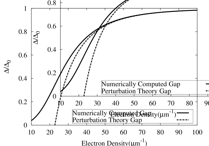
Figure 8: Comparison of the gap $\Delta$ between the ground state and the first excited state energy in a system of two electrons in a box, obtained by direct calculation versus by first order perturbation theory. The unit is $\Delta_{0}$, the non-interacting energy gap between the ground and the first excited state.

Figure 9: Estimate of the spin exchange energy per electron from a two and four electron system using the interaction in Eq. (28). Both of the axes are in physical units: the x-axis is the physical density, in units of one electron per $\mu$m, the y-axis is the physical exchange energy $J$ in units of $\mu$eV. Typical experimental temperatures are in the range 250 mK-2 K $\approx 25\mu$eV-200 $\mu$eV.

$$H_{\rm spin}=J\sum_{i=1}^{N-1}\vec{S}_{i}\cdot\vec{S}_{i+1}\;.$$ (30)

This Hamiltonian describes the energy spectrum of low-lying spin excitations. Specifically, in the case of $N=2$ we simply have

$${}J=\Delta\;,$$ (31)

where $\Delta$ is the gap between the ground state and the first excited state. For $N=4$ numerical solution of the four spin Heisenberg chain gives:

$${}J=1.51777\Delta\;.$$ (32)

Analytical estimates of $J$ have been obtained in Refs. [Matveev, 2004a, b; Häusler, 1996; Kli, ]. Hartree-Fock estimates are given in Ref. [Häusler et al., 2002]. Related estimates of the spin velocity are given in Ref. [Kecke and Häusler, 2004] based on the ladder approximation and in Ref. [Creffield et al., 2001].

Because the tunneling barrier between adjacent sites increases with larger electron-electron interaction strength, the effective Heisenberg exchange constant, and hence the gap between the ground state and the first excited state, will decrease to zero as the physical density goes to zero. It is interesting to note that the effective Heisenberg exchange energy, extracted from the two-electron system and four-electron system gap using Eqs. (31) and (32), closely follow each other in the low density regime, as seen in Fig. 9. This supports our assumption that spin excitations in the low-density regime are well described by a Heisenberg model, and it suggests that in this regime, an estimate of the Heisenberg exchange from an exact calculation of systems with a few electrons can provide a reasonable prediction for the spin velocity of an infinite wire with the same electron density. It should be noted, however, that the numerical value of $J$ may depend sensitively on both short distance and long distance cut offs.Häuseler and Kramer (1993)

V.6 Mixed spin states

In the low density regime, where the spin exchange energy is small, one may encounter an experimental regime where the temperature is larger than $J$, but still small compared to the lowest energy for charge excitations. In that case, the tunneling conductance will be a superposition of the results obtained from different spin states. Also, under experimental conditions, the Zeeman energy $E_{Z}=g_{s}\mu_{B}B$ may be comparable to or larger than $J$. (Here $\mu_{B}$ is the Bohr magneton and $g_{s}$ is the $g$-factor of the electron spin.) If the Zeeman energy is large compared to both $k_{B}T$ and $J$, then the electron system will be fully spin polarized, and calculations for spinless electrons will apply.

As a simplest example, consider the case $N=2$, in the low-density regime. If the temperature and the singlet-triplet splitting $\Delta$ are both small compared to all charge-excitation energies in the $N=1$ as well as in the $N=2$ states, then the sum in Eq. (2) may be restricted to six states: the lowest singlet and triplet states of the $N=2$ system and the two spin states of $N=1$ ground state. As there are only two independent matrix elements involved, the sum may be further simplified to read

$$\mathcal{B}(k)=w_{s}|M_{s}(k)|^{2}+w_{t}|M_{t}(k)|^{2},$$ (33)

where $M_{s}(k)$ and $M_{t}(k)$ are the matrix elements for the singlet and triplet states defined in Eq.(10). The weights $w_{s}$ and $w_{t}$ depend on the Zeeman energy $E_{\rm{Z}}$ and the chemical potential $\mu$, as well as on $\Delta$ and $T$.

In the limit $T\to 0$, the ratio $w_{t}/w_{s}$ will approach either zero or infinity, depending on whether $E_{\rm{Z}}$ is smaller or larger than $\Delta$. In the opposite limit, when $k_{B}T$ is large compared to $E_{\rm{Z}}$ and to $\Delta$, we have $w_{t}/w_{s}\to 3/2$. In Fig.  10, we show the momentum dependence of $\mathcal{B}(k)$ for these three limiting values of $w_{t}/w_{s}$, at $L=0.4\,\mu$m.

To illustrate further, we may consider the case where $\Delta$ is small compared to $E_{\rm{Z}}$ and to $k_{B}T$, but the ratio $E_{\rm{Z}}/(k_{B}T)$ is finite. If $\mu$ is adjusted so that the upper wire has equal probability of having $N=1$ or $N=2$ electrons, then we find

$$\frac{w_{t}}{w_{s}}=\frac{(2x^{2}+5x+2)}{6x},$$ (34)

where $x=\exp[E_{\rm{Z}}/(k_{B}T)]$. As expected, we see that $w_{t}/w_{s}=3/2$, for $x=1$, and $w_{t}/w_{s}\to\infty$, when $x\to\infty$.

Figure 10: Momentum-dependence of tunneling conductance between one-electron and two-electron states for a wire of length $L$=0.4$\mu$m. Dashed curve shows line-shape $|M_{s}(k)|^{2}$ for tunneling into the singlet ground state of the two particle system, applicable at $T=0$ when the Zeeman energy $E_{Z}$ is smaller than the exchange gap $\Delta$. Short-dashed curve shows $|M_{t}(k)|^{2}$, for tunneling into the triplet ground state, applicable at $T=0$ when $E_{Z}>\Delta$. Solid curve is a weighted average, applicable if $T$ is large compared to both $E_{Z}$ and $\Delta$ but small compared to the energy of the lowest charge excitation.

VI Limit of large $N$

Properties of an infinite one-dimensional electron system have been explored by a variety of techniques, including solutions of exactly solvable models, renormalization group methods, bosonization, and conformal field theory. These techniques can be also adapted to the study of finite systems, when $N$ is large.

In this section, we will use mostly bosonization techniques to explore both spin-coherent and spin-incoherent regimes. Bosonization techniques give most readily the electron Green’s functions

$$\mathcal{G}_{\sigma}(x,x^{\prime},t)=\langle\psi_{\sigma}(x,t)\psi_{\sigma}^{\dagger}(x^{\prime},0)\rangle$$ (35)

as a function of position and time $t$. For an infinite system, position variables enter only in the combination $(x-x^{\prime})$, but for a finite system, the distance from the ends may also be important. To obtain the spectral density at a finite energy $\hbar\omega$ (setting $\mu=0$), one must take the Fourier transform with respect to $t$; however one may generally obtain an estimate of this by evaluating $G$ at an imaginary time $\tau$ equal to $\omega^{-1}$. To obtain the ground-state tunneling amplitude for a finite system, when $k_{B}T$ is small compared to all excitation energies, we need to study the Green’s function for $\tau\to\infty$. In particular, if the energies are adjusted so that $E^{N}=E^{N-1}$, then evaluating (35) at a $(N-1)$-electron ground state yields

$$\lim_{\tau\to\infty}\mathcal{G}(x,x^{\prime},\tau)=\Psi^{N}_{\rm{eff}}(x)\Psi^{N\ast}_{\rm{eff}}(x^{\prime}),$$ (36)

where $\Psi^{N}_{\rm{eff}}(x)$ is the quasi-wavefunction defined in Eq. (12). In the free-spin regime, at finite temperatures, we shall make use of a generalization of this result.

VI.1 Ground-state tunneling regime

Numerous works have considered tunneling in the regime where the spin energy is important.Kane et al. (1997); Fabrizio and Gogolin (1995); Kleimann et al. (2002, 2000); Tserkovnyak et al. (2003, 2002); Carpentier et al. (2002); Zülicke and Governale (2002) At sufficiently low energies, an infinite interacting one-dimensional electron system is believed to be described as a Luttinger liquid,Voit (1995) in which spin and charge propagation are characterized by two distinct velocities, $v_{s}$ and $v_{c}$. At finite bias voltages, the amplitude for momentum resolved tunneling into a Luttinger liquid is expected to show structure reflecting both of these velocities. This follows from the form of the one-particle Green’s function ($z=x-x^{\prime}$)

$$\mathcal{G}(z,\tau)\sim\frac{e^{ik_{F}z}}{\sqrt{(v_{s}\tau-iz)(v_{c}\tau-iz)[(v_{c}\tau)^{2}+z^{2}]^{\alpha}}}+{\rm c.c.}\,,$$ (37)

dropping a short-distance cutoff-dependent prefactor. In the limit where the bias voltage $V\to 0$ and $T\to 0$, however, the momentum-resolved tunneling conductance reduces to $\delta$ functions at $k=\pm k_{F}$ similar to that of a non-interacting electron system. The primary effect of the interactions is then to reduce the amplitude of the $\delta$-functions. For an infinite system, the amplitude is predicted to vanish as $\max(k_{B}T,V)^{\alpha}$, when $T$ and $V$ approach 0, where the bulk tunneling exponent $\alpha\geq 0$ depends on the strength of the electron-electron interaction. Tunneling into a point near the end of a semi-infinite system is characterized by a different exponent $\alpha_{\rm{end}}$, which is generally larger than $\alpha$. The tunneling exponents are related to the Luttinger liquid interaction parameter $g$ by $\alpha=(g+g^{-1}-2)/4$ and $\alpha_{\rm{end}}=(g^{-1}-1)/2$ for a single mode wire. Voit (1995) For fermions with repulsive interactions, as considered here, one has $g<1$. For translationally-invariant systems, $g=v_{F}/v_{c}$, where $v_{F}$ is the Fermi velocity with turned off interactions. For not too strong interactions, one can make an RPA estimate for $g$ of a cylindrical wire of radius $R$ with electron density $\bar{n}$ at a distance $D$ from a two-dimensional screening gate:Kane et al. (1997)

$$g^{-1}\approx\sqrt{1+\frac{8\ln(2D/R)}{\pi^{2}\bar{n}a_{B}}}\,.$$ (38)

We remark that if the lower high-density wire had charge modes propagating with a very different velocity from the upper wire, the interwire interactions would not significantly couple or modify the charge modes of individual wires.Matveev and Glazman (1993) Using parameters of Ref. [Ste, ; Auslaender et al., 2005], $2D\approx 1\,\mu$m, $R\approx 20$ nm, $a_{B}\approx 10$ nm, and $\bar{n}\approx 30\,\mu$m^-1 near the localization transition, we get $g\approx 0.3$ which is comparable to the measured $g\approx 0.5$.

Kane, Balents, and FisherKane et al. (1997) considered tunneling into a finite-length metallic carbon nanotube, which has four excitation modes, rather than the single charge and spin modes considered here. Nevertheless, their formulas may be readily adapted to the present case. The general result, for a wire with uniform electron density and hard-wall confinement at the ends, may be written in the form

$$\Psi^{N}_{\rm{eff}}(x)\sim\frac{1}{\sqrt{LN^{\alpha}}}\left[\sin\left(\frac{\pi x}{L}\right)\right]^{\frac{1}{2}(\alpha_{\rm{end}}-\alpha)}\sin(k_{F}x)\;,$$ (39)

valid for positions not too close to the wall where the factors involving $\alpha$ cease to be a good approximation.

As $\alpha$ increases with increasing interaction strength, the overall amplitude of the tunneling matrix element $M(k)$, obtained by Fourier transforming (39), will decrease rapidly with increasing interaction strength, for $N$ large but fixed. However, the momentum-dependence remains qualitatively similar to the form (III) for non-interacting electrons, and the peak at $k_{F}$ broadens only gradually with increasing interaction strength, as illustrated in Fig. 11.

Figure 11: Momentum-dependence of ground-state tunneling for N=10 electrons and various interaction strengths, obtained by calculating $|M(k)|^{2}$ from the effective wavefunction (39). Each curve has been divided by a normalization constant $N_{g}$, chosen so that the plotted curves have equal areas. The norm $N_{g}$ decreases rapidly with increasing interaction strength (decreasing $g$), but the width of the peak broadens only slightly. Note that for $g=1$ the results are equivalent to the $\tilde{N}=5$ case in Fig. 2.

Tserkovnyak et al.Tserkovnyak et al. (2002, 2003) have explored the implications of Luttinger liquid theory for momentum-resolved tunneling into a long finite wire with soft confinement at the ends. Although the emphasis of that work was on tunneling at finite bias, where the discreteness of the energy levels plays a relatively minor role, the analysis can also be applied to estimate the form of $\Psi^{N}_{\rm{eff}}(x)$ and the matrix element $M(k)$ for the ground-state tunneling into a wire with large $N$, for not too strong interactions. Essentially, the factor $\sin(k_{F}x)$ in (39) should be replaced by the WKB wavefunction for a non-interacting electron in a self-consistent potential that gives the correct density profile along the wire. The zeroes of $\Psi^{N}_{\rm{eff}}(x)$ will be spaced further apart near the ends of the wire than near the center, but near the center of the wire, the wavefunctions will look quite similar for the cases of soft and hard confinement. For increasing values of the the electron-electron interaction, the envelope factor in (39) is increasingly weighted towards the center of the wire, so that the Fourier transform $M(k)$ should become correspondingly insensitive to the difference between soft and hard confinement.

VI.2 Finite temperatures

At finite temperatures $T$, for the infinite system, one expects that the $\delta$-functions at $k=k_{F}$ will be broadened by an amount of order $\delta k\approx k_{B}T/(\hbar v_{s})$. If the temperature is larger than the energy of the lowest spin wave mode, $\pi\hbar v_{s}/L$, the broadening will be larger than $2\pi/L$ for a finite system of length $L$. The width $\delta k$ becomes comparable to $k_{F}$ when $k_{B}T$ becomes comparable to $J\sim\hbar v_{s}k_{F}$, the energy of the shortest wavelength spin excitations.

If the spin velocity is very much smaller than the charge velocity, one can enter a regime where $k_{B}T$ is larger than the energy of the shortest-wavelength spin excitations, but still low enough that relatively few short-wavelength charge modes are excited. This regime has been explored in recent papers by Cheianov and Zvonarev,Cheianov and Zvonarev (2004a, b) and by Fiete and Balents.Fiete and Balents (2004) The form factor for momentum-resolved tunneling is indeed broadened by an amount of order $k_{F}$ in this regime, as the Green’s function in position space is found to fall off exponentially with distance. A more precise description of this behavior will be given in the next subsection.

The lowest energy cost for a charge excitation is $\epsilon_{c}=\pi\hbar v_{c}/L$. The highest energy for a spin state with multiple excitations is $\approx N\hbar v_{s}k_{F}$. Earlier, we defined an extreme free-spin regime as having a temperature high enough so that all spin states have equal weight, while there are no charge excitations. This makes sense for a small system, but is very restrictive for a large system, as it requires that $v_{s}/v_{c}\ll 1/N^{2}$. However, the spins will actually be effectively free as long as $k_{B}T$ is greater than the energy of a single short wavelength spin-excitation, while smaller than the lowest charge excitation. This only requires that $v_{s}/v_{c}\ll 1/N$. The results for the momentum dependence of the tunneling will be the same in this case as for the extreme free-spin regime.

VI.3 Free-spin regime

We first focus on the regime with energy-scale hierarchy $J\ll k_{B}T\ll\hbar v_{c}k_{F}$, so that all spin configurations have effectively equal statistical weight while short-wavelength charge excitations are absent in equilibrium. (We do not yet impose the more restrictive condition $k_{B}T\ll\epsilon_{c}$.) We are particularly interested in the Green’s function ${\cal G}(x,x^{\prime},\tau)$ at large imaginary times $\tau$ but spatial separations of the order of the inter-electron spacing, as these are the distances that dominate the tunneling response, as discussed in the following. For times smaller than the time for a charge excitation to cross the system, ${\cal G}$ should depend only on the separation $x-x^{\prime}$. For longer times, there may also be a dependence on the distance from the boundary. We will first calculate the Green’s function in the infinite wire limit.

A quantity that will play a crucial role in our analysis of the tunneling at $\tau\gg a/v_{c}$ is the root-mean-square displacement of an electron during a time $\tau$ due to quantum fluctuations [derived in Eq. (54)]:

$$\bar{u}(\tau)=\frac{a}{\pi}\sqrt{2g\ln(v_{c}\tau/a)}\;,$$ (40)

where $a$ is the mean spacing of the electrons. When $\bar{u}(\tau)\ll a$ (which is possible only for very strong interactions, $g\ll 1$), electrons can be thought of as forming a “true Wigner crystal” on the relevant energy scales. When $\bar{u}(\tau)\gtrsim a$ (which for strong interactions corresponds to exponentially small energies), fluctuations destroy the long-range translational order, but significant Wigner crystal correlations may be present at intermediate length scales. We refer to this situation as the “fluctuating Wigner crystal”. For a finite size system, the fluctuations $\bar{u}(\tau)$ are cut-off by the length of the system at times $\tau=L/v_{c}$. The momentum structure of the tunneling will exhibit qualitative differences depending on the relative size of $a$ and $\bar{u}$, and the form of the Green’s function itself will also depend on the relative sizes of $a$, $\bar{u}$, and $x-x^{\prime}$.

The condition $J\ll k_{B}T\ll\hbar v_{c}k_{F}$ requires that the short-distance repulsion between electrons be very strongCheianov and Zvonarev (2004a); Matveev (2004a), so that neighboring electrons exchange positions only on a time scale $h/J$ which is longer than $\tau\sim h/(k_{B}T)$. The Green’s function ${\cal G}$ can then be expressed as a series of the form:

$${\cal G}(x,x^{\prime},\tau)=\sum_{jm}{\cal G}_{jm}(x,x^{\prime},\tau)(-1)^{m}p_{m}\;,$$ (41)

where ${\cal G}_{jm}$ is the Green’s function for spinless bosons which do not change places, when a particle is inserted at time 0 at space point $x^{\prime}$ as the $j^{\rm th}$ particle on the lattice, and removed at time $\tau$ at point $x$ in lattice position $j+m$. The factor $(-1)^{m}$ encodes the Fermi statistics associated with the permutation of a given electron through $m$ intermediate electrons, and if we were to set $p_{m}=1$, we would recover the Green’s function for spinless fermions. Here, however we set $p_{m}=2^{-|m|}$, which is the probability of finding $|m|+1$ consecutive spins pointing in the same direction. In the limit we are considering, where all spin states are effectively degenerate, and the spin dynamics is effectively frozen out (exchange events do not occur), all electrons between lattice positions $j$ and $j+m$ must have parallel spins to contribute to the Green’s function (i.e., for the world line trajectories to wrap around the imaginary time torus, as discussed in Ref. [Fiete and Balents, 2004]).

Let us first consider the situation where $|x-x^{\prime}|$ is much larger than $a$ and $\bar{u}$. The creation operator for a spinless fermion can be bosonized in terms of $\theta$ and $\phi$ fields associated with the fluctuations in the electron density and momentum density.

Specifically, $\theta$ is related to the particle density fluctuations through the familar relationship $\delta n(x)=\frac{1}{\pi}\partial_{x}\theta(x)$, and the fields satisfy $[\phi(x),\theta(x^{\prime})]=-i\pi H(x-x^{\prime})$ where $H$ is the Heaviside function. In a first-quantized path integral formulation of the Green’s function, the dominant contributions come from those world-line trajectories that fluctuate only a small amount from configurations corresponding to the mean density (due to strong Coulomb repulsion in the Wigner crystal limit), as discussed in Ref. [Fiete and Balents, 2004].

For $a,\bar{u}\ll|x-x^{\prime}|\ll L$ and $x,x^{\prime}$ away from the wire boundary, density fluctations can be treated as a continous variable and the Green’s function (41) may be expressed asFiete and Balents (2004)

$${\cal G}(x,x^{\prime},\tau)\sim\langle 2^{-|N(x,x^{\prime},\tau)|}(-1)^{N(x,x^{\prime},\tau)}e^{i[\phi(x,\tau)-\phi(x^{\prime},0)]}\rangle\;.$$ (42)

Here $N(x,x^{\prime},\tau)$ is the particle number operator between points $x$ and $x^{\prime}$. The first factor, in (42) corresponds to $p_{m}$, while the second and third together represent the product of creation and annihilation operators for a spinless fermion. The average is taken at $T\rightarrow 0$ in the charge sector. Using the bosonized expression of the particle number in a distance $x-x^{\prime}>0$,

$$N(x,x^{\prime},\tau)=\bar{n}(x-x^{\prime})+\frac{1}{\pi}\left[\theta(x,\tau)-\theta(x^{\prime},0)\right]\;,$$ (43)

the electron number can be written in terms of the average density, $\bar{n}$, and a fluctuating piece expressed in terms of the $\theta$ fields. Using Eq. (43), and approximating operator $(-1)^{N}$ as ${\rm Re}[e^{i\pi N}]$, the Green’s function can be expressed as ${\cal G}={\cal G}_{+}+{\cal G}_{-}$, whereFiete and Balents (2004)

$${\cal G}_{+}(x,x^{\prime},\tau)\sim e^{-\tilde{k}_{F}(x-x^{\prime})\frac{\ln 2}{\pi}}e^{i\tilde{k}_{F}(x-x^{\prime})}\langle e^{-\frac{\ln 2}{\pi}[\theta(x,\tau)-\theta(x^{\prime},0)]}$$

$$\times e^{i[\theta(x,\tau)-\theta(x^{\prime},0)]}e^{i[\phi(x,\tau)-\phi(x^{\prime},0)]}\rangle\;,$$ (44)

and $\mathcal{G}_{-}$ (as we will see from the derivation below) is given by ${\cal G}_{-}=[{\cal G}_{+}]^{*}$. The first two factors in Eq. (44) come from the exponentiation of the average density and we have defined $\tilde{k}_{F}\equiv\pi\bar{n}$. The exponential decay of the first factor results from spin averaging and the oscillatory second term comes from Fermi statistics, as discussed above.

We now compute the part of the Green’s function coming from fluctuations in the charge sector using the effective low energy “elastic” action

$$S_{c}=\int dxd\tau\frac{v_{c}}{2\pi}\left[\frac{1}{2g}(\partial_{x}\theta)^{2}+2g(\partial_{x}\phi)^{2}\right]+\frac{i}{\pi}\partial_{\tau}\phi\partial_{x}\theta,$$ (45)

obtained from the Hamiltonian

$${\cal H}=\int dx\frac{v_{c}}{2\pi}\left[\frac{1}{2g}(\partial_{x}\theta)^{2}+2g(\partial_{x}\phi)^{2}\right]\;,$$ (46)

A justification of the Harmonic form (46) for a strongly interacting system has been given in Refs. [Matveev, 2004b] and  [Haldane, 1981]. Since the action is quadratic, the average can be moved to the exponent

$${\cal G}_{+}(x,x^{\prime},\tau)\sim e^{-\tilde{k}_{F}(x-x^{\prime})\frac{\ln 2}{\pi}}e^{i\tilde{k}_{F}(x-x^{\prime})}e^{-\frac{1}{2}\left(1+i\frac{\ln 2}{\pi}\right)^{2}\langle\Theta^{2}\rangle}$$

$$\times e^{-\frac{1}{2}\langle\Phi^{2}\rangle}e^{-\left(1+i\frac{\ln 2}{\pi}\right)\langle\Phi\Theta\rangle}\;,$$ (47)

where $\Phi=\phi(x,\tau)-\phi(x^{\prime},0)$ and $\Theta=\theta(x,\tau)-\theta(x^{\prime},0)$. If we assume as before that the electrons are confined to a wire of length $L$, the fields must satisfy the boundary conditions $\partial_{x}\phi(x=0,L)=0$ and $\theta(L)-\theta(0)=\pi(N-\bar{n}L)$. Here $N$ is the total number of electrons. Expanding the fields in a Fourier series givesKane et al. (1997)

$$\theta(x,\tau)=\sum_{m=1}^{\infty}i\sqrt{\frac{2g}{m}}\sin\left(\frac{m\pi x}{L}\right)(b_{m}e^{-\omega_{m}\tau}-b^{\dagger}_{m}e^{\omega_{m}\tau})$$

$$+\theta^{(0)}(x)\;\;\;\;$$ (48)

$$\phi(x,\tau)=\sum_{m=1}^{\infty}\sqrt{\frac{1}{2gm}}\cos\left(\frac{m\pi x}{L}\right)(b_{m}e^{-\omega_{m}\tau}+b^{\dagger}_{m}e^{\omega_{m}\tau})$$

$$+\Phi_{c}\;,\;\;\;\;\;$$ (49)

where the zero mode term $\theta^{(0)}(x)\equiv\frac{x}{L}\pi(N-\bar{n}L)$, the $b_{m}$ satisfy $[b_{m},b^{\dagger}_{m^{\prime}}]=\delta_{mm^{\prime}}$ and the operators $N$ and $\Phi_{c}$ satisfy $[N,\Phi_{c}]=1$. These field expansions diagonalize the Hamiltonian (46) of the charge sector as

$$H=\frac{E_{C}}{2}N^{2}+\sum_{m=1}^{\infty}m\epsilon_{c}b^{\dagger}_{m}b_{m}\;.$$ (50)

The first term is the ground-state energy in the charge sector, with the charging energy $E_{C}=\epsilon_{c}/(2g)$. The second term represents the energy associated with collective density oscillations of the low density electron gas.

Continuing with the evaluation of the Green’s function for $z=x-x^{\prime}\gg a,\bar{u}$, it is useful to first consider the limit of $L\to\infty$. Then the correlators in the exponent of (47) depend only on $z$ and can be evaluated as $\langle\Theta^{2}\rangle=g\ln[(z^{2}+v_{c}^{2}\tau^{2})/a^{2}]$, $\langle\Phi^{2}\rangle=(4g)^{-1}\ln[(z^{2}+v_{c}^{2}\tau^{2})/a^{2}]$ and $\langle\Phi\Theta\rangle=2^{-1}\ln[(v_{c}\tau-iz)/(v_{c}\tau+iz)]$. (Here $a=\bar{n}^{-1}$ is the average spacing between electrons.) The resulting Green’s function $\mathcal{G}=\mathcal{G}_{+}+\mathcal{G}_{-}$ was computed earlier:Cheianov and Zvonarev (2004a); Fiete and Balents (2004)

$${\cal G}(z,\tau)=\frac{C^{\prime}e^{-\tilde{k}_{F}|z|\frac{\ln 2}{\pi}}}{(z^{2}+v_{c}^{2}\tau^{2})^{\Delta_{g}}}\left[\frac{e^{i(\tilde{k}_{F}z-\varphi_{g}^{+})}}{v_{c}\tau-iz}+\frac{e^{-i(\tilde{k}_{F}z-\varphi_{g}^{-})}}{v_{c}\tau+iz}\right]$$ (51)

where $C^{\prime}$ is an undetermined constant. The phases $\varphi_{g}^{\pm}$ are given by

$$\varphi^{\pm}_{g}(z,\tau)=\frac{\ln 2}{\pi}\left[g\ln\left(\frac{z^{2}+v_{c}^{2}\tau^{2}}{a^{2}}\right)\pm\frac{1}{2}\ln\left(\frac{v_{c}\tau-iz}{v_{c}\tau+iz}\right)\right]\;.$$ (52)

The power law decay of (51) is characterized by the anomalous exponent

$$\Delta_{g}=\frac{1}{8g}+\frac{g}{2}\left[1-\left(\frac{\ln 2}{\pi}\right)^{2}\right]-\frac{1}{2}\;.$$ (53)

We note that the Green’s function (51) is valid only for $z\gg a,\bar{u}$ and that it decays very rapidly with distance due to the incoherent spin degrees of freedom. The exponential piece in (51) shows that the spin incoherent regime ($J\ll k_{B}T$) destroys the strictly power law decay of the correlation function present in the Luttinger liquid theory where the spin degrees of freedom are coherent. In order to calculate the momentum resolved tunneling, we shall need an alternate formula for ${\cal G}(z,\tau)$, which reduces to (51) when $a,\bar{u}\ll z\ll v_{c}\tau$, but is also valid when $z\sim a,\bar{u}$.

When the distance $z$ is comparable to the separation between electrons (where the density fluctuations are large compared to the average density), but $z\ll v_{c}\tau$ we have in the limit $L\to\infty$Fiete and Balents (2004)

$${\cal G}(z,\tau) \sim\sum_{j=-\infty}^{\infty}2^{-|j|}(-1)^{j}\langle\delta(N(z,\tau)-j)e^{i[\phi(z,\tau)-\phi(0,0)]}\rangle$$

$$=\!\!\!\!\sum_{j=-\infty}^{\infty}\!\!\!\!2^{-|j|}(-1)^{j}\int\frac{d\lambda}{2\pi}e^{-i\lambda(j-\bar{n}z)}\langle e^{i[\lambda\Theta(z,\tau)/\pi+\Phi(z,\tau)]}\rangle$$

$$=\!\!\!\!\sum_{j=-\infty}^{\infty}\!\!\!\!\!2^{-|j|}(-1)^{j}\!\!\!\int\!\!\!\frac{d\lambda}{2\pi}e^{-i\lambda(j-\bar{n}z)}e^{-\frac{1}{2}\left(\frac{\lambda^{2}}{\pi^{2}}\langle\Theta^{2}\rangle+2\frac{\lambda}{\pi}\langle\Theta\Phi\rangle+\langle\Phi^{2}\rangle\right)}$$

$$\approx\sqrt{\frac{\pi}{2\langle\Theta^{2}\rangle}}\sum_{j=-\infty}^{\infty}2^{-|j|}(-1)^{j}e^{\frac{-\pi^{2}(\bar{n}z-j)^{2}}{2\langle\Theta^{2}\rangle}}e^{-\langle\Phi^{2}\rangle/2}$$

$$=\frac{a}{\sqrt{2\pi}\bar{u}(\tau)}\left(\frac{a}{v_{c}\tau}\right)^{\frac{1}{4g}}f\left(z,\bar{u}(\tau)\right)\;,$$ (54)

where

$$f(z,\bar{u})\equiv\sum_{j=-\infty}^{\infty}2^{-|j|}(-1)^{j}e^{-\frac{(z-ja)^{2}}{2\bar{u}^{2}}}\;.$$ (55)

In the second to the last line of (54), we have made use of the condition $z\ll v_{c}\tau$ to neglect the contribution of the correlator $\langle\Theta\Phi\rangle$, and in the last line we have evaluated the remaining correlators and used the definition (40) for $\bar{u}$.

With Eqs. (51) and (54) in hand, we are now ready to study the momentum-resolved tunneling spectrum of a long quantum wire in the limit $J\ll k_{B}T\ll\hbar v_{c}k_{F}$, by computing the Fourier transform ${\cal G}(k,\tau)=\int dze^{-ikz}{\cal G}(z,\tau)$. We are interested in large values of $\tau$, so the Fourier transform will be dominated by contributions from $z\ll v_{c}\tau$. The dominant, short-distance, $z\sim a$, correlations that determine the momentum composition of the Green’s function should thus be correctly described by Eq. (54). The Fourier transform of Eq. (55) can be computed directly, but it is convenient to express $f$ as the convolution of a Gaussian with the function

$$l(z)=\sum_{j=-\infty}^{\infty}2^{-|j|}(-1)^{j}\delta(z-ja)\;.$$ (56)

The Fourier transform of $f$ is thus the product of a Gaussian and the Fourier transform of $l(z)$, which leads to

$${\cal G}(k,\tau)\sim a\left(\frac{a}{v_{c}\tau}\right)^{\frac{1}{4g}}A\left(k,\bar{u}(\tau)\right)\;,$$ (57)

$$A(k,\bar{u})\equiv e^{-\frac{k^{2}\bar{u}^{2}}{2}}\left[\frac{3}{5+4\cos(ka)}\right]\;.$$ (58)

.

The amplitude for momentum-resolved tunneling into an infinite wire, at an energy $\hbar\omega$, is determined by the inverse Laplace transform of the function ${\cal G}(k,\tau)$. In practice, this is determined by the form of ${\cal G}(k,\tau)$ for $\tau\approx\omega^{-1}$. For tunneling into the charge ground state, we shall actually want to take the limit $\tau\to\infty$, with the system length $L$ held finite. We shall see below, that the behavior of $\cal G$ in this limit can be obtained, to a good approximation, by using the expressions for an infinite system, with $\tau$ replaced by $L/v_{c}$. Thus the momentum dependence will be given by the function $A(k,\bar{u})$ defined in (58), with $\bar{u}$ evaluated as

$$\bar{u}(L/v_{c})=\frac{a}{\pi}\sqrt{2g\ln(L/a)}\;.$$ (59)

Equations (57) and (58) are, therefore, central results of this section and they have several features worth emphasizing. The first is the momentum structure: There is an exponential envelope centered about zero momentum, $e^{-\frac{k^{2}\bar{u}^{2}}{2}}$, whose width is given by the parameter $\bar{u}$ measuring the fluctuations of an electron’s position. Larger fluctuations imply a more sharply peaked envelope in momentum space. This envelope multiplies another momentum dependent function, which is sensitive to the mean spacing of the electrons and has maxima at $k=\pm\pi/a=\pm{\tilde{k}}_{F}$.

Clearly, the overall shape of the momentum distribution will depend on the relative size of $\bar{u}$ and $a$. The maxima at finite $k$ will disappear and merge into shoulders for $\bar{u}/a$ larger than a critical value of order 0.75. By contrast, in the limit $\bar{u}/a\to 0$, the height of the maxima is nine times the value at $k=0$. The momentum-dependence of the spectral function $A(k,\bar{u})$ is shown in Fig. 12 for several choices of $\bar{u}$.

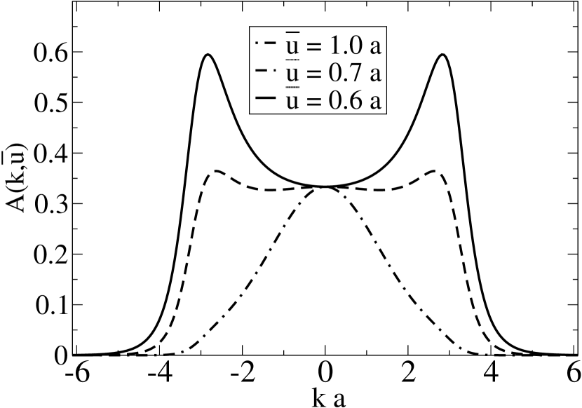
Figure 12: Spectral function $A(k,\bar{u})$, which determines the momentum dependence of tunneling in the free-spin regime. The quantity $\bar{u}$ is the root-mean-square electron displacement, due to quantum fluctuations, from the sites of a classical Wigner crystal, and $a$ is the lattice spacing. When $\bar{u}\gtrsim a$, the momentum distribution is single lobed and peaked about zero momentum. In the opposite limit, when $\bar{u}\ll a$, the momentum distribution exhibits a doubled lobed structure with peaks near $k=\pm\tilde{k}_{F}=\pm\pi/a$. The peaks have width slightly less than $\tilde{k}_{F}$, in agreement with Eq. (60) obtained from the Green’s function (51).

One can also obtain the double-lobed structure of ${\cal G}(k,\tau)$ in the limit where $\bar{u}\ll a$ by Fourier transforming Eq. (51), although it is, strictly speaking, only a valid approximation when $z\gg a$, while it is the region $z\sim a$ which dominates the spectral properties. Neglecting the slowly-varying phases $\varphi_{g}^{\pm}$, Eq. (51) gives ${\cal G}(k,\tau)\approx\mathcal{A}_{+}+\mathcal{A}_{-}$, with

$$\mathcal{A}_{\pm}(k)\propto\frac{1}{(k\pm\tilde{k}_{F})^{2}+(\tilde{k}_{F}\frac{\ln 2}{\pi})^{2}}\;.$$ (60)

The density of states for tunneling into a single point $x$, far from the ends of the wire, at a finite energy $\omega$, is approximately given by $\mathcal{A}(\omega)\approx\tau\mathcal{G}(z=0,\tau)$, with $\tau=\omega^{-1}$. Using (54), we see that when $\bar{u}$ is of order $a$ or larger, the frequency-dependence of the tunneling density of states is given by $\mathcal{A}(\omega)\propto\omega^{\tilde{\alpha}}/\bar{u}$, withFiete and Balents (2004)

$${\tilde{\alpha}}=\frac{1}{4g}-1.$$ (61)

This implies that for $4g>1$ the density of states diverges as $\omega$ decreases, unlike the behavior of a Luttinger Liquid, while for $4g<1$ the tunneling density of states is suppressed, qualitatively similar to the behavior of a Luttinger Liquid.exp

The density of states must be modified if one tunnels into a point near to the end of a semi-infinite wire, so that the distance from the end is small compared to $v_{c}/\omega$. For $\tau>x/v_{c}$, the expectation values $\langle\Theta^{2}\rangle$, $\langle\Phi^{2}\rangle$, and $\langle\Phi\Theta\rangle$, which enter (54) are affected by the proximity of the boundary. In particular, fluctuations in $\Theta$ are reduced, but $\langle\Phi^{2}\rangle$ is doubled near the end of the wire, leading to a reduction of the tunneling amplitude. One finds, for fixed value of $x$ and $\omega\to 0$, that the tunneling density of states scales as $\mathcal{A}(x,\omega)\propto\omega^{{\tilde{\alpha}}_{\rm{end}}}x^{{\tilde{\alpha}}_{\rm{end}}-{\tilde{\alpha}}}$ , where

$${\tilde{\alpha}}_{\rm{end}}=\frac{1}{2g}-1.$$ (62)

We now discuss in greater detail the effects of finite system length $L$. To obtain the resonant tunneling amplitude in the free-spin regime, we need to calculate the function

$$\mathcal{G}(x,x^{\prime})=[\,\sum_{\alpha\sigma}\langle\beta|\psi_{\sigma}(x)|\alpha\rangle\langle\alpha|\psi_{\sigma}^{\dagger}(x^{\prime})|\beta\rangle\,]_{\rm{ave}}.$$ (63)

Here, $\alpha$ and $\beta$ denote the spin states of the system with $N$ and $N-1$ electrons, respectively, and the average is taken over the spin states $\beta$. The tunneling conductance (1) is given by [see Eq. (5)]

$$G_{\pm}\sim\lambda^{2}\beta\nu\int\,dx\,dx^{\prime}e^{-ik_{\pm}(x-x^{\prime})}\mathcal{G}(x,x^{\prime})\;.$$ (64)

The function $\mathcal{G}(x,x^{\prime})$ is determined by the function $\mathcal{G}(x,x^{\prime},\tau)$, in the limit $\tau\to\infty$, which we can evaluate using the same steps as in Eq. (54) above. Because of the exponential dependence of the first factor in Eq. (47), we are only concerned with situations with $|x-x^{\prime}|\ll L$. We must now take into account the discreteness of the normal modes, as well as the proximity of the boundary, with the result that the expectation values $\langle\Theta^{2}\rangle$ and $\langle\Phi^{2}\rangle$, entering (54), depend on $x/L$, as well as, logarithmically, on $L/a$. The general result is

$$\mathcal{G}(x,x^{\prime})\sim\frac{L^{-1}(a/L)^{\tilde{\alpha}}}{\sqrt{g\ln(L/a)}}\left[\sin\left(\frac{\pi x}{L}\right)\right]^{{\tilde{\alpha}}_{\rm{end}}-{\tilde{\alpha}}}f(x-x^{\prime}),$$ (65)

where ${\tilde{\alpha}}$ and ${\tilde{\alpha}}_{\rm{end}}$ are given by (61) and (62), and $f(x-x^{\prime})$ is given by (55) with $\bar{u}=\bar{u}(L/v_{c})$ . (The derivation of these results is similar to that used in Ref. [Kane et al., 1997] to discuss tunneling into a finite carbon nanotube.)

The amplitude for momentum-resolved tunneling is determined by the Fourier transform of (65) with respect to the difference variable $(x-x^{\prime})$. Thus we recover the $k$-dependence $A(k,\bar{u})$, given by (58) with $\bar{u}=\bar{u}(L/v_{c})$.

We see that in the limit of large $N$ there are two qualitatively different features to be expected in the tunneling between parallel quantum wires in the free-spin (spin incoherent) regime compared to the ground state (spin coherent) tunneling regime: (1) The momentum structure is no longer sharply peaked at $k=\pm k_{F}$ at zero bias with the peaks splitting at the spin/charge velocity slopes at a finite bias, but depends on the relative size of $\bar{u}$ and the mean electron spacing $a$. When $\bar{u}\gg a$, the momentum distribution has a single broad peak centered at $k=0$, while when $\bar{u}\ll a$, the momentum distribution has a double lobed structure peaked at $k=\pm\tilde{k}_{F}$ at zero bias with the peak position shifting at the charge-velocity slope at a finite bias. Note, also, that $\tilde{k}_{F}$ is twice as large as $k_{F}$ for unpolarized electrons at the same density. (2) Depending on the interaction parameter $g$ of the charge sector, it is possible to have a diverging tunneling density of states as the energy is lowered. This behavior contrasts with the ubiquitous power law suppression of the spin-coherent Luttinger Liquid regime.

VI.4 Effects of non-zero Zeeman field

Our results for the free-spin regime can be generalized to the situation where the Zeeman energy $E_{Z}=g_{s}\mu_{B}B$ is comparable to $k_{B}T$, but large compared to the exchange energy $J$. In this case the spins will be partially polarized, but uncorrelated, and we can use essentially the same analysis as before. The primary modification is that the probability $p_{m}$ for $|m|+1$ consecutive spins that are all spin up or all spin down, respectively, which appears in Eq. (41), is now given by

$$p_{m}=w_{+}^{|m|+1}+w_{-}^{|m|+1}\;,$$ (66)

where $w_{+}=1-w_{-}=(1+e^{-E_{Z}/k_{B}T})^{-1}$ is the probability for finding a spin aligned parallel to the field.

To implement this change, the factors $2^{-|j|}$ in (54) and (55) must be replaced by $p_{j}$ . The function $A(k,\bar{u})$, which describes the momentum dependence of the tunneling rate, is now given by

$$A(k,\bar{u})=e^{-k^{2}\bar{u}^{2}/2}(F_{+}+F_{-})\;,$$ (67)

$$F_{\pm}\equiv\frac{w_{\pm}(1-w_{\pm}^{2})}{1+w_{\pm}^{2}+2w_{\pm}\cos(ka)}\;.$$ (68)

It may be readily seen that when the degree of polarization is increased, the peaks of $A(k,\bar{u})$ at $k=\pm{\tilde{k}}_{F}$ become higher and narrower, while the weight decreases elsewhere.(The higher momentum peaks are exponentially supressed by the prefactor in Eq. (67).) If $ka$ is fixed at any value other than an odd multiple of $\pi$, then the value of $A(k,\bar{u})$ will vanish in the limit $w_{+}\to 1$. By contrast, if $ka$ is equal to an odd multiple of $\pi$, the value of $A(k,\bar{u})$ will diverge in this limit, proportional to $w_{-}^{-1}$. The function $A(k,\bar{u})$ is plotted in Fig. 13 for several values of $x=E_{Z}/k_{B}T$ with $\bar{u}=0.6a$. Compare with Fig. 12.

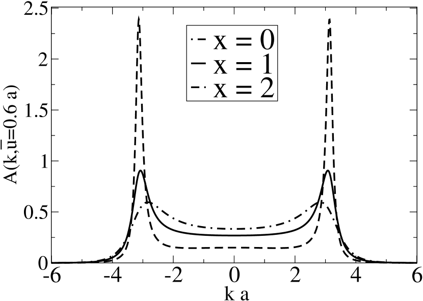
Figure 13: Polarization dependence of the spectral function given by Eqs. (67) and (68). Here $x=E_{Z}/k_{B}T$ with $E_{Z}$ the Zeeman energy and $T$ the temperature. We have used $\bar{u}=0.6a$ for each curve. (See Fig. 12 for the dependence on $\bar{u}$ at $E_{Z}=0$.) As the polarization increases, the peaks at $\tilde{k}_{F}=\pi/a$ become narrower and higher as described in the text and the weight between the peaks decreases.

To estimate the amplitude for resonant tunneling into a single point near the center of the wire, we can use (65), with $x=x^{\prime}=L/2$ . The function $f$ is to be evaluated using (55), with the factor $2^{-|j|}$ replaced by $p_{j}$, and $\bar{u}$ given by (59) . For any value of the polarization less than unity, the value of $f(z=0,\bar{u})$ is finite in the limit $\bar{u}\to\infty$, so we find

$$\mathcal{G}(x,x)\sim L^{-(1+\tilde{\alpha})}\ln^{-1/2}(L/a)\;,$$ (69)

for $L\to\infty$ with ${\tilde{\alpha}}$ given by (61). On the other hand, for a fully polarized system, with $w_{+}=1$, one finds that $f(z=0,\bar{u})$ vanishes like $\bar{u}L^{-g}$ for $L\to\infty$ and $\bar{u}$ given by (59). One then finds

$$\mathcal{G}(x,x)\sim 1/L^{(1+\alpha_{p})}\;,$$ (70)

with $\alpha_{p}=g+(4g)^{-1}-1$ . This exponent is the same as the standard tunneling exponent one would obtain for spinless fermions having the same interaction and density, if one takes into account the difference in the definitions of $g$ for the two cases. (Here, we have defined $g$ as $v_{F}/v_{c}$, where $v_{F}$, the Fermi velocity for non-interacting spinless fermions, is half of the Fermi velocity for spinless fermions at the same density.)

VII Comparison with experiments

Results for the momentum-dependence of the tunneling conductance, obtained in the present paper, show various similarities and differences with the experimental results of Steinberg et al.Ste ; Auslaender et al. (2005) in the localized regime (that is, the regime in which the tunneling exhibits broad structure in momentum space and hence local structure in position space). In general, experimental results at the first Coulomb blockade peak, associated with the first electron to tunnel into the localized region, show a single peak, centered at $k=0$, as expected from our analysis. However, the spectrum for the second and subsequent electrons typically show two peaks, at positions $\approx\pm k_{m}$ that increase with increasing $N$. The intensity between the two peaks is not small, being perhaps half the intensity at the maxima, and one does not observe the zeroes of the intensity that we find for ground-state tunneling in a symmetric well.

Qualitatively, the experiments are most consistent with our results for the free-spin regime, i.e., the results one would expect when $k_{B}T$ is large compared to $J$ but small compared to the energy for charge excitations. According to the results of Subsection V.5 above, $J$ should indeed be smaller than the experimental temperature of 0.25 K, for densities less than about 6 electrons per $\mu$m. The confinement length $L$ in the experiments is not precisely known, and it may well change as additional electrons are added, but if one estimates $L$ in the range of 0.5 to 1 $\mu$m, the free-spin regime would hold for values of $N$ less than perhaps 3 to 6. On the other hand, there is evidence that for the largest values of $N$ in the localized regime, the density reaches 15 electrons per $\mu$m, for which we estimate a value of $J$ much larger than $k_{B}T$.

An added factor in the experiments is that the Zeeman energy is not negligible compared to $k_{B}T$. For a typical applied field of 2 T, the Zeeman energy is about 0.6 K, more than twice the quoted temperature. If the Zeeman energy is comparable to, but smaller than $J$, the system will be partially polarized even at $T=0$. For $J\sim E_{Z}>k_{B}T>J/N$, typically a number of different spin states will be occupied. Theoretical expectations for the case with a sizable Zeeman energy were discussed briefly in Subsection VI.4 above, for the free spin regime, and they may be qualitatively consistent with the experiments.

We recall that in the free-spin regime (provided that $\bar{u}<0.75a$), or in the fully-polarized regime, the position of the intensity maximum should occur at $k_{m}\approx 2k_{F}$, where $k_{F}$ is the Fermi wavevector for unpolarized electrons at the same density. There is no experimental indication of this when the upper wire is in the delocalized (that is, the Luttinger Liquid regime) regime. Thus if the electrons in the localized regime (see first paragraph of this section above) form either a free-spin or a spin-polarized lattice, there should be an increase in the value of $k_{m}$ as one enters the localized regime. It is not clear whether such an effect is observed in the experiments. The tendency for an increase in $k_{m}$ may be counteracted if there is a discontinuous decrease in electron density upon entering the localized regime.

The situation where $k_{B}T$ and $E_{Z}$ are both large compared to $J$ was discussed for the simplest case, $N=2$, in Subsection V.6, and illustrated in Fig. 10. Under the experimental conditions where $E_{Z}$ is large compared to $k_{B}T$, the momentum dependence of the conductivity should be close to that of the pure triplet state, and should have near zero intensity at $k=0$, if the confining well is symmetric. This contrasts with the experimental data for $N=2$, where the intensity at $k=0$ is a substantial fraction of the maximum intensity. The discrepancy might be explained if the confining well is sufficiently asymmetric, or if the electron temperature in the upper wire is significantly higher than the lattice temperature.

The calculations in Section V above used a model with sharp confinement at the ends of the wire and a flat potential within. We presented exact numerical diagonalizations for two and four electrons. A model with soft confinement, and higher density near the center of the wire, would lead to more intensity at $|k|<k_{m}$, and a faster fall-off of intensity for $|k|>k_{m}$, than one obtains in the case of sharp confinement.Tserkovnyak et al. (2002, 2003)

Finally, we repeat that the reason for the apparent formation of a barrier between the low-density central section of the upper wire and the high density outer regions is not well understood.

VIII Conclusions

In this paper we have studied momentum resolved tunneling into a short quantum wire. We have focused on the situation where the number of electrons, $N$, is not too large and the density of electrons is low enough to approach the Wigner crystal limit. We began by reviewing some general theorems which dictate basic properties of the momentum dependence. We note that the matrix element for tunneling between ground states for $N$ and $N-1$ electrons can be expressed in terms of the Fourier transform of a real function $\Psi_{\rm{eff}}(x)$, which is the matrix element of $\psi_{\sigma}(x)$, the electron annihilation operator at point $x$, between the two states. For non-interacting electrons, $\Psi_{\rm{eff}}(x)$, is the wavefunction of the highest filled level in the $N$-electron system; more generally, $\Psi_{\rm{eff}}(x)$ is a quasi-wavefunction, whose magnitude is reduced by many-body correlations, but whose spatial dependence is qualitatively similar to the non-interacting case.

Using exact diagonalization, we computed the ground-state density, the density-density correlation function, and the effective exchange constant, $J$, for $N\leq 4$. We include screening effects from the adjacent, higher density wire. In the limit of large $N$ we applied bosonization techniques to study the momentum resolved tunneling, both at $T=0$, and in the free-spin limit, of spin energies much less than temperature and the Fermi energy, $J\ll k_{B}T\ll E_{F}$. Whereas for $k_{B}T\ll J,E_{F}$, the momentum dependence has narrow peaks centered at $k=\pm k_{F}$, in the free-spin regime, the spectral function can have broad peaks centered at $k=\pm 2k_{F}$. Comparisons of our theoretical predictions with experimental results obtained by Steinberg et al.Ste ; Auslaender et al. (2005) show qualitative agreement on many features, but some aspects are still not understood, and further work is needed.

While we were finishing this manuscript, we became aware of independent unpublished work by E. J. Mueller, based on the experiments that motivated our study.Mue Mueller’s work employs, primarily, a Hartree-Fock approximation, and is largely orthogonal to the work reported here.