Effects of Diversity on Multi-agent Systems:
Minority Games

Abstract

We consider a version of large population games whose agents compete for resources using strategies with adaptable preferences. The games can be used to model economic markets, ecosystems or distributed control. Diversity of initial preferences of strategies is introduced by randomly assigning biases to the strategies of different agents. We find that diversity among the agents reduces their maladaptive behavior. We find interesting scaling relations with diversity for the variance and other parameters such as the convergence time, the fraction of fickle agents, and the variance of wealth, illustrating their dynamical origin. When diversity increases, the scaling dynamics is modified by kinetic sampling and waiting effects. Analyses yield excellent agreement with simulations.

I Introduction

Many natural and artificial systems involve interacting agents, each making independent decisions to compete for limited resources, but globally exhibit coordinated behavior through their mutual adaptation Anderson et al. (1988); Weiß and Sen (1995); Schweitzer (2002); Challet and Zhang (1997). Examples include the formation of ecological patterns due to the competition of predators hunting for food, the price adjustment due to the competition of buyers or sellers in economic markets, and the load adjustment due to the competition of distributed controllers of packet flows in computer networks. While a standard approach is to analyse the steady state behavior of the system described by the Nash equilibria Rasmusen (1989), it is legitimate to consider how the steady state is approached, since such processes are dynamical in nature, and the approach may be interfered by the presence of periodic, chaotic or metastable attractors. Dynamical studies are especially relevant when one considers the effects of changing environment, such as that in economics or distributed control.

The recently proposed Minority Games (MG) are prototypes of such multi-agent systems Challet and Zhang (1997). Extensive studies have revealed the steady-state properties of the game when the complexity of the agents is high Challet et al. (2000). On the other hand, the dynamical nature of the adaptive processes is revealed when the complexity of the agents is low, wherein the final states of the system depend on the initial conditions, and the system often ends up with large fluctuations at final states, much remote from the efficient state predicted by equilibrium studies Challet et al. (2000); Garrahan et al. (2000). The large fluctuations in the original MG is related to the uniformly zero preference of strategies for all agents. This has to be re-examined for at least two reasons. First, when the game is used to model economic systems, it is not realistic to expect that all agents have the same preference when they enter the market. Rather, the agents have their own preferences according to their individual objectives, expectations and available capital. For example, some have stronger inclinations towards aggressive strategies, and others more conservative. Furthermore, in games which use public information only, identical initial preferences imply that different agents would maintain identical preferences of strategies at all subsequent steps of the game, which is again unlikely. Second, when the game is used to model distributed control in multi-agent systems, identical preferences of strategies of the agents lead to maladaptive behavior, which refers to the bursts of the population’s decisions due to the agents’ premature rush to certain state Savit et al. (1999); Johnson et al. (1999a). As a result, the population difference between the majority and minority groups is large. For economic markets, this corresponds to large price fluctuations; for distributed control, this corresponds to an uneven resource allocation; both imply low system efficiency. Hence, maladaptation hinders the attainment of optimal system efficiency.

There have been many attempts to improve the system efficiency. For example, thermal noise Cavagna et al. (1999) or biased strategies Yip et al. (2003) are found to reduce the fluctuations. More relevant to this work, there were indications that maladaptation can be reduced by appropriate choices of the initial condition at the low complexity phase. The dependence of initial conditions was noted in the replica approach to the exogenous MG Challet et al. (2000). System efficiency can be improved by random initial conditions in the original MG Moro (2004), or systems driven by vectorized external information Garrahan et al. (2000). It was noted that the reduced variance can be obtained hysteretically by quasistatic increase and decrease of the complexity from an unbiased initial condition, clearly demonstrating the non-equilibrium nature of this phenomenon Sherrington et al. (2002a). By generalizing the strategy evaluation mechanism to the batch mode, and using a payoff function linear in the winning margin, the generating functional analysis showed that fluctuations are reduced by biased starts of the agents’ strategy payoff valuations Heimel and Coolen (2001). The same is valid in its noisy extension Coolen et al. (2001). However, no systematic studies about the effects of random biases have been made.

In this paper, we consider the effects of randomness in the initial preferences of strategies among the agents. Initial conditions can be selected to make the system dynamics completely deterministic, thus yielding highly precise simulation results useful for refined comparison with theories. As we shall see, a consequence of this diversity is that agents sharing common strategies are less likely to adopt them at the same time, and maladaptation is reduced. This results in an improved system efficiency, as reflected by the reduced variance of the population decisions. We find interesting scaling relations with the diversity for the variance, and a number of dynamical parameters, such as the convergence time, the fraction of fickle agents, and the variance of wealth, illustrating their dynamical origin. When diversity increases, we find that the scaling dynamics is modified by a sampling mechanism self-imposed by the requirement of the dynamics to stay in the attractor, an effect we term kinetic sampling. Preliminary results have been sketched in Wong et al. (2004).

This paper is organized as follows. After introducing the Minority Game in Section II, we discuss the variation of fluctuations when diversity increases, identifying 3 regimes of behavior: multinomial, scaling, and kinetic sampling, analyzed in Sections III to V respectively. Besides the fluctuations, other dynamical properties, namely, the fraction of fickle agents, the convergence time, and the variance of wealth, are discussed in Sections VI to VIII respectively. The paper is concluded in Section IX.

II The Minority Game

We consider a population of $N$ agents competing selfishly to be in the minority group in an environment of limited resources, $N$ being odd Challet and Zhang (1997). Each of the $N$ agents can make a decision 1 or 0 at each time step, and the minority group wins. For typical control tasks such as the distribution of shared resources, the decisions 1 and 0 may represent two atternative resources, so that less agents utilizing a resource implies more abundance. For economic markets, the decisions 1 and 0 correspond to buying and selling respectively, so that the buyers can win by belonging to the minority group, as a consequence of the price being pushed down when supply is greater than demand, and vice versa.

Each agent makes her decision independently according to her own finite set of strategies, randomly picked before the game starts. Each of her $s$ strategies is based on the history of the game, which is the time series of the winning bits in the most recent $m$ steps. Hence, $m$ is the memory size. There are $D\equiv 2^{m}$ possible histories, thus $D$ is the dimension of the strategy space. While most previous work considered the case $D\sim N$, we will mainly study the case $m\gtrsim 1$ in this paper. As we shall see, this simplification enables us to make detailed analysis of the system, revealing many new features.

A strategy is then a Boolean function which maps each of the $D$ histories to decisions 1 or 0. Denoting the winning state at time $t$ by $\sigma(t)$ ($\sigma(t)=1,0$), we can convert an $m$-bit history $\sigma(t-m+1),\cdots,\sigma(t)$ to an integer historical state $\mu^{*}(t)$ of modulo $D$, given by

$$\mu^{*}(t)=\sum_{t^{\prime}=0}^{m-1}\sigma(t-t^{\prime})2^{t^{\prime}},$$ (1)

and the Boolean decisions of strategy $a$ responding to input state $\mu$ are denoted by $\sigma_{a}^{\mu}=1,0$, corresponding to the binary decisions $\xi_{a}^{\mu}=\pm 1$ via $\xi_{a}^{\mu}\equiv 2\sigma_{a}^{\mu}-1$. For subsequent analyses of strategies, the label $a$ of a strategy is given by an integer between 0 and $2^{D}-1$, where

$$a=\sum_{\mu=0}^{D-1}\sigma_{a}^{\mu}2^{D-1-\mu}.$$ (2)

The success of a strategy is measured by its cumulative payoff (also called virtual point in the literature), which increases (decreases) by $1$ if it indicates a winning (losing) decision at a time step. Note that the payoffs attributed to the strategies at each step depend only on the signs of the decisions, and is independent of the magnitude of the winning margins. This is called the step payoff, and follows the original version of the MG Challet and Zhang (1997). Many recent studies used payoffs with magnitudes increasing with the difference between the majority and minority population. In particular, payoffs that are linear in the population difference are called linear payoffs, and are found convenient in the application of analytical techniques such as the replica method Challet et al. (2000) or the generating functional analysis Heimel and Coolen (2001). In the analysis of this paper, the step payoff is more convenient.

At each time step, each agent chooses, out of her $s$ strategies, the one with the highest cumulative payoff (updated every step irrespective of whether it is adopted or not) and makes decisions accordingly. The difference between the total number of winning and losing decisions of an agent up to a time step is called her wealth at that time. The long-term goal of an agent is to maximize her wealth.

To model diversity among the agents, the agents may enter the game with diverse preferences of their strategies. This means that each agent has random integer biases to the initial cumulative payoffs of each of her $s$ strategies. We are interested in how the extent of randomness affects the system behavior, and there are many choices of the bias distribution. A natural choice is the multinomial distribution, which can be modeled by assigning integer biases to the $s$ strategies of each agent, which add up to an odd integer $R$. Then, the biased payoff of a strategy of an agent obeys a multinomial distribution with mean $R/s$ and variance $R(s-1)/s^{2}$. The ratio $\rho\equiv R/N$ is referred to as the diversity.

For the binomial case $s=2$ and odd $R$, which will be studied here, no two strategies have the same cumulative payoffs throughout the game. Hence there are no ties, and the dynamics of the game is deterministic, resulting in highly precise simulation results useful for refined comparison with theories. This is in contrast with previous versions of the game, which correspond to the special case of $R=0$.

Furthermore, for an agent holding strategies $a$ and $b$ (with $a<b$), the biases affect her decisions only through the bias difference $\omega$ of strategy $a$ with respect to $b$. Hence we let $S_{ab}(\omega)$ be the number of agents holding strategies $a$ and $b$, where the bias of strategy $a$ is displaced by $\omega$ with respect to $b$, and its disordered average is

$$\langle S_{ab}(\omega)\rangle=\frac{N}{2^{2D-1}}\frac{1}{2^{R}}\binom{R}{\frac{R-\omega}{2}}.$$ (3)

To describe the macroscopic dynamics of the system, we define the $D$-dimensional phase space with the components $A^{\mu}(t)$, which is the fraction of agents making decision 1 responding to input $\mu$ of their used strategies, subtracted by that for decision $0$. While only one of the $D$ components corresponds to the historical state $\mu^{*}(t)$ of the system, the augmentation to $D$ components is necessary to describe the attractor structure and the transient behavior of the system dynamics.

The key to analysing the system dynamics is the observation that the cumulative payoffs of all strategies displace by exactly the same amount when the game proceeds, though their initial values may be different. Hence for a given strategy pair, the profile of the cumulative payoff distribution remains binomial, but the peak position shifts with the game dynamics. Hence once the cumulative payoffs are known, the state location in the $D$-dimensional phase space is given by

$$A^{\mu}(t) = \frac{1}{N}\sum_{a<b,\omega}S_{ab}(\omega)\left\{\Theta[\omega+\Omega_{a}(t)-\Omega_{b}(t)]\xi_{a}^{\mu}+\Theta[-\omega-\Omega_{a}(t)+\Omega_{b}(t)]\xi_{b}^{\mu}\right\}$$ (4)

$$+\frac{1}{N}\sum_{a}S_{a}\xi_{a}^{\mu},$$

where $\Omega_{a}(t)$ is the cumulative payoff of strategy $a$ at time $t$, $S_{a}$ is the number of agents holding 2 identical strategies labelled $a$, and $\Theta(x)$ is the step function of $x$. For agents holding non-identical strategies $a<b$, the agents make decision according to strategy $a$ if $\omega+\Omega_{a}(t)-\Omega_{b}(t)>0$, and strategy $b$ otherwise. Hence $\omega+\Omega_{a}(t)-\Omega_{b}(t)$ is referred to as the preference of $a$ with respect to $b$. In turn, the cumulative payoff of a strategy $a$ is updated by

$$\Omega_{a}(t+1)=\Omega_{a}(t)-\xi_{a}^{\mu^{*}(t)}{\rm sgn}A^{\mu^{*}(t)}(t).$$ (5)

Fig. 1(a) illustrates the convergence to the attractor for the visualizable case of $m=1$. The dynamics proceeds in the direction which tends to reduce the magnitude of the components of $A^{\mu}(t)$ Challet et al. (2000). However, a certain amount of maladaptation always exists in the system, so that the components of $A^{\mu}(t)$ overshoot, resulting in periodic attractors of period $2D$, as reported in the literature Zheng and Wang ; Lee (2001). The state evolution is given by the integer equation

$$\mu^{*}(t+1)={\rm mod}(2\mu^{*}(t)+\sigma(t),D),$$ (6)

so that every state $\mu$ appears as historical states two times in a steady-state period, with $\sigma(t)$ appearing as 0 and 1, each exactly once. One occurence brings $A^{\mu}$ from positive to negative, and another bringing it back from negative to positive, thus completing a cycle. The components keep on oscillating, but never reach zero. This results in an antipersistent time series Metzler (2002). For the example in Fig. 1(a), the steady state is described by the sequence

$$\mu(t)=\sigma(t)=0,1,1,0,$$ (7)

where one notes that both states 0 and 1 are followed by 0 and 1 once each.

For $m=2$, there are 2 attractor sequences as shown in Fig. 1(b),

$$\mu(t)=0,1,3,3,2,1,2,0,$$ (8)

and

$$\mu(t)=0,1,2,1,3,3,2,0.$$ (9)

Again, one notes that each of the states 0, 1, 2, 3 are followed by an even ($\sigma(t)=0$) and an odd state ($\sigma(t)=1$) once each. Furthermore, we note that the attractor sequences in Eqs. (8) and (9) are related by the conjugation symmetry $\mu(t)\rightarrow 3-\mu(t)$. For general values of $m$, an attractor sequence can be obtained by starting with the state $\mu^{*}(0)=\sigma(0)=0$, and assigning $\sigma(t)=1$ if the value of $\mu^{*}(t)$ appears the first time in the sequence, and 0 the second time, such as the attracters in Eq. (7) and (8). In general, other attractor sequences can be obtained by computer search, and the number of attractor sequences can be verified to be $2^{D}/2D$, which forms the de Bruijn sequence in terms of $m$, corresponding to the number of distinct ring configurations of length $2D$, for which all sub-strings of length $m+1$ are distinct Golomb (1982).

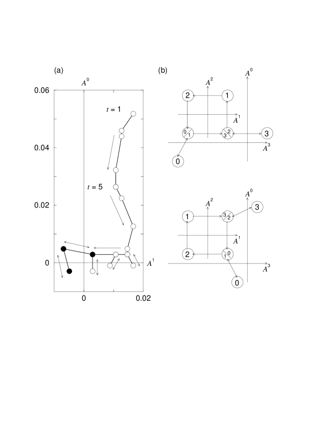
Figure 1: (a) The state motion of a sample in the phase space for $m=1$, $s=2$, $N=1023$ and $R=16383$. Empty dots: transient states. Solid dots: attractor states. (b) The attractors in the phase subspace of $A^{1}$ and $A^{2}$ for $m=2$. 6 of the 8 states remain in the second quadrant of the subspace formed by $A^{3}$ and $A^{0}$. The location of the other 2 states are indicated in the $A^{3}$ and $A^{0}$ subspace, instead of the $A^{1}$ and $A^{2}$ subspace. The numbers in the circles denote the elements of the attractor sequences in Eqs. (8) and (9).

The population averages of the decisions oscillate around 0 at the steady state. Since a large difference between the majority and minority populations implies inefficient resource allocation, the inefficiency of the game is often characterized by the normalized variance $\sigma^{2}/N$ of the population making decision 1 at the steady state. Since this population size at time $t$ is given by $N(1-A^{\mu^{*}(t)})/2$, we have

$$\frac{\sigma^{2}}{N}=\lim_{t\rightarrow\infty}\frac{N}{4}\langle[A^{\mu^{*}}(t)-\langle A^{\mu^{*}}(t)\rangle_{t}]^{2}\rangle_{t},$$ (10)

where $\langle\quad\rangle_{t}$ denotes time average at the steady state.

Figure 2: The dependence of the variance of the population making decision $+$ on the complexity for different diversities at $s=2$ averaged over 128 samples. The horizontal dotted line is the limit of random decisions.

As shown in Fig. 2, the variance $\sigma^{2}/N$ of the population for decision 1 scales as a function of the complexity $\alpha\equiv D/N$, agreeing with previous observations Savit et al. (1999). When $\alpha$ is small, games with increasing complexity create time series of decreasing fluctuations. A phase transition takes place around $\alpha_{c}\approx 0.3$, after which it increases gradually to the limit of random decisions, with $\sigma^{2}/N=0.25$. When $\alpha<\alpha_{c}$, the occurences of decision 1 and 0 responding to a given historical state $\mu$ are equal, and is referred to as the symmetric phase Challet and Marsili (1999). On the other hand, in the asymmetric phase above $\alpha_{c}$, the occurences of decisions are biased for at least some history $\mu$.

Figure 2 also shows the data collapse of the variance for different values of diversity $\rho$. It is observed that the variance decreases significantly with diversity in the symmetric phase, and remains unaffected in the asymmetric phase com (a). Furthermore, for a game efficiency prescribed by a given variance $\sigma^{2}/N$, the required complexity of the agents is much reduced.

The dependence of the variance on the diversity is further shown in Figs. 3 and 4 for memory sizes $m=1$ and $m=2$ respectively. The following three regimes can be identified and explained in Sections III to V respectively: (a) multinomial regime: when $\rho\sim N^{-1}$, $\sigma^{2}/N\sim N$ with proportionality constants dependent on $m$; (b) scaling regime: when $\rho\sim 1$, $\sigma^{2}/N\sim\rho^{-1}$ with proportionality constants independent of $m$ for $m$ not too large; (c) kinetic sampling regime: when $\rho\sim N$, $\sigma^{2}/N$ deviates above the scaling with $\rho^{-1}$ due to kinetic sampling effects as explained below, and the scaling is given by $\sigma^{2}/N\sim f_{m}(\Delta)/N$, where $\Delta$ is the kinetic step size given by

$$\Delta\equiv N\sqrt{\frac{2}{\pi R}}=\sqrt{\frac{2N}{\pi\rho}},$$ (11)

and $f_{m}$ is a function dependent on the memory size $m$.

Figure 3: The dependence of the variance of the population making decision $+$ on the diversity at $m=1$ and $s=2$. Symbols: simulation results averaged over 1024 samples. Solid lines: theory. Dashed-dotted line: scaling prediction.

Figure 4: The dependence of the variance of the population making decision $+$ on the diversity at $m=2$ and $s=2$. Notations are the same as those of Fig. 3. Inset: A comparison of the variances at $m=1$ and $m=2$ in Figs. 3 and 4.

To analyse the behavior in these regimes, we derive the following expression for the step $\Delta A^{\mu}(t)\equiv A^{\mu}(t+1)-A^{\mu}(t)$, at time $t$. Using Eq. (4), we have

$$\Delta A^{\mu}(t)=\frac{1}{N}\sum_{a<b,\omega}S_{ab}(\omega)\{\Theta[\omega+\Omega_{a}(t+1)-\Omega_{b}(t+1)]-\Theta[\omega+\Omega_{a}(t)-\Omega_{b}(t)]\}(\xi_{a}^{\mu}-\xi_{b}^{\mu}).$$ (12)

Since the arguments of the step functions are odd integers, nonzero contributions to Eq. (12) come from terms with $\omega+\Omega_{a}(t+1)-\Omega_{b}(t+1)=\pm 1$ and $\omega+\Omega_{a}(t)-\Omega_{b}(t)=\mp 1$. Using Eq. (5), the two arguments differ by $-(\xi_{a}^{\mu}-\xi_{b}^{\mu}){\rm sgn}A^{\mu}(t)$ with $\mu=\mu^{*}(t)$. Hence the conditions for nonzero contributions become equivalent to $\omega+\Omega_{a}(t)-\Omega_{b}(t)=\mp 1$ and $\xi_{a}^{\mu}-\xi_{b}^{\mu}=\mp 2{\rm sgn}A^{\mu}(t)$ for $\mu=\mu^{*}(t)$. This reduces the steps to

$$\Delta A^{\mu}(t)=\frac{1}{N}\sum_{a<b,\omega,\pm}S_{ab}(\omega)\delta(\omega+\Omega_{a}(t)-\Omega_{b}(t)\pm 1)\delta(\xi_{a}^{\mu}-\xi_{b}^{\mu}\pm 2{\rm sgn}A^{\mu}(t))(\pm)(\xi_{a}^{\mu}-\xi_{b}^{\mu}),$$ (13)

where $\mu=\mu^{*}(t)$, and $\delta(n)=1$ if $n=0$, and 0 otherwise. For $\mu=\mu^{*}(t)$, this can be further simplified to

$$\Delta A^{\mu}(t)=-{\rm sgn}A^{\mu}(t)\frac{2}{N}\sum_{a<b,\pm}S_{ab}(\mp 1-\Omega_{a}(t)+\Omega_{b}(t))\delta(\xi_{a}^{\mu}-\xi_{b}^{\mu}\pm 2{\rm sgn}A^{\mu}(t)),$$ (14)

To interpret this result, we note that changes in $A^{\mu}(t)$ are only contributed by fickle agents with marginal preferences of their strategies. That is, those with $\omega+\Omega_{\alpha}(t)-\Omega_{\beta}(t)=\pm 1$ and $\xi_{\alpha}^{\mu}-\xi_{\beta}^{\mu}=\mp 2{\rm sgn}A^{\mu}(t)$ for $\mu=\mu^{*}(t)$. Furthermore, the step points in the direction that reduces the magnitude of $A^{\mu}(t)$.

Similarly, the steps along the direction $\nu$ other than the historical state $\mu^{*}(t)$ are given by

$$\Delta A^{\nu}(t)=\frac{1}{N}\sum_{a<b,\pm}S_{ab}(\mp 1-\Omega_{a}(t)+\Omega_{b}(t))\delta(\xi_{a}^{\mu}-\xi_{b}^{\mu}\pm 2{\rm sgn}A^{\mu}(t))(\pm)(\xi_{a}^{\nu}-\xi_{b}^{\nu})$$ (15)

where $\mu=\mu^{*}(t)$. This shows that the steps along the non-historical direction are contributed by the subset of those fickle agents that contribute to the step along the historical direction, and they can be positive or negative.

Next we consider the disordered average of the steps in Eq. (13). For this purpose, it is convenient to decompose the cumulative payoffs as

$$\Omega_{a}(t)=\sum_{\mu}k_{\mu}(t)\xi_{a}^{\mu},$$ (16)

where $k_{\mu}(t)$ is the number of wins minus losses of decision 1 up to time $t$ when the game responded to history $\mu$. Since there are $2^{D}$ variables of $\Omega_{a}(t)$ and $D$ variables of $k_{\mu}(t)$, this decomposition greatly simplifies the analysis, and describes explicity how $\Omega_{a}(t)$ depends on the strategy decisions. Introducing the integral representation of the Kronecka delta for the preference, we can factorize the contributions of $\Omega_{a}(t)-\Omega_{b}(t)$ into a product over the states,

$$\delta(\omega+\Omega_{a}(t)-\Omega_{b}(t)\pm 1)=\int_{0}^{2\pi}\frac{d\theta}{2\pi}e^{i\theta(\omega\pm 1)}\prod_{\lambda}e^{i\theta k_{\lambda}(\xi_{a}^{\lambda}-\xi_{b}^{\lambda})},$$ (17)

where the explicit dependence on $t$ is omitted for convenience here and in the subsequent derivation. Using the identities

$$\delta(\xi_{a}^{\mu}-\xi_{b}^{\mu}\pm 2{\rm sgn}A^{\mu}(t)) = \frac{1}{4}[1\mp(\xi_{a}^{\mu}-\xi_{b}^{\mu}){\rm sgn}A^{\mu}-\xi_{a}^{\mu}\xi_{b}^{\mu}],$$ (18)

$$e^{i\phi(\xi_{a}^{\mu}-\xi_{b}^{\mu})} = \cos^{2}\phi+(\xi_{a}^{\mu}-\xi_{b}^{\mu})i\sin\phi\cos\phi+\xi_{a}^{\mu}\xi_{b}^{\mu}\sin^{2}\phi,$$ (19)

and introducing the average in Eq. (3), we obtain the following factorized expression from Eq. (13) for $\mu=\mu^{*}(t)$,

$$\langle\Delta A^{\mu}(t)\rangle= \frac{1}{2^{2D-1}}\sum_{a<b,\omega,\pm}\binom{R}{\frac{R-\omega}{2}}\frac{1}{2^{R}}\int_{0}^{2\pi}\frac{d\theta}{2\pi}e^{i\theta(\omega\pm 1)}$$ (20)

$$\frac{1}{4}[1\mp(\xi_{a}^{\mu}-\xi_{b}^{\mu}){\rm sgn}A^{\mu}-\xi_{a}^{\mu}\xi_{b}^{\mu}](\pm)(\xi_{a}^{\mu}-\xi_{b}^{\mu})$$

$$[\cos^{2}k_{\mu}\theta+(\xi_{a}^{\mu}-\xi_{b}^{\mu})i\sin k_{\mu}\theta\cos k_{\mu}\theta+\xi_{a}^{\mu}\xi_{b}^{\mu}\sin^{2}k_{\mu}\theta]$$

$$\prod_{\lambda\neq\mu}[\cos^{2}k_{\lambda}\theta+(\xi_{a}^{\lambda}-\xi_{b}^{\lambda})i\sin k_{\lambda}\theta\cos k_{\lambda}\theta+\xi_{a}^{\lambda}\xi_{b}^{\lambda}\sin^{2}k_{\lambda}\theta].$$

The summation over $a<b$ can now be replaced by half times the independent summations over $a$ and $b$. Noting that for given states $\mu,\nu\ldots\lambda$,

$$\sum_{a}\xi_{a}^{\mu}\xi_{a}^{\nu}\cdots\xi_{a}^{\lambda}=0,$$ (21)

we find that all terms in the expansion of Eq. (20) vanish if they contain unpaired decisions $\xi_{a}^{\nu}$ or $\xi_{b}^{\nu}$. The final result is

$$\langle\Delta A^{\mu}(t)\rangle=-{\rm sgn}A^{\mu}\int_{0}^{2\pi}\frac{d\theta}{2\pi}\cos^{R}\theta\cos(2k_{\mu}-{\rm sgn}A^{\mu})\theta\prod_{\nu\neq\mu}\cos^{2}k_{\nu}\theta.$$ (22)

Eq. (22) describes the change induced by the payoff component $k_{\mu}(t)$ incremented by $-{\rm sgn}A^{\mu}(t)$. Since the step size depends on time implicitly through the payoff components, the sum of all changes induced by $k_{\mu}(t)$ incremented from 0 yields

$$\langle A^{\mu}(t)-A^{\mu}(0)\rangle=\int_{0}^{2\pi}\frac{d\theta}{2\pi}\cos^{R}\theta\frac{\sin k_{\mu}\theta\cos k_{\mu}\theta}{\sin\theta}\prod_{\nu\neq\mu}\cos^{2}k_{\nu}\theta.$$ (23)

Similarly, the steps along the non-historical direction are given by

$$\langle\Delta A^{\nu}(t)\rangle=\int_{0}^{2\pi}\frac{d\theta}{2\pi}\cos^{R}\theta\sin k_{\nu}\theta\cos k_{\nu}\theta\sin(2k_{\mu}{\rm sgn}A^{\mu}-1)\theta\prod_{\lambda\neq\mu\nu}\cos^{2}k_{\lambda}\theta,$$ (24)

where $\nu\neq\mu^{*}(t)=\mu$. The same result can be obtained from Eq. (23) by considering the difference of 2 equations when one of the states labeled $\nu$ become historical and $k_{\nu}$ changes by $-{\rm sgn}A^{\nu}$.

III The Multinomial Regime

When $\rho\sim N^{-1}$, or $R\sim 1$, there is a finite number of clusters of agents who make identical decisions throughout the game. Since there are many agents in a typical cluster, their identical decisions will cause large fluctuations in their behavior. Consider the example of $m=1$ and $R=1$. There are only 4 strategies. For a pair of distinct strategies, there is an average of $N/8$ agents picking them, and $N/16$ agents in each cluster with biases $\pm 1$. As a result, we have $\sigma^{2}/N\sim N$. The proportionality constant depends on $m$, and is sensitive to the profile of the bias distribution. Since we consider the multinomial distribution in Eq. (3) in this paper, we call this the multinomial regime. Another choice in the literature is the bimodal distribution Moro (2004); Garrahan et al. (2000); Sherrington et al. (2002a); Heimel and Coolen (2001); Coolen et al. (2001), which may have different behavior.

Consider the case $m=1$. Eqs. (22) and (24) show that the step size $\langle\Delta A^{\mu}(t)\rangle\sim{\cal O}(1)$ and is thus self-averaging. Since $A^{\mu}(0)$ is Gaussian with variance $N^{-1}$, the values of $A^{\mu}(t)$ at the attractors can be computed to ${\cal O}(1)$. Depending on the initial position ${\bf A}(0)\equiv(A^{1}(0),A^{0}(0))$, 4 attractors can be identified. For example, if ${\bf A}(0)$ lies in the first quadrant, and the initial historical state is 0, then the payoff components ${\bf k}\equiv(k^{1}(t),k^{0}(t))$ at the attractor are given by ${\bf k}(0)=(0,0)$, ${\bf k}(1)=(-1,0)$, ${\bf k}(2)=(-1,-1)$, ${\bf k}(3)=(-1,0)$, provided that when $\Delta A^{\mu}(t)=0$ to order 1, $\Delta A^{\mu}(t)$ is also equal to 0 to order $N^{-1/2}$. Analysis can be simplified by noting that when the payoff components $k_{\mu}(t)$ are restricted to the values 0 and $\pm 1$, Eq. (23) can be written as

$$A^{\mu}(t)=k_{\mu}\int_{0}^{2\pi}\frac{d\theta}{2\pi}(\cos\theta)^{\left[R+1+2\sum_{\nu\neq\mu}|k_{\nu}|\right]}=k_{\mu}c_{\left[R+1+2\sum_{\nu\neq\mu}|k_{\nu}|\right]},$$ (25)

where $c_{n}\equiv 2^{-n}\binom{n}{n/2}$ for even integer $n$, and we have used the facts that $A^{\mu}(t)$ is self-averaging, $A^{\mu}(0)\sim N^{-1/2}$. The locations of the 4 attractors are shown in Fig. 5 and summarised in Table 1.

The variance of $A^{\mu}(t)$ of the historical states $\mu=\mu^{*}(t)$, averaged over the period for each of the 4 attractors, can be obtained from Table 1. The variance of decisions in Eq. (10), averaged over the 4 attractors, is then given by

$$\frac{\sigma^{2}}{N}=\frac{N}{128}(7c_{R+1}^{2}-2c_{R+1}c_{R+3}+7c_{R+3}^{2}).$$ (26)

The theoretical values are compared with simulation results for the first 3 points of each curve corresponding to given values of $N$ in Fig. 3. The agreement is excellent. Note that the variance in this regime deviates from the scaling relation with $\rho^{-1}$ in the next regime, as evident from the splaying down from the linear relation in Fig. 3. However, when $R\gg 1$, $c_{R+1}\approx c_{R+3}\approx\sqrt{2/\pi R}$, $\sigma^{2}/N$ reduces to $3/16\pi\rho$, showing that the deviation from the $\rho^{-1}$ scaling gradually vanishes.

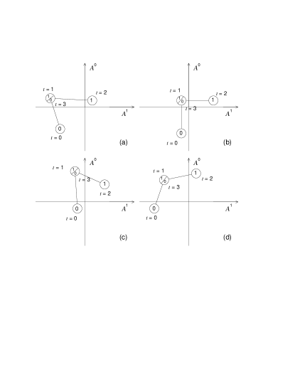
Figure 5: (a-d) The 4 attractors for $m=1$ and $s=2$ in the multinomial regime. The time steps are relabeled with $t=0$ corresponding to the state with $\mu^{*}(t)=0$ and $\mu^{*}(t+1)=1$.

$t$	$k_{1}(t)$	$k_{0}(t)$	$A^{1}(t)$	$A^{0}(t)$	$k_{1}(t)$	$k_{0}(t)$	$A^{1}(t)$	$A^{0}(t)$
	(a)				(b)
0	$-1$	$-1$	$-c_{R+3}$	${-c_{R+3}}^{*}$	0	$-1$	$0^{\pm}$	${-c_{R+1}}^{*}$
1	$-1$	0	${-c_{R+1}}^{*}$	$0^{+}$	0	0	${0^{-}}^{*}$	$0^{+}$
2	0	0	${0^{+}}^{*}$	$0^{\pm}$	1	0	${c_{R+1}}^{*}$	$0^{\pm}$
3	$-1$	0	$-c_{R+1}$	${0^{+}}^{*}$	0	0	$0^{-}$	${0^{+}}^{*}$
	(c)				(d)
0	0	0	$0^{\pm}$	${0^{-}}^{*}$	$-1$	0	$-c_{R+1}$	${0^{-}}^{*}$
1	0	1	${0^{-}}^{*}$	$c_{R+1}$	$-1$	1	${-c_{R+3}}^{*}$	$c_{R+3}$
2	1	1	${c_{R+3}}^{*}$	$c_{R+3}$	0	1	${0^{+}}^{*}$	$c_{R+1}$
3	0	1	$0^{-}$	${c_{R+1}}^{*}$	$-1$	1	$-c_{R+3}$	${c_{R+3}}^{*}$

Table 1: The 4 attractors for $m=1$, $s=2$ in the multinomial regime. In Tables 1 and 2, the time steps are relabeled with $t=0$ corresponding to the state with $\mu^{*}(t)=0$ and $\mu^{*}(t+1)=1$, the superscripts $\pm$ of the value 0 indicate the possible signs to order $N^{-1/2}$, and $A^{\mu}(t)$ with asterisks correspond to the historical states, which are used to compute the variance of decisions in Eq. (10).

Now consider the case $m=2$. Starting from initial positions near the origin of the 4-dimensional phase space, we consider the attractors resulting from the 16 quadrants and 4 initial states. We find 16 attractors for the attractor sequence in Eq. (8). The positions of one of the attractors are summarised in Table 2, and the values of $A^{\mu}(t)$ for the historical states $\mu=\mu^{*}(t)$, which are used to compute the variance of decisions in Eq. (10) are summarised in Table 3. Averaging over the period and over the attractors, the variance of decisions in Eq. (10) becomes

$$\frac{\sigma^{2}}{N} = \frac{N}{1024}(14c_{R+7}^{2}+41c_{R+5}^{2}+42c_{R+3}^{2}+15c_{R+1}^{2}$$ (27)

$$+2c_{R+7}c_{R+5}-2c_{R+7}c_{R+3}+2c_{R+5}c_{R+3}-2c_{R+5}c_{R+1}).$$

Since the attractor sequence in Eq. (9) is related to Eq. (8) by conjugation symmetry, this expression is already the sample average of the variance. Again, the theoretical values of the first 3 points of each curve in Fig. 4 have an excellent agreement with the simulation results, and deviates from the $\rho^{-1}$ scaling in the next regime. When $R\gg 1$, $c_{R+1}\approx c_{R+3}\approx c_{R+5}\approx c_{R+7}\approx\sqrt{2/\pi R}$, $\sigma^{2}/N$ approaches $7/32\pi\rho$.

$t$	$k_{0}$	$k_{1}$	$k_{2}$	$k_{3}$	$A^{0}$	$A^{1}$	$A^{2}$	$A^{3}$
0	0	0	0	0	${0^{-}}^{*}$	$0^{\pm}$	$0^{\pm}$	$0^{\pm}$
1	1	0	0	0	$c_{R+1}$	${0^{-}}^{*}$	$0^{\pm}$	$0^{\pm}$
2	1	1	0	0	$c_{R+3}$	$c_{R+3}$	$0^{\pm}$	${0^{-}}^{*}$
3	1	1	0	1	$c_{R+5}$	$c_{R+5}$	$0^{\pm}$	${c_{R+5}}^{*}$
4	1	1	0	0	$c_{R+3}$	$c_{R+3}$	${0^{-}}^{*}$	$0^{\pm}$
5	1	1	1	0	$c_{R+5}$	${c_{R+5}}^{*}$	$c_{R+5}$	$0^{\pm}$
6	1	0	1	0	$c_{R+3}$	$0^{\pm}$	${c_{R+3}}^{*}$	$0^{\pm}$
7	1	0	0	0	${c_{R+1}}^{*}$	$0^{\pm}$	$0^{\pm}$	$0^{\pm}$

Table 2: An atractor for $m=2$, $s=2$ in the multinomial regime with the sequence in Eq. (8).

Attractor	1	2	3	4	5	6	7	8
$\mu^{*}(0)=0$	$0^{-}$	$0^{-}$	$0^{-}$	$0^{-}$	$0^{-}$	$0^{-}$	$0^{-}$	$0^{-}$
$\mu^{*}(1)=1$	$0^{-}$	$0^{-}$	$0^{-}$	$0^{-}$	$-c_{R+3}$	$-c_{R+5}$	$-c_{R+5}$	$-c_{R+7}$
$\mu^{*}(2)=3$	$0^{-}$	$-c_{R+5}$	$0^{-}$	$-c_{R+7}$	$0^{-}$	$-c_{R+3}$	$0^{-}$	$-c_{R+5}$
$\mu^{*}(3)=3$	$c_{R+5}$	$0^{+}$	$c_{R+7}$	$0^{+}$	$c_{R+3}$	$0^{+}$	$c_{R+5}$	$0^{+}$
$\mu^{*}(4)=2$	$0^{-}$	$0^{-}$	$-c_{R+5}$	$-c_{R+7}$	$0^{-}$	$0^{-}$	$-c_{R+3}$	$-c_{R+5}$
$\mu^{*}(5)=1$	$c_{R+5}$	$c_{R+7}$	$c_{R+3}$	$c_{R+5}$	$0^{+}$	$0^{+}$	$0^{+}$	$0^{+}$
$\mu^{*}(6)=2$	$c_{R+3}$	$c_{R+5}$	$0^{+}$	$0^{+}$	$c_{R+5}$	$c_{R+7}$	$0^{+}$	$0^{+}$
$\mu^{*}(7)=0$	$c_{R+1}$	$c_{R+3}$	$c_{R+3}$	$c_{R+5}$	$c_{R+3}$	$c_{R+5}$	$c_{R+5}$	$c_{R+7}$
Attractor	9	10	11	12	13	14	15	16
$\mu^{*}(0)=0$	$-c_{R+1}$	$-c_{R+3}$	$-c_{R+3}$	$-c_{R+5}$	$-c_{R+3}$	$-c_{R+5}$	$-c_{R+5}$	$-c_{R+7}$
$\mu^{*}(1)=1$	$0^{-}$	$0^{-}$	$0^{-}$	$0^{-}$	$-c_{R+1}$	$-c_{R+3}$	$-c_{R+3}$	$-c_{R+5}$
$\mu^{*}(2)=3$	$0^{-}$	$-c_{R+3}$	$0^{-}$	$-c_{R+5}$	$0^{-}$	$-c_{R+1}$	$0^{-}$	$-c_{R+3}$
$\mu^{*}(3)=3$	$c_{R+3}$	$0^{+}$	$c_{R+5}$	$0^{+}$	$c_{R+1}$	$0^{+}$	$c_{R+3}$	$0^{+}$
$\mu^{*}(4)=2$	$0^{-}$	$0^{-}$	$-c_{R+3}$	$-c_{R+5}$	$0^{-}$	$0^{-}$	$-c_{R+1}$	$-c_{R+3}$
$\mu^{*}(5)=1$	$c_{R+3}$	$c_{R+5}$	$c_{R+1}$	$c_{R+3}$	$0^{+}$	$0^{+}$	$0^{+}$	$0^{+}$
$\mu^{*}(6)=2$	$c_{R+1}$	$c_{R+3}$	$0^{+}$	$0^{+}$	$c_{R+3}$	$c_{R+5}$	$0^{+}$	$0^{+}$
$\mu^{*}(7)=0$	$0^{+}$	$0^{+}$	$0^{+}$	$0^{+}$	$0^{+}$	$0^{+}$	$0^{+}$	$0^{+}$

Table 3: The values of $A^{\mu}(t)$ for the historical states $\mu=\mu^{*}(t)$ for the attractors with $m=2$, $s=2$ in the multinomial regime in Eq. (8). The time steps are relabeled with $t=0$ corresponding to the state with $\mu^{*}(t)=0$ and $\mu^{*}(t+1)=1$, the superscripts $\pm$ of the value $0$ indicate the signs to order $N^{-1/2}$.

The variance of decisions for higher values of $m$ can be obtained by exhaustive computer search starting from the $2^{D}$ quadrants of the phase space and the $D$ initial states. Since the number of cases grows rapidly with $D$, one may use a Monte Carlo sampling of the initial conditions to determine the variance.

Before we close this section, we remark that the periodic average of the decisions $A^{\mu}(t)$ at the historical states $\mu=\mu^{*}(t)$ have a vanishing sample average, but the periodic average does not necessarily vanish for individual samples. For example, the attractor (a) in Table 1 has a periodic average of $\langle A^{\mu}(t)\rangle=-(c_{R+1}+c_{R+3})/2$ at the historical states $\mu=\mu^{*}(t)$. The variance is often regarded as a measure of the system efficiency, based on the observation that the average decisions vanish at high values of $m$ Challet and Zhang (1997); Challet and Marsili (1999); Savit et al. (1999). However, this is not the case for the low values of $m$ we are studying. In the context of market modeling, a nonzero periodic average of decisions indicates the existence of arbitrage opportunities, and in the context of modeling multi-agent control, it means that there is an imbalance in the utilization of resources. Hence the variance cannot be regarded as an intrinsic measure of global efficiency. Nevertheless, the phase space motion points in the direction of reducing the winning margin, as seen in Eq. (14), which traps the attractors around the origin, as shown in Figs. 1 and 5. As a result, the average of decisions is bounded by the step sizes at the attractor, so that small variances also imply small averages, and the variance can still be considered as a good approximate measure of efficiency.

IV The Scaling Regime

When $\rho\sim 1$, the clusters of agents making identical decisions effectively become continuously distributed in their preference of strategies. Since the shift of preferences at the attractor is much narrower than the spread-out preference distribution, the size of the clusters switching strategies is effectively independent of the detailed profile of the preference distribution. For generic preference distributions, the width scales as $\sqrt{R}$, and hence the size of typical clusters scales as $R^{-1/2}$. This leads to the scaling of the variance $\sigma^{2}/N\sim\rho^{-1}$ com (b). Compared with the typical cluster size of scaling as $N$ in the multinomial regime, the typical cluster size in the scaling regime only scales as $\sqrt{N}$. Nevertheless, it is sufficiently numerous that agent cooperation in this regime can be described at the level of statistical distributions of strategy preference, resulting in the scaling relation.

In the integral of Eq. (22), significant contributions only come from $\theta\sim 1/\sqrt{R}$ or $\theta-\pi\sim 1/\sqrt{R}$, so that the factor $\cos^{R}\theta$ can be approximated by $\exp(-R\theta^{2}/2)$. This simplifies Eq. (22) to

$$\langle\Delta A^{\mu}(t)\rangle=-\sqrt{\frac{2}{\pi R}}{\rm sgn}A^{\mu}(t)$$ (28)

for $\mu=\mu^{*}(t)$. Since the step sizes scale as $R^{-1/2}$, they remain self-averaging. Similarly, $\langle\Delta A^{\mu}(t)\rangle=0$ using Eq. (24). The 2 cases can be summarized as

$$\Delta A^{\mu}(t)=-\delta_{\mu,\mu^{*}(t)}\sqrt{\frac{2}{\pi R}}{\rm sgn}A^{\mu}(t).$$ (29)

This result shows that the preference distribution among agents of a given pair is effectively a Gaussian with variance $R$, so that the number of agents switching strategies at time $t$ scales as 2 times the height of the Gaussian distribution (2 being the shift of preference per step), which is $\sqrt{2/\pi R}$. Thus by spreading the preference distribution, diversity reduces the step size and hence maladaptation.

As a result of Eq. (29), the motion in the phase space is rectilinear, each step only making a move of fixed size along the direction of the historical state. Consequently, each state of the attractor is confined in a $D$-dimensional hypercube of size $\sqrt{2/\pi R}$, irrespective of the initial position of the $A^{\mu}$ components. This confinement enables us to compute the variance of the decisions. Without loss of generality, let us relabel the time steps in the periodic attractor, with $t=0$ corresponding to the state with $\mu^{*}(t)=0$ and $\mu^{*}(t+1)=1$. We denote as $t_{\mu}$ the step at which state $\mu$ first appears in the relabeled sequence. (For example, $t_{0}=0$, $t_{1}=1$, $t_{2}=4$ and $t_{3}=2$ for the attractor sequence in Eq. (8).)

When state $\mu$ first appears in the attractor on or after $t=0$, the winning state is $\sigma(t_{\mu})$. Furthermore, since there is no phase space motion along the nonhistorical directions, $A^{\mu}(t_{\mu})=A^{\mu}(0)$. Since the winning state is determined by the minority decision, we have $A^{\mu}(0)[2\sigma(t_{\mu})-1]<0$. Similarly, when state $\mu$ appears in the attractor the second time, the winning state is $1-\sigma(t_{\mu})$, and $A^{\mu}(t)=A^{\mu}(0)+[2\sigma(t_{\mu})-1]\sqrt{2/\pi R}$. The winning condition imposes that $A^{\mu}(t)[1-2\sigma(t_{\mu})]<0$. Combining,

$$-\sqrt{\frac{2}{\pi R}}<A^{\mu}(0)[2\sigma(t_{\mu})-1]<0.$$ (30)

Suppose the game starts from the initial state $A^{\mu}_{0}$, which are Gaussian variables with mean 0 and variance $1/N$. They change in steps of size $\sqrt{2/\pi R}$ until they reach the attractor, whose $2D$ historical states are then given by

$$\sqrt{\frac{2}{\pi R}}{\rm frac}\left(\sqrt{\frac{\pi R}{2}}A^{\mu}_{0}\right)~{}~{}~{}~{}{\rm and}~{}~{}~{}~{}\sqrt{\frac{2}{\pi R}}\left\{{\rm frac}\left(\sqrt{\frac{\pi R}{2}}A^{\mu}_{0}\right)-1\right\},$$ (31)

where ${\rm frac}(x)$ represents the decimal part of $x$. Using Eq. (10), this corresponds to a variance of decisions given by $\sigma^{2}/N=f(\rho)/2\pi\rho$, where

$$f(\rho)= \Biggl{\langle}\frac{1}{D}\sum_{\mu=0}^{D-1}\left\{\left[{\rm frac}\left(\sqrt{\frac{\pi R}{2}}A^{\mu}_{0}\right)\right]^{2}-{\rm frac}\left(\sqrt{\frac{\pi R}{2}}A^{\mu}_{0}\right)+\frac{1}{2}\right\}$$ (32)

$$-\left\{\frac{1}{D}\sum_{\mu=0}^{D-1}\left[{\rm frac}\left(\sqrt{\frac{\pi R}{2}}A^{\mu}_{0}\right)-\frac{1}{2}\right]\right\}^{2}\Biggr{\rangle}.$$

Since $A^{\mu}_{0}$ are independent variables, $f(\rho)$ is simplified to

$$f(\rho)=\left(1-\frac{1}{D}\right)\left\langle\left[{\rm frac}\left(\sqrt{\frac{\pi R}{2}}A^{\mu}_{0}\right)\right]^{2}\right\rangle+\frac{1}{D}\left\langle{\rm frac}\left(\sqrt{\frac{\pi R}{2}}A^{\mu}_{0}\right)\right\rangle^{2}.$$ (33)

Since $A^{\mu}_{0}$ are Gaussian variables with mean 0 and variance $N^{-1}$, we have

$$\left\langle\left[{\rm frac}\left(\sqrt{\frac{\pi R}{2}}A^{\mu}_{0}\right)\right]^{n}\right\rangle=\int_{0}^{1}d\xi\left[\sum_{r=-\infty}^{\infty}\frac{e^{-\frac{(r+\xi)^{2}}{\pi\rho}}}{\sqrt{\pi^{2}\rho}}\right]\xi^{n}.$$ (34)

When $\rho\ll 1$, the integrals are dominated by peaks at $\xi=0$ and $\xi=1$, yielding $\langle{\rm frac}(\sqrt{\pi R/2}A^{\mu}_{0})\rangle=\langle{[\rm frac}(\sqrt{\pi R/2}A^{\mu}_{0})]^{2}\rangle=1/2$. As a result, $f(\rho)=(1-1/2D)/2$. On the other hand, when $\rho\gg 1$, the step sizes become much smaller than the variance of $A^{\mu}_{0}$, so that ${\rm frac}(\sqrt{\pi R/2}A^{\mu}_{0})$ becomes a uniform distribution between 0 and 1, leading to $\langle{\rm frac}(\sqrt{\pi R/2}A^{\mu}_{0})\rangle=1/2$ and $\langle{[\rm frac}(\sqrt{\pi R/2}A^{\mu}_{0})]^{2}\rangle=1/3$, resulting in $(1-1/4D)/3$ for $\rho\gg 1$. Hence $f(\rho)$ is a smooth function of $\rho$ varying, for example, from $3/8$ to $7/24$ for $m=1$. Thus $\sigma^{2}/N$ depends on $\rho$ mainly through the step size factor $1/2\pi\rho$, whereas $f(\rho)$ merely provides a higher order correction to the functional dependence. This accounts for the scaling regime in Figs. 3 and 4. Furthermore, we note that $f(\rho)$ rapidly approaches $1/3$ when $m$ increases. Hence for general values of $D$, $\sigma^{2}/N\rightarrow 1/6\pi\rho$, provided that $m$ is not too large. This leads to the data collapse of the variance for $m=1$ and $m=2$ in the inset of Fig. 4.

Analogous to the multinomial regime, the hypercube picture implies that both the standard deviation and the average of $A^{\mu}$ are bounded by the step size. Hence the variance is a sufficient measure of system efficiency.

This result can be compared with that in Moro (2004), where it was found that the variance scales as $\alpha^{1/2}$ in the presence of random initial conditions. A similar $\alpha^{1/2}$ scaling was also reported for the batch MG Heimel and Coolen (2001). Their results are different from ours that the variance is effectively independent of $D$ (where $\alpha=D/N$). However, the simulation data in Fig. 2 indicates that the difference may not be in conflict with each other. For a sufficiently large value of $\rho$, say $\rho=16$, the data in the regime immediately below $\alpha_{c}$ appears to be consistent with a power-law dependence with an exponent approaching 0.5, as predicted by Moro (2004); Heimel and Coolen (2001). When $\alpha$ reaches lower values, the variance flattens out, showing that our results are applicable to the regime of $m$ being not too large.

V The Kinetic Sampling Regime

When $\rho\sim N$, the average step sizes scale as $N^{-1}$ and are no longer self-averaging. Rather, Eq. (14) shows that the size of a step along the direction of historical states at time $t$ is $2/N$ times the number of agents who switch strategies at time $t$, which is Poisson distributed with a mean $\Delta/2$, implied by Eq. (28). Here $\Delta$ is the average step size given by Eq. (11). However, since the attractor is formed by steps which reverse the sign of $A^{\mu}$, the average step size in the attractor is larger than that in the transient state, because a long jump is the vicinity of the attractor is more likely to get trapped.

To consider the origin of this effect, we focus in Fig. 6 on how the average number of agents, who hold the identity strategy with $\sigma_{a}^{\mu}=\mu$ and its complementary strategy $\sigma_{b}^{\mu}=1-\mu$, depends on the preference $\omega+\Omega_{a}-\Omega_{b}$, when the system reaches the steady state in games with $m=1$. Since the preferences are time dependent, we sample their frequencies at a fixed time, say, immediately before $t=0$ in the inset of Fig. 6. One would expect that the bias distribution is reproduced. However, we find that a sharp peak exists at $\omega+\Omega_{a}-\Omega_{b}=-1$. This value of the preference corresponds to that of the attractor step from $t=3$ to $t=0$, when at state 0, decision 0 wins and decision 1 loses, and $\omega+\Omega_{a}-\Omega_{b}$ changes from $-1$ to $+1$. The peak at the attractor step shows that its average step is self-organized to be larger than those of the transient steps described by the background distribution. Similarly for $m=2$, Fig. 7 shows the average number of agents who hold the XOR strategy $\xi_{a}^{\mu}$ and its complement $\xi_{b}^{\mu}=-\xi_{a}^{\mu}$ when the attractor sequence is Eq. (9). At the attractor step immediately before $t=4$ in the inset of Fig. 7, the state is 1. Decision 1 wins and decision 0 loses, changing the preference $\omega+\Omega_{a}-\Omega_{b}$ from $-1$ to $+1$, and hence contributing to the sharp peak at $\omega+\Omega_{a}-\Omega_{b}=-1$.

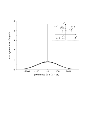
Figure 6: Experimental evidence of the kinetic sampling effect for $m=1$: steady-state preference distribution of the average number of agents holding the identity strategy and its complement, immediately before $t=0$, and $\rho=N=1023$ and averaged over 100000 samples. Inset: The labeling of the time steps in the attractor.

Figure 7: Experimental evidence of the kinetic sampling effect for $m=2$: steady-state preference distribution of the average number of agents holding the XOR strategy $\xi_{a}^{\mu}$ and its complement $\xi_{b}^{\mu}$, immediately before $t=4$, and $\rho=N=511$ and averaged over 50000 samples. Inset: The labeling of the time steps in the attractor.

This effect that favors the cooperation of larger clusters of agents is referred to as the kinetic sampling effect. To describe this effect, we consider the probability of $P_{\rm att}(\Delta{\bf A})$ of step sizes $\Delta{\bf A}$ in the attractor. For convenience, we only consider $\Delta A^{\mu}>0$ for all $\mu$. Assuming that all states of the phase space are equally likely to be accessed by the initial condition, we have

$$P_{\rm att}(\Delta{\bf A})=\sum_{\bf A}P_{\rm att}(\Delta{\bf A},{\bf A}),$$ (35)

where $P_{\rm att}(\Delta{\bf A},{\bf A})$ is the probability of finding the position ${\bf A}$ with displacement $\Delta{\bf A}$ in the attractor. Consider the example of $m=1$, where there is only one step along each axis $A^{\mu}$. The sign reversal condition implies that

$$P_{\rm att}(\Delta{\bf A},{\bf A})=P_{\rm Poi}(\Delta{\bf A})\prod_{\mu}\Theta[-A^{\mu}(A^{\mu}+\Delta A^{\mu})],$$ (36)

where $P_{\rm Poi}(\Delta{\bf A})$ is the Poisson distribution of step sizes, yielding

$$P_{\rm att}(\Delta{\bf A})\propto P_{\rm Poi}(\Delta{\bf A})\prod_{\mu}\Delta A^{\mu}.$$ (37)

We note that the extra factors of $\Delta A^{\mu}$ favor large step sizes. Thus the attractor averages $\langle(\Delta A^{\pm})^{2}\rangle_{\rm att}$, which are required for computing the variance of decisions, are given by

$$\langle(\Delta A^{\pm})^{2}\rangle_{\rm att}=\frac{\langle(\Delta A^{\pm})^{2}\Delta A^{+}\Delta A^{-}\rangle_{\rm Poi}}{\langle\Delta A^{+}\Delta A^{-}\rangle_{\rm Poi}}.$$ (38)

Furthermore, correlation effects come into action when the step sizes become non-self-averaging. There are agents who contribute to both $\Delta A^{+}$ and $\Delta A^{-}$, giving rise to their correlations. Thus, the variance of decisions is higher when correlation effects are considered. In Eq. (14), the strategies of the agents contributing to $\Delta A^{+}$ and $\Delta A^{-}$ satisfy $\xi^{+}_{a}-\xi^{+}_{b}=\pm 2$ and $\xi^{-}_{a}-\xi^{-}_{b}=\mp 2$ respectively. Among the agents contributing to $\Delta A^{+}$, the extra requirement of $\xi^{-}_{a}-\xi^{-}_{b}=\mp 2$ implies that an average of $1/4$ of them also contribute to $\Delta A^{-}$. Hence, the number of agents contributing to both steps is a Poisson variable with mean $\Delta/8$. Similarly, the number of agents exclusive to the individual steps are Poisson variables with means $3\Delta/8$. Algebraically, Eq. (14) can be decomposed as

$$\Delta A^{\pm}=\frac{2}{N}\sum_{a<b}\sum_{r=\pm 1}S_{ab}(-r-\Omega_{a}+\Omega_{b})\delta(\xi_{a}^{\pm}-\xi_{b}^{\pm}+2r)\delta(\xi_{a}^{\mp}-\xi_{b}^{\mp}-2r)$$

$$+\frac{2}{N}\sum_{a<b}\sum_{r=\pm 1}S_{ab}(-r-\Omega_{a}+\Omega_{b})\delta(\xi_{a}^{\pm}-\xi_{b}^{\pm}+2r)[\delta(\xi_{a}^{\mp}-\xi_{b}^{\mp})+\delta(\xi_{a}^{\mp}-\xi_{b}^{\mp}+2r)]\}.$$ (39)

Respectively, the first and terms are equal to $2/N$ times the number of agents, common to both steps $\Delta A^{\pm}$ and exclusive to the individual steps, with means $\Delta/8$ and $3\Delta/8$, as can be verified by a derivation similar to that of Eq. (22) from Eq. (14). Hence the denominator of Eq. (38) is given by

$$\langle\Delta A^{+}\Delta A^{-}\rangle_{\rm Poi}=\frac{4}{N^{2}}\sum_{a_{0},a_{+},a_{-}}\frac{e^{-\frac{\Delta}{8}}}{a_{0}!}\left(\frac{\Delta}{8}\right)^{a_{0}}\frac{e^{-\frac{3\Delta}{8}}}{a_{+}!}\left(\frac{3\Delta}{8}\right)^{a_{+}}\frac{e^{-\frac{3\Delta}{8}}}{a_{-}!}\left(\frac{3\Delta}{8}\right)^{a_{-}}(a_{0}+a_{+})(a_{0}+a_{-}).$$ (40)

Expressing the moments of Poisson variables in terms of their means, we arrive at

$$\langle\Delta A^{+}\Delta A^{-}\rangle_{\rm Poi}=\frac{4}{N^{2}}\left[16\left(\frac{\Delta}{8}\right)^{2}+\frac{\Delta}{8}\right].$$ (41)

Similarly, the numerator of Eq. (38) is given by

$$\langle(\Delta A^{\pm})^{2}\Delta A^{+}\Delta A^{-}\rangle_{\rm Poi}=\frac{16}{N^{4}}\left[256\left(\frac{\Delta}{8}\right)^{4}+240\left(\frac{\Delta}{8}\right)^{3}+40\left(\frac{\Delta}{8}\right)^{2}+\frac{\Delta}{8}\right].$$ (42)

Together we obtain

$$\langle(\Delta A^{\pm})^{2}\rangle_{\rm att}=\frac{2\Delta^{3}+15\Delta^{2}+20\Delta+4}{N^{2}(2\Delta+1)}.$$ (43)

The possible attractor states are given by $A^{\mu}=m_{\mu}/N$ and $m_{\mu}/N-\Delta A^{\mu}$, where $m_{\mu}=1,~{}3,~{}\ldots,~{}N\Delta A^{\mu}-1$. This yields a variance of

$$\frac{\sigma^{2}}{N}=\frac{N}{4}\left\langle\left\{\frac{1}{D}\sum_{\mu=0}^{D-1}\left[\left(\frac{m_{\mu}}{N}\right)^{2}-\Delta A^{\mu}\left(\frac{m_{\mu}}{N}\right)+\frac{1}{2}(\Delta A^{\mu})^{2}\right]-\left[\frac{1}{D}\sum_{\mu=0}^{D-1}\left(\frac{m_{\mu}}{N}-\frac{1}{2}\Delta A^{\mu}\right)\right]^{2}\right\}\right\rangle.$$ (44)

Averaging over the attractor states, we find

$$\frac{\sigma^{2}}{N}=\frac{7\langle(N\Delta A^{+})^{2}\rangle_{\rm att}+7\langle(N\Delta A^{-})^{2}\rangle_{\rm att}-8}{192N},$$ (45)

which gives, on combining with Eq. (43),

$$\frac{\sigma^{2}}{N}=\frac{14\Delta^{3}+105\Delta^{2}+132\Delta+24}{96N(2\Delta+1)}.$$ (46)

When the diversity is low, $\Delta\gg 1$, and Eq. (46) reduces to $\sigma^{2}/N\equiv 7/48\pi\rho$, agreeing with the scaling result of the previous section. When $\rho\sim N$, Eq. (46) has excellent agreement with simulation results, which significantly deviate above the scaling relation, as shown in Fig. 3.

When $\rho\gg N$, Eq. (46) predicts that $\sigma^{2}/N$ should approach $1/4N$. This can be explained as follows. Analysis shows that only those agents holding the identity strategy and its complement can complete both hops along the $A^{\pm}$ axes after they have adjusted their preferences to $\omega+\Omega_{a}-\Omega_{b}=\pm 1$. Since there are fewer and fewer fickle agents in the limit $\rho\gg N$, one would expect that a single agent of this type would dominate the game dynamics, and $\sigma^{2}/N$ would approach $1/4N$.

However, as shown in Fig. 3, the simulation data approaches the limit $0.43/N$ when $\rho\gg N$, significantly higher than $0.25/N$. This discrepancy requires the consideration of the waiting effect, which has been sketched in Wong et al. (2004), and will be explained in details elsewhere.

Next, we turn to the kinetic sampling effects for $m=2$. As shown in Fig. 1(b), the situation is more complicated than that of $m=1$ since there are two steps moving along the direction $A^{1}$ and $A^{2}$. Consider the attractor sequence in Eq. (8). The step $\Delta A(1)$ can initiate from $A^{1}=m_{1}/N$, with $m_{1}=-1,~{}\ldots,~{}-N\Delta A(1)+1$, where for convenience the state labels of the step sizes at time $t$ are implicitly taken to be the historical states $\mu^{*}(t)$. Similarly, the step $\Delta A(5)$ can initiate from $A^{1}=m_{5}/N$, with $m_{5}=1,~{}\ldots,~{}N\Delta A(5)-1$. However, since the two steps are linked by steps along the direction $A^{2}$, their positions are no longer independent. Taking into consideration the many possibilities of their relative displacements make the problem intractable. As shown in Fig. 8, we only consider the most probable case that the two steps are symmetrically positioned, that is, their midpoints have the same $A^{1}$ coordinate. In this case, the possible initial positions of the steps are $A(1)=m_{1}/N$, with $m_{1}=-1,~{}\ldots,~{}-[N\Delta A(1)+N\Delta A(5)]/2+1$, and $A(5)=m_{5}/N$, with $m_{5}=m_{1}+[N\Delta A(1)+N\Delta A(5)]/2$. Thus, the number of possible states along the direction $A^{1}$ is $[N\Delta A(1)+N\Delta A(5)]/4$. Considering the motion in the 4 directions, the total number of possible states is $[N\Delta A(0)/2][(N\Delta A(1)+N\Delta A(5))/4][N\Delta A(2)/2][(N\Delta A(4)+N\Delta A(6))/4]$.

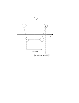
Figure 8: The relative positions of the steps $\Delta A(1)$ and $\Delta A(5)$ for the case $\Delta A(5)>\Delta A(1)$. Here they are shown symmetrically positioned.

Extending the derivation of Eq. (45) to the case of $m=2$, we have

$$\frac{\sigma^{2}}{N}=\frac{N}{256} \Biggl{\{}5\langle\Delta A(0)^{2}\rangle_{\rm att}+5\left\langle\frac{(\Delta A(1)+\Delta A(5))^{2}}{4}\right\rangle_{\rm att}$$ (47)

$$+5\langle\Delta A(2)^{2}\rangle_{\rm att}+5\left\langle\frac{(\Delta A(4)+\Delta A(6))^{2}}{4}\right\rangle_{\rm att}-16\Biggr{\}},$$

where the attractor averages are defined as the Poisson averages weighted by kinetic sampling. For example,

$$\langle\Delta A(0)^{2}\rangle_{\rm att}=\frac{\langle\Delta A(0)[\Delta A(1)+\Delta A(5)]\Delta A(2)[\Delta A(4)+\Delta A(6)]\Delta A(0)^{2}\rangle_{\rm Poi}}{\langle\Delta A(0)[\Delta A(1)+\Delta A(5)]\Delta A(2)[\Delta A(4)+\Delta A(6)]\rangle_{\rm Poi}}.$$ (48)

This requires us to compute Poisson averages such as $\langle\Delta A(t_{1})\cdots\Delta A(t_{k})\rangle_{\rm Poi}$. The following identity for Poisson averages is useful. Consider a universal set of $M$ elements, and the sizes of the sets $B_{1}\cdots B_{k}$ and their intersections are Poisson distributed. Then the expectation of the product $|B_{1}|\cdots|B_{k}|$ is given by

$$\langle|B_{1}|\cdots|B_{k}|\rangle=\prod_{r=1}^{k}\langle|B_{r}|\rangle+\sum_{r<s}\langle|B_{r}\cap B_{s}|\rangle\prod_{u\neq rs}\langle|B_{u}|\rangle+\cdots+\langle|\bigcap_{r=1}^{k}B_{r}|\rangle.$$ (49)

This identity can be proved by writing

$$|B_{1}|\cdots|B_{k}|=\sum_{i_{1}=1}^{M}\cdots\sum_{i_{k}=1}^{M}\Theta(i_{1}\in B_{1})\cdots\Theta(i_{k}\in B_{k})$$ (50)

where $\Theta(i_{r}\in B_{r})$ if $i_{r}\in B_{r}$ and 0 otherwise. In the limit of $M$ approaching infinity, the case that all $i_{r}$ are distinct yields the expectation value in the first term of Eq. (49), the case that $i_{r}=i_{s}$ corresponds to the second term, and the case that all $i_{r}$ are identical corresponds to the last term, and so on.

Therefore, we can write

$$\langle\Delta A(1)\cdots\Delta A(k)\rangle=\left(\frac{2}{N}\right)^{k}\left\{\prod_{r=1}^{k}b_{r}+\sum_{r<s}b_{rs}\prod_{u\neq rs}b_{a}+\cdots+b_{1\cdots+k}\right\}$$ (51)

where $b_{r_{1}\cdots r_{i}}$ is the average number of agents simultaneously contributing to the steps $\Delta A(r_{1})\cdots\Delta A(r_{i})$.

Consider the attractor sequence in Eq. (8). Tracing the time evolution of the cumulative payoffs, the step sizes at $t=2$ and $t=6$, for example, are given by

$$\Delta A(2)=\frac{2}{N}\sum_{a<b}\sum_{r=\pm 1}S_{ab}(-r-\Omega_{a}(2)+\Omega_{b}(2))\delta(\xi_{a}^{3}-\xi_{b}^{3}-2r),$$ (52)

$$\Delta A(6)=\frac{2}{N}\sum_{a<b}\sum_{r^{\prime}=\pm 1}S_{ab}(-r^{\prime}-\Omega_{a}(2)+\Omega_{b}(2)+\xi_{a}^{1}-\xi_{b}^{1}-\xi_{a}^{2}+\xi_{b}^{2}))\delta(\xi_{a}^{2}-\xi_{a}^{2}+2r^{\prime}).$$ (53)

Following the analysis of Eq. (39), we find $b_{2}=b_{6}=\Delta/2$. To find $b_{26}$, we note that the agents shared by the two steps satisfy either $r=r^{\prime}$ and $\xi_{a}^{1}-\xi_{b}^{1}=\xi_{a}^{2}-\xi_{b}^{2}=-2r$, or $r=-r^{\prime}$ and $\xi_{a}^{1}-\xi_{b}^{1}=0$, $\xi_{a}^{2}-\xi_{b}^{2}=2r$. This leads to

$$b_{26}=\sum_{a<b}\sum_{r=\pm 1} \langle S_{ab}(-r-\Omega_{a}(2)+\Omega_{b}(2))\rangle\delta(\xi_{a}^{3}-\xi_{b}^{3}-2r)$$ (54)

$$\times\{\delta(\xi_{a}^{1}-\xi_{b}^{1}+2r)\delta(\xi_{a}^{2}-\xi_{b}^{2}+2r)+\delta(\xi_{a}^{1}-\xi_{b}^{1})\delta(\xi_{a}^{2}-\xi_{b}^{2}-2r)\}.$$

The two terms in this expression consist of the contributions to $\Delta A(2)$, with the extra restrictions of $\xi_{a}^{1}-\xi_{b}^{1}=\xi_{a}^{2}-\xi_{b}^{2}=-2r$, or $\xi_{a}^{1}-\xi_{b}^{1}=0$ and $\xi_{a}^{2}-\xi_{b}^{2}=2r$ respectively. Since $\xi_{a}^{\mu}-\xi_{b}^{\mu}=\pm 2r$ and 0 with probabilities $1/4$ and $1/2$ respectively, we get $b_{26}=3\Delta/32$. Other parameters are listed in Table 4. This enables us to find

$$\langle\Delta A(0)[\Delta A(1)+\Delta A(5)][\Delta A(4)+\Delta A(6)]\Delta A(2)\rangle_{\rm Poi}$$ (55)

$$= \frac{1}{8N^{4}}\left(32\Delta^{4}+84\Delta^{3}+\frac{169}{4}\Delta^{2}+2\Delta\right).$$

Other expressions appearing in Eq. (47) can be found similarly. The final result is

$$\frac{\sigma^{2}}{N}=\frac{160\Delta^{5}+1680\Delta^{4}+4772\Delta^{3}+\frac{272061}{64}\Delta^{2}+\frac{7583}{8}\Delta+17}{64N(32\Delta^{3}+84\Delta^{2}+\frac{169}{4}\Delta+2)}.$$ (56)

Since the attractor sequence in Eq. (9) yields the same result, Eq. (56) is the sample average of the variance. When the diversity is low, $\Delta\gg 1$, and Eq. (56) reduces to $\sigma^{2}/N=5/32\pi\rho$, agreeing with the scaling result of the previous section. When $\rho\sim N$, Eq. (56) shows that the introduction of kinetic sampling significantly improves the theoretical agreement with simulation results, as shown in Fig. 4. When $\rho\gg N$, Eq. (56) implies that $\sigma^{2}/N$ approaches $17/128N$. This result is not valid since it is below the lowest possible result of $1/4N$ when each step is excuted by the strategy switching of only one agent. The discrepency can be traced to the approximation that the average number of states along the direction $A^{1}$ is $[N\Delta A(1)+N\Delta(5)]/2$, which is not precise for small steps. For example, it can take half integer values. We will not pursue this issue further since, in any case, waiting effects have to be taken into account in analysing the case $\rho\gg N$.

$\Delta/2$	$b_{0},b_{1},b_{2},b_{4},b_{5},b_{6}$
$\Delta/4$	$b_{15},b_{46}$
$\Delta/8$	$b_{01},b_{06},b_{12},b_{14},b_{16},b_{24},b_{45},b_{56}$
$3\Delta/32$	$b_{02},b_{04},b_{05},b_{25},b_{26}$
$\Delta/16$	$b_{015},b_{046},b_{125},b_{246}$
$\Delta/32$	$b_{012},b_{014},b_{016},b_{056},b_{124},b_{126},b_{245}$
$3\Delta/128$	$b_{024},b_{026}$
$\Delta/64$	$b_{025}$
$\Delta/128$	$b_{0124},b_{0126}$
$\Delta/64$	$b_{0125},b_{0246}$

Table 4: Values of $b_{t_{1}\cdots t_{r}}$ for the attractor sequence in Eq. (8). The steps at $t=3$ and $t=4$ are identical, so are the steps at $t=6$ and $t=7$. Other unlisted parameters are zero.

In summary, we have explained the reduction of variance by the reduction of the fraction of fickle agents when diversity increases. The theoretical analysis from Sections III to V spans the 3 regimes of small $R$, $\rho^{-1}$ scaling, and kinetic sampling, yielding excellent argreement with simulations over 7 decades.

It is natural to consider whether the results presented here can be generalized to the case of the exogenous MG, in which the information $\mu(t)$ was randomly and independently drawn at each time step $t$ from a distribution $\rho^{\mu}=1/D$ Challet et al. (2000). This is different from the present endogenous version of the MG, in which the information is determined by the sequence of the winning bits in the game history. The similarities and differences between the behavior of those two versions have been a topic of interest in the literature Cavagna (1999); Johnson et al. (1999b); Challet et al. (2000); Zheng and Wang ; Lee (2001); Metzler (2002); web . Here we compare their behavior in games of small $m$ using the phase space we introduced.

In the scaling regime, the picture that the states of the game are hopping between hypercubes in the phase space remains valid, as shown in Fig. 9 for $m=1$. At the steady state, the attractor consists of hoppings along all edges of a hypercube, in contrast to the endogenous case, in which only a fraction of hypercube vertices belong to the attractor. The behavior in the scaling regime depends on the scaling of the step sizes with diversity, rather than the actual sequence of the steps. Consequently, the behavior is the same as the endogenous game. In the kinetic sampling regime, the physical picture that larger steps are more likely to be trapped remains valid, and the behavior remains qualitatively similar to the endogenous case.

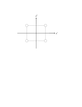
Figure 9: An attractor of the exogenous Minority Game for $m=1$.

VI The Fraction of Fickle Agents

This physical picture of the diversity effects is further illustrated by considering the fraction $f_{\rm fi}$ of fickle agents when the game has reached the steady state. They hold strategy pairs whose preferences are distributed near zero, and change sign during the attractor dynamics. As confirmed in Figs. 10 and 11, three regimes of behavior exist.

Figure 10: The dependence of the fraction of fickle agents on the randomness $R$ at $m=1$ and $s=2$. Notations are the same as those of Fig. 3.

Figure 11: The dependence of the fraction of fickle agents on the randomness $R$ at $m=2$ and $s=2$. Notations are the same as those of Fig. 3.

In the multinomial regime, we can make use of the explicit knowledge about the attractor sequence and the evolution of the payoffs in the attractor dynamics. Consider the example of $m=1$. We count the type of fickle agents labeled by the strategy pairs $a<b$ and bias $\omega$ for all $t$, with preferences

$$\omega+\Omega_{a}(t)-\Omega_{b}(t)=\pm 1~{}~{}~{}~{}{\rm and}~{}~{}~{}~{}\xi_{a}^{\mu}-\xi_{b}^{\mu}=\mp 2{\rm sgn}A^{\mu}(t),$$ (57)

where $\mu=\mu^{*}(t)$. Equivalently, we have

$$\omega=-\Omega_{a}(t)+\Omega_{b}(t)-\frac{1}{2}(2\sigma(t)-1)(\xi_{a}^{\mu^{*}(t)}-\xi_{b}^{\mu^{*}(t)}),$$ (58)

where $\Omega_{a}(t)$ is updated by

$$\Omega_{a}(t+1)=\Omega_{a}(t)+\xi_{a}^{\mu^{*}(t)}[2\sigma(t)-1].$$ (59)

This enables us to count the types directly from the knowledge of the attractor sequences, such as Eqs. (7) and (8), without having to know the step sizes. Results for $m=1$ and $m=2$ are listed in Tables 5 and 6 respectively. Note that the values in the tables depend on the convention of ordering the strategies $a<b$, and here the convention of Eq. (2) is adopted. Other conventions may classify the types with bias $\omega$ as $-\omega$, or vice versa. Since the average number of fickle agents of each type is given by Eq. (3), $f_{\rm fi}$ can then be obtained by summing up the contribution from each type.

$\omega$	(a)	(b)	(c)	(d)	Total
$-3$	1	0	0	0	1
$-1$	5	4	0	3	12
1	1	3	6	3	13
3	0	0	1	1	2
Total	7	7	7	7

Table 5: The number of types of fickle agents for the attractors (a)-(d) in Fig. 5.

Consider the example of $m=1$. Table 5 shows that there are 7 types of fickle agents for each attractor shown in Fig. 5. Averaging over initial states, we find that an average of $25/4$ types consist of agents with biases $\omega=\pm 1$, and an average of $3/4$ types with $\omega=\pm 3$, this result being independent of the ordering of $a<b$. Since the average number of agents holding strategy pair $a<b$ is $N/8$, we have

$$f_{\rm fi}=\frac{25}{32}\binom{R}{\frac{R-1}{2}}\frac{1}{2^{R}}+\frac{3}{32}\binom{R}{\frac{R-3}{2}}\frac{1}{2^{R}}.$$ (60)

For $m=2$, the number of types of fickle agents for the 16 attractors in Table 3 are listed in Table 6. There are 194 types of fickle agents for each attractor. The fraction of fickle agents is given by

$$f_{\rm fi}=\frac{1121}{1024}\binom{R}{\frac{R-1}{2}}\frac{1}{2^{R}}+\frac{373}{1024}\binom{R}{\frac{R-3}{2}}\frac{1}{2^{R}}+\frac{55}{1024}\binom{R}{\frac{R-5}{2}}\frac{1}{2^{R}}+\frac{3}{1024}\binom{R}{\frac{R-7}{2}}\frac{1}{2^{R}}.$$ (61)

In the scaling regime $\rho\sim 1$, we consider the limit of $R\sim N$ in Eq. (60), and obtain for $m=1$,

$$f_{\rm fi}=\frac{7}{8}\sqrt{\frac{2}{\pi R}}.$$ (62)

Similarly, from Eq. (61), we have for $m=2$,

$$f_{\rm fi}=\frac{97}{64}\sqrt{\frac{2}{\pi R}}.$$ (63)

Attractor	1	2	3	4	5	6	7	8	9	10	11	12	13	14	15	16	Total
$\omega=-7$	0	0	0	0	0	0	0	0	0	0	0	0	0	0	0	1	1
$\omega=-5$	0	0	0	0	0	2	0	3	0	1	1	4	0	6	4	9	30
$\omega=-3$	0	3	5	10	8	16	16	23	7	20	22	28	24	33	33	38	286
$\omega=-1$	19	42	42	54	52	59	69	66	76	73	76	75	91	84	94	85	1057
$\omega=1$	120	87	92	71	93	70	66	59	90	72	72	60	75	55	54	49	1185
$\omega=3$	48	50	44	46	37	37	36	33	21	25	20	24	4	15	9	11	460
$\omega=5$	7	11	10	12	4	9	7	9	0	3	3	3	0	1	0	1	80
$\omega=7$	0	1	1	1	0	1	0	1	0	0	0	0	0	0	0	0	5
Total	194	194	194	194	194	194	194	194	194	194	194	194	194	194	194	194

Table 6: The number of types of fickle agents for the 16 attractors in Table 3 at $m=2$.

In the kinetic sampling regime, the fraction of fickle agents for $m=1$ is obtained by replacing $(\Delta A^{\pm})^{2}$ in the numerator of Eq. (38) by $(a_{0}+a_{+}+a_{-})/N$, following the notation used in Eq. (40). The result is

$$f_{\rm fi}=\frac{14\Delta^{2}+39\Delta+8}{8N(2\Delta+1)}.$$ (64)

In the limit of low diversity, $\Delta\gg 1$ and Eq. (64) reduces to Eq. (62). In the limit of high diversity, $\Delta\ll 1$ and $f_{\rm fi}$ approaches $1/N$, implying that a single agent would dominate the game dynamics. However, since waiting effects are neglected, this result is considerably lower than the simulation results.

For $m=2$, the fraction of fickle agents is given by the size of the union set of fickle agents at all steps,

$$f_{\rm fi}=\frac{1}{N}\left\langle\sum_{r}b_{r}-\sum_{r<s}b_{rs}+\sum_{r<s<u}b_{rsu}\cdots\right\rangle_{\rm att}$$ (65)

where

$$\langle b_{r_{1}\cdots r_{i}}\rangle_{\rm att}=\frac{\langle\Delta A(0)[\Delta A(1)+\Delta A(5)]\Delta A(2)[\Delta A(4)+\Delta A(6)]b_{r_{1}\cdots r_{i}}\rangle_{\rm Poi}}{\langle\Delta A(0)[\Delta A(1)+\Delta A(5)]\Delta A(2)[\Delta A(4)+\Delta A(6)]\rangle_{\rm Poi}}.$$ (66)

The result is

$$f_{\rm fi}=\frac{1552\Delta^{4}+8170\Delta^{3}+\frac{80905}{8}\Delta^{2}+2801\Delta+64}{32N(32\Delta^{3}+84\Delta^{2}+\frac{169}{4}\Delta+2)}.$$ (67)

In the limit of low diversity, $\Delta\gg 1$ and Eq. (67) reduces to Eq. (63). In the limit of high diversity, $f_{\rm fi}$ approaches $1/N$. However, by tracing the types of fickle agents switching strategies at each time step, one cannot find any single type of agents who can contribute to the dynamics of all steps. In fact, the minimum number of agents that can complement each other to complete the dynamics is 2. For example, one agent can complete the steps at $t=0$, 1, 2, 3, 4, while the other one can complete the steps $t=5$, 6, 7. Hence the asymptotic limit of $f_{\rm fi}=1/N$ is not valid. The source of the discrepancy is the same as that for the invalid result of the asymptotic variance of decisions explained in the previous section.

As shown in Figs. 10 and 11, the theoretical predictions are confirmed by simulations, except in the regime of extremely high diversity, where waiting effects have to be taken into account Wong et al. (2004).

VII Convergence Time

Many properties of the system dependent on the transient dynamics also depend on its diversity. For example, since diversity reduces the fraction of agents switching strategies at each time step, it also slows down the convergence to the steady state. Hence the convergence time increases with diversity.

We consider the example of $m=1$. The dynamics of the game proceeds in the direction which reduces the variance Challet et al. (2000). In the multinomial regime, the initial position of $A^{\mu}$ in the phase space lies in the attractor. Convergence to the steady state is almost instant. Starting from the initial state 0, the convergence time is 2, 0, 0, 1 in the 4 respective quadrants of the phase space in Fig. 1. For the initial state 1, the game has the same set of convergence times, except that the order described is permuted. Hence, the convergence time is 2, 1 and 0 with probabilities $1/4$, $1/4$ and $1/2$ respectively, yielding the average convergence time of $3/4$.

In the scaling regime, it is convenient to make use of the rectilinear nature of the motion in the phase space. We divide the phase space into hypercubes with dimensions $\sqrt{2/\pi R}$. Starting from the initial state 0, the convergence paths are shown in Fig. 12. The convergence time $\tau$ of an initial state from inside a hypercube is the number of steps it hops between the hypercubes on its way to the attractor, as shown in Fig. 13.

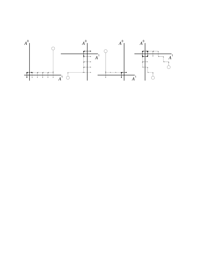
Figure 12: The convergence paths starting from the initial state 0 in the 4 quadrants of the phase space for $m=1$.

Figure 13: The dependence of the convergence time on the initial position in the phase space for $m=1$, starting from the initial state 0. The dimensions of the hypercubes are $\sqrt{2/\pi R}$. Inset: The 3 regimes of convergence time in the continuum limit.

In general, the convergence time is given by the following cases: (a) $3x+y+2$ for $x\geq 0$ and $y\geq-x-1$, where $x=\left\lfloor\sqrt{\frac{\pi R}{2}}A^{1}(0)\right\rfloor$ and $y=\left\lfloor\sqrt{\frac{\pi R}{2}}A^{0}(0)\right\rfloor$; (b) $-x-3y-4$ for $y\leq-2$ and $y\leq-x-2$; (c) $-x+y-1$ for $x\leq-2$ and $y\geq-1$; (d) $y$ for $x=-1$ and $y\geq 0$; (e) 0 for $x=y=-1$.

The average convergence time is then obtained by averging over the Gaussian distribution of the initial $A^{\mu}(0)$ with mean 0 and variance $1/N$. When $\rho$ is small, the initial positions are mainly distributed around the origin, reducing the convergence time to that of the multinomial regime. When $\rho$ is large, the initial positions are broadly distributed among many hypercubes in the phase space, and one can take a continuum approximation as shown in the inset of Fig. 13. Thus, the average convergence time is given by

$$\tau= \sqrt{\frac{\pi R}{2N}}\Biggl{\{}\int_{0}^{\infty}Dx\int_{-x}^{\infty}Dy(3x+y)+\int_{-\infty}^{0}Dy\int_{-\infty}^{-y}Dx(-x-3y)$$ (68)

$$+\int_{-\infty}^{0}Dx\int_{0}^{\infty}Dy(-x+y)\Biggr{\}},$$

where $Dx\equiv dx~{}e^{-\frac{x^{2}}{2}}/\sqrt{2\pi}$ is the Gaussian measure. The result is

$$\tau=(2+\sqrt{2})\sqrt{\rho}.$$ (69)

As shown in Fig. 14, there is an excellent agreement between theory and simulations.

The $\rho^{1/2}$ dependence of the convergence time can be interpreted as follows. In the scaling regime, since the step size in the phase space scales as $1/\sqrt{R}$ and the initial position of $A^{\mu}$ has components scaling as $1/\sqrt{N}$, the convergence time should scale as $(1/\sqrt{N})/(1/\sqrt{R})\sim\rho^{1/2}$. This scaling relation remains valid in the kinetic sampling regime where $\rho\sim N$, since kinetic sampling only affects the description of the attractor, rather than the transient behavior.

VIII Wealth Spread

Another system property dependent on the transient is the distribution of wealth or resources, especially those among the frozen agents (that is, agents who do not switch their strategies at the steady state). Since the system dynamics reaches a periodic attractor, they have constant average wealth at the steady state. Hence any spread in their wealth distribution is a consequence of the transient dynamics.

To simiplify the analysis, we only consider the agents who hold identical strategy pairs. Since they never switch strategies, and both outputs 1 and 0 have equal occurence at the attractor, their wealth averaged over a period becomes a constant, and their wealth is equal to the cumulative payoff of the identical strategies they hold.

In the multinomial regime, the wealth of agents holding identical strategies $a$ is given by Eq. (16), where $k_{\mu}(t)$ are listed in Table 1. For $m=1$, the periodic average $\langle\Omega_{a}\rangle_{t}$ of the cumulative payoffs of strategies and their variances $\langle\langle\Omega_{a}\rangle_{t}^{2}\rangle_{a}$ are listed in Table 7. Thus, the wealth spread $W$ is the variance $\langle\langle\Omega_{a}\rangle_{t}^{2}\rangle_{a}$ of $\langle\Omega_{a}\rangle_{t}$, averaged over the four strategies and the four attractors, and is equal to $5/8$.

	$\xi_{a}^{1}$	$\xi_{a}^{0}$	(a)	(b)	(c)	(d)
$\langle\Omega_{0}\rangle_{t}$	-1	-1	1	0	-1	0
$\langle\Omega_{1}\rangle_{t}$	1	-1	-$\frac{1}{2}$	$\frac{1}{2}$	-$\frac{1}{2}$	-$\frac{3}{2}$
$\langle\Omega_{2}\rangle_{t}$	-1	1	$\frac{1}{2}$	-$\frac{1}{2}$	$\frac{1}{2}$	$\frac{3}{2}$
$\langle\Omega_{3}\rangle_{t}$	1	1	-1	0	1	0
$\langle\langle\Omega_{a}\rangle^{2}_{t}\rangle_{a}$			$\frac{5}{8}$	$\frac{1}{8}$	$\frac{5}{8}$	$\frac{9}{8}$

Table 7: The variance $\langle\langle\Omega\rangle_{t}^{2}\rangle_{a}$ of the periodic average of wealth of the 4 strategies, for the 4 attractors of $m=1$.

In the scaling regime, the initial position may be located away from the origin of the phase space. Using the hypercube picture of the transient motion, we can work out the cumulative payoffs of the strategies by considering their changes when their initial position shift to successive neighboring hypercubes. The distribution of wealth variance is shown in Fig. 15. In general, if $x=\left\lfloor\sqrt{\frac{\pi R}{2}}A^{1}(0)\right\rfloor$ and $y=\left\lfloor\sqrt{\frac{\pi R}{2}}A^{0}(0)\right\rfloor$, then the average wealth of the 4 strategies in Table 7 are $x+y+1$, $-x+y-1/2$, $x-y+1/2$ and $-x-y-1$ respectively. This leads to a wealth spread of $x^{2}+y^{2}+3x/2+y/2+5/8$.

The value of $W$ is then obtained by averaging the wealth spread over the Gaussian distribution of the initial positions in the phase space, each component $A^{\mu}(0)$ with mean 0 and variance $1/N$. When $\rho$ is small, the initial positions are mainly distributed around the origin, reducing the wealth spread $W$ to the value at the multinomial regime. When $\rho$ is large, the initial positions are broadly distributed among many hypercubes in the phase space. Applying the continuum approximation,

$$W=\frac{\pi R}{2N}\int Dx\int Dy(x^{2}+y^{2})=\pi\rho.$$ (70)

The same scaling relation applies to the kinetic sampling regime. As shown in Fig. 16, agreement between theory and simulations is excellent. Note that the behavior closely resembles that of the convergence time in Fig. 14, showing that it is a transient behavior.

Figure 14: The dependence of the average convergence time on the diversity at $m=1$.

Figure 15: The dependence of the variance of wealth among the agents holding identical strategies on the initial position in the phase space for $m=1$. The dimensions of the hypercubes are $\sqrt{2/\pi R}$.

Figure 16: The dependence of the variance of wealth on the diversity among the agents holding identical strategies for $m=1$.

IX Discussions

We have studied the effects of diversity in the initial preference of strategies on a game with adaptive agents competing selfishly for finite resources. Introducing diversity is both useful in modeling agent behavior in economic markets, and as a means to improve distributed control. We find that it leads to the emergence of a high system efficiency. We have made use of the small memory sizes $m$ to visualize the motion in the phase space. Scaling of step sizes accounts for the dependence of the efficiency on the diversity in the scaling regime ($\rho\sim 1$), while kinetic sampling effects have to be considered at higher diversity, yielding theoretical predictions with excellent agreement with simulations up to $\rho\sim N$. However, when diversity increases further, waiting effects have to be considered Wong et al. (2004) and will be discussed in details elsewhere. The variance of decisions decreases with diversity, showing that the maladaptive behavior is reduced. On the other hand, the convergence time and the wealth spread increases with diversity.

While the present results apply mostly to the cases of small $m$, qualitative predictions can be made about higher values of $m$. An extension of Eq. (23) shows that when $\alpha$ increases, the step size becomes smaller and smaller in the asymptotic limit. There is a critical slow down since the convergence time diverges at $\alpha_{c}=\pi^{-1}=0.3183$ Wong et al. (2004). When $\alpha$ exceeds $\alpha_{c}$, the step size vanishes before the system reaches the attractor near the origin, so that the state of the system is trapped at locations with at least some components being nonzero. The interpretation is that when $\alpha$ is large, the distribution of strategies become so sparse that motions in the phase space cannot be achieved by the switching of strategies. This agrees with the picture of a phase transition from the symmetric to asymmetric phase when $\alpha$ increases Challet and Marsili (1999). It is interesting to note that the value of $\alpha_{c}$ is close to the value of 0.3374 obtained by the continuum approximation Challet et al. (2000); Sherrington et al. (2002b) or batch update Coolen et al. (2001) using linear payoff functions.

Another extension to general $m$ applies to the symmetric phase of the exogenous game. In this case the attractor can be approximated by a hyperpolygon enclosing the origin of the phase space. Using a generating function approach, we have computed the variance of decisions, taking into account the scaling of step sizes and kinetic sampling; the analysis will be presented elsewhere. The results agree qualitatively with simulations of both the exogenous and endogenous games, except for values of $\alpha$ close to $\alpha_{c}$. In fact, when $\alpha$ increases, there is an increasing fraction of samples in which the attractors are more complex than hyperpolygons. For example, in the endogenous case, there is an increasing fraction of attractors whose periods are no longer $2D$ Caridi and Ceva (2003). Instead, their periods become multiples of the fundamental period $2D$. It is remarkable that the population variance is not seriously affected by the structural change of the attractor, probably because the dynamical description of such long-period attractors have strong overlaps with those of several distinct attractors of period $2D$.

Besides step payoffs, the case of linear payoffs is equally interesting. In fact, the latter case has also been considered recently, and the variance of decisions is also found to decrease with diversity Ting . There are significant differences between the two cases, though, indicating that agents striving to maximize different payoffs cause the system to self-organize in different fashions. The details will be explained elsewhere.

From the viewpoint of game theory, it is natural to consider whether the introduction of diversity assists the game to reach a Nash equilibrium, in contrast to the case of the homogeneous initial condition where maladaptation is prevalent. It has been verified that Nash equilibria consist of pure strategies Challet et al. (2000). Hence all frozen agents have no incentives to switch their strategies. In fact, since the dynamics in the attractor is periodic for small $m$, with states $\pm 1$ appearing once each in response to each historical string, the payoffs of all strategies become zero when averaged over a period. Thus, the Nash equilibrium is approached in the sense that the fraction of fickle agents decreases with increasing diversity. In the limit of $\rho\gg N$, it is probable that only one fickle agent switches strategy at each step in the attractor, as predicted by Eq. (64) for the case $m=1$. In this case, agents who switch their decisions cannot increase their payoffs, since on switching, the minority ones would become losers, and the majority ones would change the minority side to majority and lose. (Though the fickle agents are not playing pure strategies, this argument implies that their payoffs are the same as if they are doing so.) Then a Nash equilibrium is reached exactly. However, as mentioned previously, waiting effects become important in the extremely diverse limit, and there are cases that more than one fickle agent contribute to a single step in the attractor dynamics, and Nash equilibrium cannot be reached.

The combination of scaling and kinetic sampling in accounting for the steady state properties of the system illustrates the importance of dynamical considerations in describing the system behavior, at least for small values of $m$. We anticipate that these dynamical effects will play a crucial role in explaining the system behavior in the entire symmetric phase, since when $\alpha$ increases, the state motion in a high dimensional phase space can easily shift the tail of the cumulative payoff distributions to the verge of strategy switching, leading to the sparseness condition where kinetic sampling effects are relevant. Due to their generic nature inherent in multi-agent systems with dynamical attractors formed by the collective actions of many adaptive agents, we expect that these effects are relevant to minority games with different payoff functions and updating rules, as well as other multi-agent systems with adaptive agents competing for limited resources.

The sensitivity of the steady state to the initial conditions has implications to adaptation and learning in games. First, when the MG is used as a model of financial markets, it shows that the maladaptive behavior is, to a large extent, an artifact of the homogeneous initial condition. In practice, when agents enter the market with diverse views on the values of the strategies, the corresponding initial condition should be randomized, and the market efficiency is better than previously believed. Second, when the MG is used as a model of distributed load balancing, the present study illustrates the importance to adopt diverse initial conditions in order to attain the optimal system efficiency. The effect is reminiscent of the dynamics of learning in neural networks, in which case an excessive learning rate might hinder the convergence to optimum Hertz et al. (1981).