Electronic self-energy and triplet pairing fluctuations in the vicinity of a ferromagnetic instability in 2D systems: the quasistatic approach

Abstract

The self-energy, spectral functions and susceptibilities of 2D systems with strong ferromagnetic fluctuations are considered within the quasistatic approach. The self-energy at low temperatures $T$ has a non-Fermi liquid form in the energy window $|\omega|\lesssim\Delta_{0}$ near the Fermi level, where $\Delta_{0}$ is the ground-state spin splitting for magnetically ordered ground state, and $\Delta_{0}\propto T^{1/2}\ln^{1/2}(v_{F}/T)$ in the quantum critical regime ($v_{F}$ is the Fermi velocity). Spectral functions have a two-peak structure at finite $T$ above the magnetically ordered ground state, which implies quasi-splitting of the Fermi surface in the paramagnetic phase in the presence of strong ferromagnetic fluctuations. The triplet pairing amplitude in the quasistatic approximation increases with increasing correlation length; at low temperatures $T\ll\Delta_{0}$ the vertex corrections become important and the Eliashberg approach is not justified. The results for the spectral properties and susceptibilities in the quantum critical regime near charge- (spin-) instabilities with large enough correlation length $\xi\gg(T/v_{F})^{-1/3}$ are obtained.

I Introduction

Anomalous non-Fermi-liquid behavior of correlated low-dimensional electron systems has attracted much attention during the last decade. This behavior is usually connected with the violation of the quasiparticle (qp) concept in some energy window around the Fermi level. A prominent example is the pseudogap phenomenon observed in underdoped high-T_c compounds [1]. While antiferromagnetic (AFM) fluctuations may be responsible for non-Fermi-liquid behavior and superconducting pairing in cuprates, there is number of systems where ferromagnetic (FM) fluctuations may play an important role. In particular, FM fluctuations may be important in some triplet superconductors, such as UGe${}_{2},$ ZrZn₂ and Sr₂RuO₄. These systems motivate studies of electronic properties in the vicinity of a FM instability and their influence on the triplet superconductivity.

Although many results exist for the electronic properties in the vicinity of an AFM state [2, 3, 4, 5, 6, 7, 8], much less is known about the evolution of quasiparticle properties near the FM instability. An $\varepsilon^{2/3}$ energy dependence of the self-energy at the quantum critical point (QCP) can be derived from calculations in the context of gauge field theories [9], the phase separation problem [10], and the Pomeranchuk instability [11], which are expected to have the same structure of self-energy corrections as a FM instability. The breakdown of the qp concept at the QCP is even more apparent at finite temperatures. It was demonstrated for fermions interacting with a gauge field that the imaginary part of the self-energy in a non-self-consistent calculation diverges at the Fermi level at $T>0$ as a consequence of the divergence of the gauge field propagator at zero momentum and frequency [9]. Similar behavior induced by the divergence of the static uniform spin susceptibility $\chi({\bf 0},0)$ can be expected for the zero-momentum particle-hole instabilities of fermion systems with short-range interactions. This behavior can be especially pronounced in the renormalized classical (RC) regime [12], where the correlation length $\xi$ is exponentially large.

The self-energy and the spectral functions in the RC regime in the vicinity of a FM instability were previously studied within the two-particle self-consistent (TPSC) approximation [13, 14], one-loop functional renormalization group (fRG), and Ward-identity approaches [14]. It was argued, that spectral functions have two-peak structure analogously to the vicinity of an AFM instability[6]. Contrary to the situation in the vicinity of an AFM instability, however, the abovementioned two-peak structure of the spectral functions does not imply strong suppression of the density of states at the Fermi level, but leads to the quasi-splitting of the Fermi surface at low $T$ already in the paramagnetic phase [14]. While the treatment based on the TPSC and one-loop fRG approaches does not account for the feedback of the self-energy effects, the analysis of the self-energy and vertex corrections using Ward identities has shown [14] that these two types of effects almost cancel each other, and therefore resulting spectral functions closely resemble their form in non-self-consistent approaches.

These anomalous spectral properties may have a profound effect on the triplet superconductivity. One can expect that due to strong FM fluctuations in the RC regime the triplet pairing will be mostly enhanced at the new preformed Fermi surfaces. Anomalous spectral properties may have important influence also in quantum-critical (QC) regime [12], where the quasi-splitting of the FS is absent. Previous investigations of this regime [15, 16, 17] neglected vertex corrections, which may be important for large enough correlation length.

To consider anomalies of electronic properties and their impact on the triplet superconductivity, one needs a tool which is able to consider self-energy and vertex corrections on the same foot. The abovementioned self-consistent treatment of self-energy and vertex corrections near a FM instability was performed only to first order in $1/M$, $M$ being the number of spin components ($M=3$ for the Hubbard model). It appears important to investigate spectral properties in the vicinity of FM instability beyond the leading order in $1/M$ to verify whether the near-cancellation of the self-energy and vertex corrections persists also in higher orders of the $1/M$ expansion and to investigate the effect of the anomalous properties on the triplet superconductivity.

Due to an almost static character of spin fluctuations at large correlation length, a useful nonperturbative tool for calculation of the spectral properties and susceptibilities in this case is the quasistatic approach. This approach was originally proposed for the summation of diagrammatic series for the self-energy of one-dimensional (1D) systems in the vicinity of the charge-density wave instability [18] and further developed for 2D systems in the vicinity of an AFM instability [3, 19]. The quasistatic approach allows to sum up the most important series of static contributions to the self-energy and interaction vertices. This approach becomes exact in the limit $\xi\rightarrow\infty,\$and can be applied to study spectral properties in the RC and QC regime, provided that the correlation length is sufficiently large, $(\xi/a)^{-1}\ll(T/v_{F})^{1/3},$ where $v_{F}$ is the Fermi velocity, $a$ is the lattice constant (the latter criterion follows from the comparison of static contributions to the scattering rate $\sim T\xi/a$ with the dynamic contributions proportional to $v_{F}(T/v_{F})^{2/3},$ cf. Ref. [14]). Although the quasistatic approach was applied previously to systems in the vicinity of a FM instability [20], only the form of spectral functions was analyzed, the self-energy, magnetic and triplet pairing susceptibilities being not investigated.

In the present paper we apply the quasistatic approach to 2D systems with nonsingular density of states, which are on the verge of a ferromagnetic instability, to study spectral properties and the possibility of triplet pairing in these systems. In Sect. II we concentrate on the analytical results for spectral properties and susceptibilities for linear electronic dispersion at $\xi\rightarrow\infty$ and compare these results with the results at finite correlation length. In Sect. III we consider the two-particle properties: magnetic susceptibility and the susceptibility with respect to triplet pairing. In Sect. IV we discuss the application of the results to the quantum-critical regime. Finally, in Sect. V we summarize main results of the paper.

II Spectral properties in the vicinity of ferromagnetic instability

We consider a spin-fermion model [2, 3]

$$Z[\eta] = \int D[c,c^{\dagger}]D[{\bf S}]\exp(-{\cal S}[c,{\bf S},\eta])$$ (1)

$${\cal S}[c,{\bf S},\eta] = \sum_{k}\left[c_{k\sigma}^{\dagger}(i\omega_{n}-\varepsilon_{{\bf k}})c_{k\sigma}-(c_{k\sigma}^{\dagger}\eta_{k\sigma}+\eta_{k\sigma}^{\dagger}c_{k\sigma})\right]$$ (4)

$$\ +T^{-1}\sum_{q}(\chi_{q}^{-1}+U^{2}\Pi_{q})({\bf S}_{q}{\bf S}_{-q})$$

$$\ +UT^{-1}\sum_{kk^{\prime}}{\bf S}_{k-k^{\prime}}\sigma_{\sigma\sigma^{\prime}}c_{k\sigma}^{\dagger}c_{k^{\prime}\sigma^{\prime}}$$

where $q=({\bf q},i\omega_{n})$ and similar for $k,$ $\omega_{n}=(2n+1)\pi T$ are fermionic Matsubara frequencies, $\varepsilon_{{\bf k}}$ is the electronic dispersion, $\sigma_{\sigma\sigma^{\prime}}$ are Pauli matrices, $\chi_{q}=\Pi_{q}/(1-U\Pi_{q})$ is the dynamical spin susceptibility,

$$\Pi_{{\bf q},i\omega_{n}}=\sum_{{\bf k}}\frac{f(\varepsilon_{{\bf k}+{\bf q}})-f(\varepsilon_{{\bf k}})}{i\omega_{n}-\varepsilon_{{\bf k}+{\bf q}}+\varepsilon_{{\bf k}}}$$ (5)

is the bare polarization operator, $f(\varepsilon)$ is the Fermi distribution function, $U$ is the strength of the interaction of electrons with the collective magnetic excitations, the lattice constant $a=1$. Although this model was originally proposed as phenomenological model for systems with strong AFM fluctuations, it can be applied for systems with strong FM fluctuations as well. Generally speaking, the interaction $U$ differs from the bare on-site Coulomb repulsion because of contributions of the channels of electron-electron scattering different from particle-hole one, therefore $U$ should be considered as an effective interaction. The counterterm proportional to $U^{2}\Pi_{q}$ keeps the renormalized spin-spin propagator equal to $\chi_{q}$ (see below). The rigorous derivation of the model (4) from the microscopic Hubbard model will be considered elsewhere [22].

Integrating out fermions from (4), we obtain

$$Z[\eta] = \int D[{\bf S}]\exp(-{\cal S}_{eff}[{\bf S},\eta])$$ (6)

$${\cal S}_{eff}[{\bf S},\eta] = T^{-1}\sum_{q}\chi_{q}^{-1}{\bf S}_{q}{\bf S}_{-q}-\ln\det[-G_{kk^{\prime}}^{-1}({\bf S})]$$ (8)

$$+U^{2}T^{-1}\sum_{q}\Pi_{q}{\bf S}_{q}{\bf S}_{-q}+\sum_{kk^{\prime}}\eta_{k}^{\dagger}G_{kk^{\prime}}^{-1}({\bf S})\eta_{k^{\prime}}$$

where

$$G_{kk^{\prime}}^{-1}({\bf S})=(i\omega_{n}-\varepsilon_{{\bf k}})\delta_{\sigma\sigma^{\prime}}\delta_{kk^{\prime}}+U{\bf S}_{k-k^{\prime}}\sigma_{\sigma\sigma^{\prime}}$$ (9)

In the following we expand $\ln\det(-G^{-1})$ in Eq. (6) in powers of ${\bf S}$ and retain only quadratic term, which is exactly cancelled by the counterterm introduced in Eq. (4) (so that the propagator of the field ${\bf S}$ remains equal to $\chi_{q}$), the relevance of higher-order terms is discussed below.

We start investigation of the functional (6) with the consideration of the limit $\xi\rightarrow\infty,$ where spin fluctuations are especially strong. At $\xi\rightarrow\infty$ the susceptibility $\chi_{q}=\chi({\bf q},i\omega_{n})$ is divergent at ${\bf q}=0,$ $\omega_{n}=0.$ Since the momentum transfer for the scattering on these most singular magnetic fluctuations is small, it can be neglected in the electronic Geen functions. Sums over internal momenta in all diagrams are applied then only to the propagators $\chi_{q}$ of the spin field ${\bf S}_{q},$ so that the action (6) in $\xi\rightarrow\infty$ limit can be reduced to an effective action which contains only one fluctuating field ${\bf S\equiv S}_{q=0}$ (cf. Refs. [18, 3, 19])

$$\ Z[\eta]\begin{array}[]{c}=\end{array}\int d^{3}{\bf S}\exp(-{\cal S}_{eff}[{\bf S},\eta])$$ (11)

$$\ {\cal S}_{eff}[{\bf S},\eta]\begin{array}[]{c}=\end{array}\frac{3U^{2}}{2\Delta_{0}^{2}}S^{2}-T\sum_{{\bf k},i\omega_{n}}\frac{1}{(i\omega_{n}-\varepsilon_{{\bf k}})^{2}-U^{2}S^{2}}$$ (13)

$$\ \ \ \ \ \ \ \ \begin{array}[]{c}\times\end{array}\eta_{{\bf k},i\omega_{n}}^{\dagger}\left(\begin{array}[]{cc}i\omega_{n}-\varepsilon_{{\bf k}}+US^{z}&US^{-}\\ US^{+}&i\omega_{n}-\varepsilon_{{\bf k}}-US^{z}\end{array}\right)\eta_{{\bf k},i\omega_{n}}$$ (17)

where $S^{\pm}=S^{x}\pm iS^{y}$. The effective propagator of the field ${\bf S}$, $\Delta_{0}^{2}/(3U^{2})$, is determined by the average (local) spin susceptibility

$$\Delta_{0}^{2}=\frac{3U^{2}T}{2}\mathop{\displaystyle\sum}\limits_{{\bf q}}\chi({\bf q},0)$$ (18)

For an ordered ground state $\Delta_{0}^{2}$ is almost independent of temperature at low $T$ and its $T\rightarrow 0$ limit is equal to the square of the ground-state spin splitting. At the same time, in the QC regime we have $\Delta_{0}^{2}\propto T\ln(v_{F}/T)$, in this case the effect of finite correlation length should be also accounted for. Due to neglection of terms which are of higher order $n>2$ in spin operators and proportional to $\rho_{0}^{(n-2)}(\varepsilon),$ [$\rho_{0}(\varepsilon)$ being noninteracting density of states], the generating functional (11) is valid only for regular $\rho_{0}(\varepsilon)$, which is smooth enough in the vicinity of the Fermi level to satisfy $U^{n}\rho_{0}^{(n)}(\varepsilon)\ll\rho_{0}(\varepsilon)$ at $n>0$ [22].

Similar to Ref. [3] we generalize the action (11) to $M$-component field ${\bf S}=(S_{1}...S_{M}),$ $M=3$ for the model (4); this generalization also allows one to consider a charge instability with $M=1$. The results for the observable quantities are found by differentiation of partition function over the source fields $\eta$ and are expressed as integrals over the field ${\bf S}$ of some functions $f(S)$.

For the electronic Green function at $\xi\rightarrow\infty$ we obtain the result

$$G(\overline{\omega}) = \frac{\delta^{2}Z}{\delta\eta^{\dagger}\delta\eta}=\int d^{M}{\bf S}\frac{\overline{\omega}}{\overline{\omega}^{2}-U^{2}S^{2}}\exp(-{\cal S}_{eff}[{\bf S},0])$$ (19)

$$= \frac{1}{\overline{\omega}}\left(-\frac{M\,\overline{\omega}^{2}}{2\Delta_{0}^{2}}\right)^{M/2}e^{-\frac{M\,\overline{\omega}^{2}}{2\Delta_{0}^{2}}}\Gamma\left(1-\frac{M}{2},-\frac{M\overline{\omega}^{2}}{2\Delta_{0}^{2}}\right)$$ (20)

which depends on $\overline{\omega}=\omega-\varepsilon_{{\bf k}}$ only, $\Gamma\left(a,x\right)$ is the incomplete Gamma function. The result (20) is similar to previous result in the vicinity of an AFM instability [3]. The electronic self-energy is given by

$$\Sigma(\overline{\omega})=\overline{\omega}-G^{-1}(\overline{\omega})$$ (21)

The retarted Green function and self-energy on the real axis are obtained by the replacement $\omega\rightarrow\omega+i0^{+}.$ For the following analysis it is convenient to introduce a one-particle irreducible (1PI) vertex

$$\gamma^{a}({\bf k},i\omega) = G_{k}^{-2}\sum_{{\bf k}^{\prime}\sigma^{\prime\prime}\sigma^{\prime\prime\prime}}\int_{0}^{\beta}d\tau\int_{0}^{\beta}d\tau^{\prime}e^{-i\omega(\tau-\tau^{\prime})}\sigma_{\sigma^{\prime\prime}\sigma^{\prime\prime\prime}}^{a}$$ (23)

$$\times\lim_{{\bf q}\rightarrow 0}\chi_{{\bf q}}^{-1}\langle T[c_{{\bf k}^{\prime}\sigma^{\prime\prime}}^{\dagger}(\tau)c_{{\bf k}^{\prime}+{\bf q,}\sigma^{\prime\prime\prime}}(\tau^{\prime})S_{{\bf q}}^{a}(0)]\rangle_{\text{1PI}}$$

where $a=x,y,z$. Similar to the Green function (20), $\gamma({\bf k},\omega)$ depends on $\overline{\omega}$ only: $\gamma^{a}({\bf k},\omega)=$ $\gamma(\overline{\omega}).$ The function $\gamma(\overline{\omega})$ can be obtained from the exact Dyson relation, connecting the vertex and the self-energy (see, e.g., Ref. [23]), which at $\xi\rightarrow\infty$ takes rather simple form

$$\Sigma(\overline{\omega})=\frac{\Delta_{0}^{2}\gamma(\overline{\omega})}{\overline{\omega}-\Sigma(\overline{\omega})}$$ (24)

The quantities $G(\omega)$, $\Sigma(\omega)$, and $\gamma(\omega)$ determined by Eqs. (20)-(24) can be considered as perturbation series in $\Delta_{0}\propto U$. The corresponding lowest-order coefficients obtained from Eqs. (20) and (21) are

$$G(\omega) = \frac{1}{\omega}+\frac{\Delta_{0}^{2}}{\omega^{3}}+\frac{\left(2+M\right)\,\Delta_{0}^{4}}{M\,\omega^{5}}+{\cal O}(\Delta_{0}^{5})$$ (25)

$$\Sigma(\omega) = \frac{\Delta_{0}^{2}}{\omega}+\frac{2\Delta_{0}^{4}}{M\,\omega^{3}}+\frac{2\,\left(4+M\right)\,\Delta_{0}^{6}}{M^{2}\,\omega^{5}}+{\cal O}(\Delta_{0}^{7})$$ (26)

$$\gamma(\omega) = 1+\frac{\left(2-M\right)\Delta_{0}^{2}}{M\omega^{2}}+\frac{2\left(4-M\right)\Delta_{0}^{4}}{M^{2}\omega^{4}}+{\cal O}(\Delta_{0}^{5})$$ (27)

The coefficients of the series in $\Delta_{0}$ can be found also directly from a diagram technique (we have verified correspondence of several lowest-order terms).

The perturbation series (27) breaks down at frequencies $|\omega|\lesssim\Delta_{0}$, although nonperturbative results (20)-(24) can be used to analyze physical properties in this frequency range as well. In particular, for $M>2$ we find

$$\text{Re}\Sigma(\omega)\simeq\begin{array}[]{cc}(M-2)\Delta_{0}^{2}/M\omega,&|\omega|\ll\Delta_{0}.\end{array}$$ (28)

Comparing this result with the perturbation theory result (27) one observes, that Re$\Sigma(\omega)$ has a nontrivial crossover with the reduction of the number of spin components at low frequencies. Such a crossover is similar to that for the spin-spin correlation function in 2D and quasi-2D generalized Heisenberg model with $O(M)/O(M-1)$ symmetry [24, 25]. In the crossover region $|\omega|\sim\Delta_{0}$ the real part of the self-energy $\Sigma(\omega)$ is only weakly $\omega$-dependent. The imaginary part of the self-energy at small $|\omega|$ and $M>2$ reads

$$\text{Im}\Sigma(\omega) \simeq -A_{M}(2/M)^{1/2}(M/2-1)^{2}\Delta_{0}$$ (32)

$$\times(M\omega^{2}/2\Delta_{0}^{2})^{(M-3)/2}$$

$$-\pi(M-2)\Delta_{0}^{2}\delta(\omega)/M,\,\,\,\,\,\,\begin{array}[]{c}|\omega|\ll\Delta_{0}\end{array},$$

where $A_{M}=\pi/(M/2-1)!$ for even $M$ and $A_{M}=\Gamma(1-M/2)$ for odd $M$. For the charge instability case ($M=1$) and small $|\omega|\ll\Delta_{0}$ we obtain

$$\text{Re}\Sigma(\omega)\simeq 2\omega/\pi^{2};\text{ Im}\Sigma(\omega)\simeq-\sqrt{2/\pi}\Delta_{0}\,\,\,(M=1)$$ (33)

The overall frequency dependence of $\Sigma(\omega)$, $\gamma(\omega),$ and the spectral function $A(\omega)=-$Im$G(\omega)/\pi$ at $\xi\rightarrow\infty$ calculated using Eqs. (20)-(24) for different $M$ is shown and compared with the results of $1/M$ expansion of Ref. [14] in Fig. 1. One can see that at $M=3$ (the same behavior takes place for all $M>1$) the real part of the self-energy has (infinite) positive slope at the Fermi level, where the imaginary part of self-energy has $\delta$-like singularity, and the spectral function has two-peak structure. These features are in qualitative agreement with previous results of the first-order $1/M$ analysis [14]. They arise as a result of strong FM fluctuations and violate the quasiparticle concept near the Fermi level. It was argued in Ref. [14] that the two-peak structure of the spectral function, together with its dependence on $\omega-\varepsilon_{{\bf k}}$ implies pre-formation of the two new Fermi surfaces already in the paramagnetic phase (so called quasi-splitting of the FS), the same arguments can be applied to the results of quasistatic approach.

The main difference of the results of quasistatic approach from the results of $1/M$ expansion [14] is in partial transfer of the spectral weight from the peaks of the two peak structure to small $\omega$-region, where the spectral weight in the result (20) is small, but finite. From Eq. (20) we find $A(\omega)\sim|\omega|^{M-1}$ at small $\omega.$ The nonanalytical dependence of $A(\omega)$ on $M$ explains why this behavior is not captured by $1/M$ expansion.

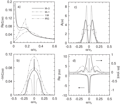
FIG. 1.: The real and imaginary parts of the self-energy (a,b), the spectral function (c), and the vertex function $\gamma$ (d) in the quasistatic approximation at $\xi\rightarrow\infty,$ $M=1$ (dot-dashed lines) and $M=3$ (solid lines) as a function of $\overline{\omega}=\omega-\varepsilon_{{\bf k}}$ for $\Delta_{0}/v_{F}=0.1,$ compared to the result of $1/M$ expansion (dotted lines) and the one-loop functional RG approach for spin-fermion model (dot-dot dashed line) for $M=3$.

For $M=1$ (charge instability case) the imaginary part of the self-energy is finite at the Fermi level [see Eq. (32)] and the spectral function has one-peak structure. It does not imply, however, the validity of the quasiparticle concept, since the real part of the self-energy has positive slope at the Fermi level, which invalidates quasiparticle picture. Note that vertex corrections are finite in this case, and, therefore, are not as important, as for $M>1.$ Since the long-range order exists for $M=1$ also at finite $T,$ these results are applicable only in a narrow critical regime near the transition temperature, but have also some implication for quantum-critical region, as discussed in Sect. IV. The behavior of $G(\omega)$, $\Sigma(\omega)$ and $\gamma(\omega)$ at $M=2$ (XY-type symmetry) is very similar to that for $M=3$, except for additional logarithmic corrections.

It is instructive to compare the results (20)-(24) for the self-energy and vertex at $\xi\rightarrow\infty$ with the corresponding results of recently proposed functional renormalization-group approach for the boson-fermion model[26]. Since the momenta integrations and frequency summations in Feynman diagrams are restricted at large $\xi$ to i$\omega_{n}=0$ and the near vicinity of $q=0$, neither frequency, nor momentum cutoff of electronic or bosonic degrees of freedom are convenient for this problem. Instead, we impose the temperature cutoff on the electronic Green function (the correlation length is kept fixed, so that the bosonic propagator does not acquire temperature dependence). We also combine this scheme with the one-particle self-consistent modification of fRG equations [27], which allows for a correct treatment of self-energy effects to one-loop order. The resulting one-loop fRG equations at $\xi\rightarrow\infty$ read

$$\frac{d\Sigma(\omega)}{d\omega} = \Delta_{0}^{2}\gamma^{2}(\omega)\frac{dG(\omega)}{d\omega}$$ (34)

$$\frac{d\gamma(\omega)}{d\omega} = -2\frac{M-2}{M}\Delta_{0}^{2}\gamma^{3}(\omega)G(\omega)\frac{dG(\omega)}{d\omega}$$ (35)

where $G(\omega)=[\omega-\Sigma(\omega)]^{-1}.$ We compare the solution of Eqs. (34) with the result of quasistatic approach (20) in Fig. 1. One can see that the one-loop fRG equations describe very accurately the perturbative regime $|\omega|\gtrsim\Delta_{0},$ but their description breaks down in the strong-coupling regime $|\omega|\lesssim\Delta_{0}.$

To study the effect of finite correlation length, we employ an ansatz for the nonuniform magnetic susceptibility

$$\chi({\bf q},0)=\frac{A}{q^{2}+\xi^{-2}}$$ (36)

Note that this ansatz neglects recently found nonanalytic corrections [21] and is, therefore, valid above the characteristic temperature $T_{X}\sim U^{2}/v_{F},$ where these corrections become important. At finite $\xi$ the quasistatic approach can be applied when static contributions to the self-energy and vertices are dominating near the Fermi level, i.e. at $\xi^{-1}\ll(T/v_{F})^{1/3},$ as discussed in the introduction. This condition is satisfied, in particular, in the RC regime.

The generalization of the quasistatic approach to the susceptibility ansatz (36) is considered in Appendix. The result (20) is to be replaced at finite $\xi$ by an integral recursion relations for the electronic self-energy $\Sigma(\omega)=\Sigma_{1}(\omega)$ and vertex $\gamma(\omega)=\gamma_{1}(\omega)$,

$$\Sigma_{j}(\omega) = \frac{\Delta_{0}^{2}c_{j}}{2\ln\xi}\int_{-\infty}^{\infty}\frac{da}{\sqrt{a^{2}+\xi^{-2}}}G_{j+1}(\omega-v_{F}a)$$ (37)

$$\gamma_{j}(\omega) = 1-\frac{\Delta_{0}^{2}r_{j}}{2\ln\xi}\int_{-\infty}^{\infty}\frac{da}{\sqrt{a^{2}+\xi^{-2}}}$$ (39)

$$\ \ \ \ \ \times\gamma_{j+1}(\omega-v_{F}a)G_{j+1}^{2}(\omega-v_{F}a)$$

where $G_{j}(\omega)=[\omega-\Sigma_{j}(\omega)]^{-1}$, $c_{j}=j/M$ (even $j$), $c_{j}=(j+M-1)/M$ (odd $j$); $r_{j}=j/(M-2)$ (even $j$), $r_{j}=(M-2)(j+M-1)/M^{2}$ (odd $j$), $G_{\infty}(\omega)=1/\omega,$ and $\gamma_{\infty}(\omega)=1.$ The most important contributions to integrals in Eqs. (37) and (39) at $\xi\rightarrow\infty$ come from a narrow vicinity of the point $a=0,$ and these equations reduce to the continuous fraction representation of the gamma-function in Eq. (20). At the same time, at finite $\xi$ the Eqs. (37) and (39) have to be solved numerically.

The results for the self-energy and the vertex are shown for different values of $\xi$ and compared with the results for $\xi\rightarrow\infty$ in Fig. 2. In agreement with previous analysis [14], the real part of the self-energy acquires a large positive slope at the Fermi level, $\partial$Re$\Sigma/\partial\varepsilon\sim T\xi^{2}.$ The $\delta$-function singularity at $\xi\rightarrow\infty$ in the imaginary part of the self-energy is replaced by the lorentian-like form of the imaginary part with $|$Im$\Sigma(0)|\sim T\xi,$ so that the quasiparticle picture is invalid at finite $\xi$ as well. With decreasing correlation length the structure of the spectral function changes from the two- to one-peak form at $\xi^{-1}\sim\Delta_{0}/v_{F}.$ Contrary to $\xi\rightarrow\infty$ limit, the vertex remains finite at finite $\xi.$

At $M=1$ the imaginary part of the self-energy, which was finite at $\xi\rightarrow\infty,$ is determined by $|$Im$\Sigma(0)|\sim\min(\Delta_{0},T\xi)$. The qp picture is violated in this case as well, since the slope of Re$\Sigma$ is positive, $\partial$Re$\Sigma/\partial\varepsilon\sim 1.$

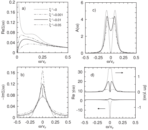
FIG. 2.: The real and imaginary parts of the self-energy (a,b), the spectral function (c), and the vertex function $\gamma$ (d) in the quasistatic approximation at $M=3$, $\Delta_{0}/v_{F}=0.1$, and different values of the correlation length.

III Two-particle properties

Now we discuss two-particle properties. First we consider static uniform spin susceptibility $\phi_{\text{ph}}.$ According to Ref. [23], this susceptibility can be expressed through the irreducible in the particle-hole channel susceptibility $\phi_{\text{ph,0}}$ via the relation

$$\phi_{\text{ph}}=\phi_{\text{ph,0}}/(1-U\phi_{\text{ph,0}})$$ (40)

which is similar to the random phase approximation result with the difference that $\phi_{\text{ph,0}}$ includes the self-energy and vertex corrections. Using the definition of the irreducible vertex, Eq. (23), we find

$$\phi_{\text{ph,0}} = \int d\varepsilon\rho_{0}(\varepsilon)\Phi(\varepsilon)$$ (41)

$$\ \Phi(\varepsilon) = -T\sum_{i\omega_{n}}\phi(i\omega_{n}-\varepsilon),\,\,\phi(z)=G^{2}(z)\gamma(z)$$ (42)

The necessary condition for the existence of a ferromagnetic instability is $\phi_{\text{ph},0}>0;$ the function $\Phi(\varepsilon)$ characterizes the relative weight of states with different energy in $\phi_{\text{ph,0}}$. The plot of the function $\phi(z)$ in the complex plane at $\xi\rightarrow\infty$ is shown in Fig. 3a (the plot of this function at finite $\xi$ looks similarly). At $\xi\rightarrow\infty$ the contribution of regions $|\omega|<\Delta_{0}$ and $|\omega|>\Delta_{0}$ to $\Phi(\varepsilon)$ have different signs and compensate each other for all $\varepsilon$, except for $|\varepsilon|<\Delta_{0},$ where $\Phi(\varepsilon)$ is maximum (Fig. 3b). Therefore, irreducible susceptibility depends on the details of the density of states only in the energy range $|\varepsilon|<\Delta_{0}$. One can see that for regular densities of states, which are not strongly suppressed in this energy range, the condition $\phi_{\text{ph,}0}>0$ can be easily fulfilled. Stronger criterium of stability of ferromagnetism $\partial^{2}\phi_{q}/\partial q^{2}<0$ is studied in detail in a forthcoming paper [22].

To investigate the static magnetic susceptibility at finite $\xi,$ we suppose that the temperature dependence of the correlation length is given by $\xi=\exp(T^{*}/T)$ where $T^{*}$ is the crossover temperature to the renormalized classical regime. The function $\Phi(\varepsilon)$ for different values of $\xi$ is shown in Fig. 3b. At not too large correlation length the energy range which contributes to $\phi_{\text{ph,0}}$ is spread to $|\varepsilon|>\Delta_{0}$ as well. At the same time, the total area under $\Phi(\varepsilon)$ changes rather weakly and, therefore, one can expect weak dependence of the irreducible susceptibility on the correlation length $\xi.$

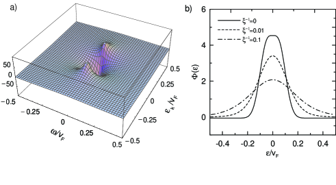
FIG. 3.: (a) The plot of the function $\phi(i\omega-\varepsilon)$ at $\xi\rightarrow\infty$ and $\Delta_{0}=0.1v_{F}$. (b) The function $\Phi(\varepsilon)$ (which determines the uniform static irreducible spin susceptibility according to Eq. (42)) at $\Delta_{0}=0.1v_{F}$, $T^{*}=0.25v_{F}$, and different values of the correlation length.

The susceptibility with respect to triplet pairing

$$\phi_{\text{pp},\text{tr}}^{a} = \sum_{{\bf kk}^{\prime}}\sum_{\sigma\sigma^{\prime}\sigma^{\prime\prime}\sigma^{\prime\prime\prime}}A_{\sigma\sigma^{\prime}}^{a}A_{\sigma^{\prime}\sigma^{\prime\prime}}^{a}\int_{0}^{\beta}d\tau$$ (44)

$$\ \ \ \ \ \times\langle T[c_{{\bf k,}\sigma}^{\dagger}(\tau)c_{-{\bf k,}\sigma^{\prime}}^{\dagger}(\tau)c_{{\bf k}^{\prime}{\bf,}\sigma^{\prime\prime}}(0)c_{-{\bf k}^{\prime}{\bf,}\sigma^{\prime\prime\prime}}(0)]\rangle$$

where $A_{\sigma\sigma^{\prime}}^{a}=(\sigma^{a}\sigma^{y})_{\sigma\sigma^{\prime}}$ can be considered in a similar way. It is convenient to represent it in the form

$$\phi_{\text{pp},\text{tr}}^{a} = T\sum_{{\bf k,}i\omega_{n}}\sum_{\sigma\sigma^{\prime}}A_{\sigma\sigma^{\prime}}^{a}\phi_{\text{pp},\text{tr}}^{a,\sigma\sigma^{\prime}}({\bf k},\omega)$$ (45)

$$\ \phi_{\text{pp},\text{tr}}^{a,\sigma\sigma^{\prime}}({\bf k},i\omega_{n}) = \sum_{{\bf k}^{\prime}{\bf,}\sigma^{\prime\prime}\sigma^{\prime\prime\prime}}\int_{0}^{\beta}d\tau\int_{0}^{\beta}d\tau^{\prime}e^{i\omega_{n}(\tau-\tau^{\prime})}$$ (48)

$$\times\langle T[c_{{\bf k,}\sigma}^{\dagger}(\tau)c_{-{\bf k,}\sigma^{\prime}}^{\dagger}(\tau^{\prime})c_{{\bf k}^{\prime}{\bf,}\sigma^{\prime\prime}}(0)$$

$$\times c_{-{\bf k}^{\prime}{\bf,}\sigma^{\prime\prime\prime}}(0)]\rangle$$

Similar to magnetic susceptibility, $\phi_{\text{pp},\text{tr}}^{a,\sigma\sigma^{\prime}}$ depends on $\varepsilon_{{\bf k}}$ and $\omega$ only and can be generally written as

$$\phi_{\text{pp},\text{tr}}^{a,\sigma\sigma^{\prime}}({\bf k},i\omega_{n}) = A_{\sigma\sigma^{\prime}}^{a}\phi_{\text{pp,tr}}(\varepsilon_{{\bf k}},i\omega)$$ (49)

$$\phi_{\text{pp,tr}}(\varepsilon_{{\bf k}},i\omega) = G(i\omega-\varepsilon_{{\bf k}})G(-i\omega_{n}-\varepsilon_{{\bf k}})\gamma_{\text{tr}}(\varepsilon_{{\bf k}},i\omega)$$ (50)

where $\gamma_{tr}(\varepsilon_{{\bf k}},i\omega)$ is the pairing vertex. At $\xi\rightarrow\infty$ we obtain

$$\phi_{\text{pp},\text{tr}}(\varepsilon_{{\bf k}},i\omega)=F(\varepsilon_{{\bf k}},\omega)+F(-\varepsilon_{{\bf k}},\omega)$$ (51)

where

$$F(\varepsilon_{{\bf k}},\omega) = \frac{\omega+(M-1)\,\varepsilon_{{\bf k}}}{2\,M\,\omega\,\overline{\omega}\varepsilon_{{\bf k}}}\,\left[1-\frac{M}{2}\left(-\frac{M\,\overline{\omega}^{2}}{2\Delta^{2}}\right)^{M/2}\right.$$ (53)

$$\left.\times e^{-\frac{M\,\overline{\omega}^{2}}{2\,\Delta^{2}}}\Gamma\left(-\frac{M}{2},-\frac{M\overline{\omega}^{2}}{2\,\Delta^{2}}\right)\right]_{\overline{\omega}=\omega-\varepsilon_{{\bf k}}}\,$$

Note that $\gamma_{tr}$ depends on $\omega$ and $\varepsilon_{{\bf k}}$ separately and $\gamma_{\text{tr}}(0,\omega)=\gamma(\omega).$ The pairing susceptibility (44) is expressed through $\phi_{\text{pp},\text{tr}}(\varepsilon_{{\bf k}},i\omega)$ by the relation

$$\phi_{\text{pp},\text{tr}} = \int d\varepsilon\rho_{0}(\varepsilon)\Phi_{\text{tr}}(\varepsilon)$$ (54)

$$\ \ \Phi_{\text{tr}}(\varepsilon) = T\sum_{i\omega_{n}}\phi_{\text{pp},\text{tr}}(\varepsilon,i\omega_{n}),$$ (55)

The function $\phi_{\text{pp},\text{tr}}(\varepsilon,i\omega),$ which characterises the contribution of different momenta and energies in the pairing susceptibility is plotted at $\xi\rightarrow\infty$ in Fig. 4a. This function is divergent at $\omega\rightarrow 0^{+},$ which signals the possibility of the triplet pairing at $T\rightarrow 0.$ At finite small $\omega$ the function $\phi_{\text{pp},\text{tr}}(\varepsilon,i\omega)$ is maximum at $\varepsilon=\pm\Delta_{0}.$ Therefore, contrary to standard BCS problem, the pairing due to the ground-state FM instability in 2D system involves particles with finite energy (with respect to the paramagnetic Fermi surface) and the momenta at the new preformed Fermi surfaces.

At finite $\xi$ the function $\phi_{\text{pp},\text{tr}}(\varepsilon_{{\bf k}},i\omega)$ is determined by the Eq. (49); the pairing vertex $\gamma_{\text{tr}}$ is obtained from the recursion relation which is similar to the recursion relation for $\gamma,$

$$\gamma_{\text{tr},j}(\varepsilon_{{\bf k}},\omega) = 1+\frac{\Delta_{0}^{2}r_{j}}{2\ln\xi}\int_{-\infty}^{\infty}\frac{da}{\sqrt{a^{2}+\xi^{-2}}}$$ (58)

$$\times\gamma_{\text{tr},j+1}(\varepsilon_{{\bf k}}-v_{F}a,\omega)G_{j+1}(\omega-\varepsilon_{{\bf k}}-v_{F}a)$$

$$\times G_{j+1}(-\omega-\varepsilon_{{\bf k}}-v_{F}a)$$

with $\gamma_{\text{tr},\infty}(\omega,\varepsilon_{{\bf k}})=1.$

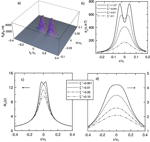
FIG. 4.: (a) The plot of the function $\phi_{\text{pp},\text{tr}}(\varepsilon,i\omega)$ at $\xi\rightarrow\infty$ and $\Delta_{0}=0.1v_{F}$ (b) The function $\phi_{\text{pp},\text{tr}}(\varepsilon,i\pi T)$ at finite $\xi$, $\Delta_{0}=0.1/5^{1/2}v_{F}$, and $T^{*}=0.05v_{F}$. (c,d) The function $\Phi_{\text{tr}}(\varepsilon)$, which determines the triplet pairing susceptibility according to Eq. (54), at the same values of $\Delta_{0}$ and $T^{*}$ as in b) (c) and at $\Delta_{0}=0.1v_{F}$, $T^{*}=0.25v_{F}$ (d).

The function $\phi_{\text{pp},\text{tr}}(\varepsilon,i\pi T)$ at different values of $\xi$ is shown in Fig. 4b. With decreasing $\xi$ the two-peak structure of $\phi_{\text{pp},\text{tr}}(\varepsilon,i\pi T)$ continuously changes to a one-peak structure at $T=T^{*}/\ln\xi\sim\Delta_{0}$. The function $\Phi_{\text{tr}}(\varepsilon)$ for two choices of $T^{*}$ and $\Delta_{0}$ and different values of the correlation length is shown in Figs. 4c,d [we rescale the value of $\Delta_{0}\propto(T^{*})^{1/2},$ as it follows from Eq. (18)]. Similar to $\phi_{\text{pp},\text{tr}}(\varepsilon,i\pi T),$ the function $\Phi_{\text{tr}}(\varepsilon)$ changes its behavior from the two-peak to a one-peak structure at $T\sim\Delta_{0}$, so that the triplet pairing fluctuations are dominating at not too large $\xi$ at the paramagnetic Fermi surface.

To clarify the role of the vertex corrections for the triplet pairing, we plot in Fig. 5 the triplet pairing vertex $\gamma_{\text{tr}}(\varepsilon,i\pi T)$ at first Matsubara frequency for the same choices of $T^{*}$ and $\Delta_{0}$ as in Fig. 4. We find that at $T^{*}\ll v_{F}$ (weakly FM ground state) and sufficiently large correlation length $\ln\xi\gg T^{*}/\Delta_{0}$ the triplet pairing vertex $\gamma_{\text{tr}}(\varepsilon,i\pi T)$ is considerably enhanced. In particular, we emphasize that the divergence of the pairing susceptibility at $\xi\rightarrow\infty$ arises solely from the vertex corrections.

The triplet pairing vertex $\gamma_{\text{tr}}(\varepsilon,i\pi T)$ in the quasistatic approach can be furthermore compared with the result $\gamma_{\text{tr}}^{E}(\varepsilon,i\pi T)$ of the approach which accounts for the self-energy corrections only (the analogue of the Eliashberg-type approach of Refs. [16, 17]). At $\xi\rightarrow\infty$ we obtain in such an approach (cf. Ref. [14])

$$\gamma_{\text{tr}}^{E}(\varepsilon,i0^{+}) = [1-(M-2)\Delta_{0}^{2}|G_{E}(\varepsilon+i0^{+})|^{2}/M]^{-1}$$ (59)

$$G_{E}(\varepsilon+i0^{+}) = [\varepsilon-\Sigma_{E}(\varepsilon+i0^{+})+i0^{+}]^{-1}$$ (60)

$$\Sigma_{E}(\varepsilon+i0^{+}) = (\varepsilon-\sqrt{\varepsilon-2\Delta_{0}}\sqrt{\varepsilon+2\Delta_{0}})/2,$$ (61)

the corresponding finite-$\xi$ result can be obtained from Eqs. (37), (58) with $c_{j}=1$ and $r_{j}=(M-2)/M$. It can be found from Eq. (61) that $\gamma_{\text{tr}}^{E}(\varepsilon,i0^{+})<M/2$ and, therefore, remains finite at $T\rightarrow 0,$ $\xi\rightarrow\infty$. At the same time, the triplet pairing vertex in the quasistatic approach is divergent in this limit, leading to the divergence of the triplet pairing susceptibility. This divergence indicates the possibility of the triplet pairing due to classical spin fluctuations, which is complementary to pairing due to quantum spin fluctuations previously studied in Refs. [16, 17]. At $\ln\xi\lesssim T^{*}/\Delta_{0}$ we find $\gamma_{\text{tr}}(\varepsilon,i\pi T)\simeq 1$ and the vertex corrections are not important. In this case, the Eliashberg-type approach of Refs. [16, 17] is justified.

Therefore, the role of the vertex corrections for the triplet pairing depends on the temperature and the value of the correlation length, at not too large correlation length the vertex corrections can be neglected, but they become crucially important at large $\xi.$

FIG. 5.: The triplet pairing vertex $\gamma_{\text{tr}}(\varepsilon,i\pi T)$ in the quasistatic approach at $\Delta_{0}=0.1/5^{1/2}v_{F}$, $T^{*}=0.05v_{F}$ (a), $\Delta_{0}=0.1v_{F}$, $T^{*}=0.25v_{F}$ (b), and different $\xi$.

IV The quantum-critical regime

As discussed previously, the static contributions to self-energy and vertices dominate over quantum contributions for sufficiently large correlation length, $\xi^{-1}\ll(T/v_{F})^{1/3}.$ Provided that this inequality is satisfied, one can apply the above consideration to the quantum-critical regime as well. As was mentioned in Sect. II, in this regime $\Delta_{0}\propto T^{1/2}\ln^{1/2}(v_{F}/T)$ becomes temperature dependent itself. The spectral properties in this case depend on the value of the exponent $\alpha$, which determines the temperature dependence of the correlation length according to $\xi\sim(T/v_{F})^{-\alpha}$. In this respect, two regimes can be distinguished: (i) $\xi^{-1}\ll\Delta_{0}/v_{F},$ i.e. $\alpha>1/2$ and (ii) $\Delta_{0}/v_{F}\lesssim\xi^{-1}\ll(T/v_{F})^{1/3},$ i.e. $1/3<\alpha\leq 1/2.$ In the regime (i) spectral functions have the two-peak structure, so that similar to the RC regime, studied in Sect. II, the Fermi-surface at finite temperatures is pre-split, while in the regime (ii) spectral functions have one-peak structure. In both regimes the real part of the self-energy has positive slope at the Fermi level $\partial$Re$\Sigma/\partial\varepsilon\sim(T/v_{F})\xi^{2}$, and the imaginary part at the Fermi level (associated with the inverse qp lifetime) is anomalously large, $|$Im$\Sigma|\sim T\xi,$ so that the qp picture is invalid. According to Millis theory [28], the temperature dependence of the correlation length in the QC regime is given by $\xi^{-1}\propto T^{1/2}\ln^{1/2}(v_{F}/T),$ and therefore this type of dependence belongs to the regime (ii).

For the charge instability case ($M=1$) the derivative of the real part of self-energy at the Fermi level is positive, but finite, $\partial$Re$\Sigma/\partial\varepsilon\sim 1,$ and the imaginary part at the Fermi level $|$Im$\Sigma|\sim\Delta_{0}\sim T^{1/2}\ln^{1/2}(v_{F}/T)$ in the regime (i) and $|$Im$\Sigma|\sim T\xi$ in the regime (ii). Note that $|$Im$\Sigma|$ in the regime (i) does not depend on the value of the exponent $\alpha$ in this case.

The triplet pairing susceptibility in the QC regime is determined by the Eq. (54). The function $\Phi_{tr}(\varepsilon)$ has a one-peak structure similar to that in the RC regime at not too large correlation length. According to the results of Sect. III, vertex corrections to the triplet pairing susceptibility are small at $T\gtrsim\Delta_{0}$ where the Eliashberg-type approach of Refs. [16, 17] is justified. The corresponding condition in the QC regime coincides, up to logarithmic corrections, with the condition of the applicability of the susceptibility ansatz (36), $T\gtrsim T_{X}$. At the same time, at $T\ll T_{X}$ triplet pairing susceptibility is substantially enhanced over its bare value and vertex corrections can not be neglected. The analysis of this case requires consideration of the nonanalytic corrections to magnetic susceptibility, which is beyond the scope of present paper. One can expect, however, that in this regime magnetic and superconducting fluctuations are strongly coupled and should be considered on the same foot.

V Conclusion

In the present paper we have studied spectral properties and the triplet pairing fluctuations in the vicinity of a FM instability. The strong FM fluctuations violate the qp concept near the Fermi level, leading to anomalously large scattering rate at the Fermi level, $|$Im$\Sigma|\sim T\xi,$ and the positive slope of the real part of the self-energy at the Fermi level, $\partial$Re$\Sigma/\partial\varepsilon\sim(T/v_{F})\xi^{2}$. Although these results coincide with the results of the second-order perturbation theory with respect to coupling of electrons with magnetic excitations [14], they take into account the self-energy and vertex corrections. Therefore, these two type of corrections almost compensate each other, as it was concluded before on the basis of $1/M$ expansion [14]. At large enough correlation length $\xi^{-1}\gg\Delta_{0}/v_{F}$ ($\Delta_{0}$ is the ground state spin splitting in the RC regime and $\Delta_{0}\propto T^{1/2}$ in the QC regime) the abovementioned features of the self-energy lead to the two-peak structure of the spectral function, which implies the quasisplitting of the Fermi surface, as proposed in Ref. [14]. The structure of the spectral function changes to a one-peak form at $\xi^{-1}\lesssim\Delta_{0}/v_{F}.$ For $M=1$ (charge instability case) the spectral function has a one-peak structure at arbitrary $\xi$. This does not restore the qp picture, however, since the slope of Re$\Sigma$ remains positive, $\partial$Re$\Sigma/\partial\varepsilon\sim 1$ and the imaginary part $|$Im$\Sigma|\sim\min(\Delta_{0},v_{F}\xi^{-1})$ is finite at low $T$.

The triplet pairing susceptibility near the FM instability is considerably enhanced at low temperatures as compared to its bare value. In the RC regime at large correlation length the triplet pairing is most strong at the newly preformed (quasi-split) Fermi-surfaces, and with increasing temperature (i.e. decreasing correlation length) the triplet pairing arises at the paramagnetic Fermi surface. The vertex corrections to the triplet pairing susceptibility are important at low enough temperatures $T\lesssim\max\{\Delta_{0},v_{F}\xi^{-1}\}.$

In the quantum critical regime, dynamic contributions with nonzero bosonic Matsubara frequency to self-energy and vertices can be neglected at low enough temperatures for $\alpha>1/3,$ where the exponent $\alpha$ describes the temperature dependence of the correlation length, $\xi\sim(T/v_{F})^{-\alpha}.$ Depending on the value of $\alpha,$ one- or two-peak structure of the spectral functions is possible, the former arising for $1/3<\alpha\leq 1/2,$ the latter for $\alpha>1/2.$ The qp picture is violated for any $\alpha<1.$ Since, however, the contributions of nonzero bosonic Matsubara frequencies are different only by power of temperature, their contribution is expected to be important for a correct quantitative description of quantum critical regime. The consideration of the triplet pairing shows that the vertex corrections in the quantum critical regime can be neglected at not too low temperatures and become non-negligible in the same temperature range $T\lesssim U^{2}/v_{F},$ where nonanalytic corrections to magnetic susceptibility become important. The consideration of this region requires an analysis of magnetic and superconducting fluctuations on the same foot, which is the subject of future investigations.

In summary, the quasistatic approximation discussed in the present paper allows for a treatment of the self-energy and vertex corrections which arise from static magnetic fluctuations. In this respect, such an approximation has some advantages over $1/M$ expansion, since it does not require $M$ to be sufficiently large. However, it can be hardly generalized to include dynamic magnetic contributions with nonzero bosonic Matsubara frequencies. Therefore, a generalization of the $1/M$ expansion, which includes these dynamic contributions, is desirable. On the other hand, the generalization of the quasistatic approach which includes the effect of van Hove singularities in the electronic spectrum could provide a possibility to describe qualitatively the properties of real low-dimensional materials.

VI Appendix. The derivation of the recursion relations at finite correlation length

In this Appendix we reconsider the extension of the quasistatic approach to 2D case when the static magnetic susceptibility has the form

$$\chi({\bf q},0)=\frac{A}{q^{2}+\xi^{-2}}$$ (62)

The early version of quasistatic approach for 1D models [18] can be directly extended to 2D case only for the factorizable form of the susceptibility (cf. Refs. [3, 19])

$$\chi({\bf q},0)=A\frac{\xi^{-1}}{q_{\|}^{2}+\xi^{-1}}\frac{\xi^{-1}}{q_{\perp}^{2}+\xi^{-1}}$$ (63)

with $q_{\|}$ and $q_{\perp}$ being the components of $q,$ parallel and perpendicular to the electron momentum ${\bf k}.$ Although the extension of quasistatic approach to the susceptibility ansatz (62) was discussed previously in Ref. [3], we argue that this extension does not treat correctly logarithmic corrections, which arise after integration of Eq. (62) over ${\bf q}.$ While these logarithmic corrections are subleading in the quantum-critical regime, they are crucially important in the RC regime, where the correlation length is exponentially large.

To discuss the way of a proper generalization of the method, we consider the contribution of a $2N$-th order diagram for the self-energy (cf. Ref. [3])

$$\Sigma^{(2N)}({\bf k},i\omega_{n}) = g^{2N}\sum_{q_{1}...q_{N}}\chi({\bf q}_{1},0)...\chi({\bf q}_{N},0)$$ (65)

$$\times\prod_{j=1}^{2N-1}\left[i\omega_{n}-\varepsilon_{{\bf k+}\sum_{\alpha=1}^{N}R_{j\alpha}{\bf q}_{\alpha}}\right]^{-1}$$

where $g=UT^{1/2}.$ The coefficients $R_{j\alpha}$ determine whether $\alpha$-th momentum variable ${\bf q}_{\alpha}$ enters $j$-th electronic Green function, see details in Ref. [3]. At large $\xi\gg 1$ the most important contribution to $\Sigma^{(2N)}$ comes from small momenta, and it is sufficient to expand the denominator of Eq. (65) in $q.$ For further convenience, we introduce new variables of integration $a_{\alpha}=q_{\alpha}\cos\theta_{\alpha}$, where $\alpha=1...N$ ($\theta_{\alpha}$ is an angle between ${\bf q}_{\alpha}$ and ${\bf k}$). The integrals over $q$ can be then calculated analytically; using the form of the susceptibility (62) we obtain

$$\Sigma^{(2N)}({\bf k}_{F},i\omega_{n}) = (Ag^{2}/4\pi)^{N}\int_{-\infty}^{\infty}\frac{da_{1}}{\sqrt{a_{1}^{2}+\xi^{-2}}}...\frac{da_{N}}{\sqrt{a_{N}^{2}+\xi^{-2}}}$$ (67)

$$\times\prod_{j=1}^{2N-1}\left[i\omega_{n}-v_{F}\sum_{\alpha=1}^{N}R_{j\alpha}a_{\alpha}\right]^{-1}$$

The corresponding result for the factorized susceptibility ansatz (63) differs by the replacement $\sqrt{a_{\alpha}^{2}+\xi^{-2}}\rightarrow\xi(a_{\alpha}^{2}+\xi^{-2})$ in the denominators of Eq. (67), $a_{\alpha}=q_{\alpha,\parallel}$ in this case.

For $|\omega|\gg v_{F}\xi^{-1}$ one can neglect $a_{\alpha}$ in the denominators of Green functions in Eq. (67) to obtain

$$\Sigma^{(2N)}({\bf k}_{F},\omega) \simeq (Ag^{2}/4\pi)^{N}\omega^{-(2N-1)}\ln^{N}(\xi\omega/v_{F}),\,\,$$ (68)

$$|\omega| \gg v_{F}\xi^{-1}$$ (69)

To find asympthotic form of the self-energy at small $|\omega|\ll v_{F}\xi^{-1}$, we shift contours of integrations in Eq. (67) to the upper half of the complex plane. The integrals are then determined by the contributions of branch cuts of square roots and

$$\Sigma^{(2N)}({\bf k}_{F},\omega) \simeq i(Ag^{2}/4\pi)^{N}\xi^{2N-1}f(\{R_{j\alpha}\}),$$ (70)

$$|\omega| \ll v_{F}\xi^{-1}.$$ (71)

where $f(\{R_{j\alpha}\})$ is some function which depends on the coeffitients $R_{j\alpha}$ only. One can see, that at $\,|\omega|\ll v_{F}\xi^{-1}$ the self-energy $\Sigma^{(2N)}({\bf k}_{F},\omega)$ does not acquire logarithmic corrections. At the same time, the approach of Ref. [3] leads to logarithmic corrections in the self-energy in both the limits, $|\omega|\gg v_{F}\xi^{-1}$ and $|\omega|\ll v_{F}\xi^{-1},$ due to an incorrect factorization of Bessel functions of sums of auxiliary variables, used in Ref. [3]. Note, that for the ansatz (63), branch cut singularities of the integrands in Eq. (67) are replaced by single poles, so that at arbitrary $|\omega|\ll v_{F}$ we obtain

$$\Sigma^{(2N)}({\bf k},\omega)\simeq(Ag^{2}/4\pi)^{N}\prod_{j=1}^{2N-1}\frac{1}{\omega-\varepsilon_{{\bf k}}+in_{j}v_{F}\xi^{-1}},$$ (72)

with $n_{j}=\sum_{\alpha=1}^{N}R_{j\alpha}$, which reproduces the result of Refs. [3, 19].

For the form of susceptibility (62) one can develop an approximate approach, which becomes exact at $|\omega|\gg v_{F}\xi^{-1}.$ Similar to Refs. [18, 19] we approximate the contribution of any diagram by the contribution of corresponding noncrossing diagram. Although the multiplicity factors are the same, as derived in Ref. [3], the expression for the corresponding noncrossing diagram is different. Indeed, substituting the dressed Green function instead of the bare one in Eq. (67) with $N=1$, and taking into account that the self-energy depends on $\omega-\varepsilon_{{\bf k}}$ only, we obtain the recursion relation

$$\Sigma_{j}(\omega) = \frac{Ag^{2}c_{j}}{4\pi}\int_{-\infty}^{\infty}\frac{da}{\sqrt{a^{2}+\xi^{-2}}}$$ (74)

$$\times\frac{1}{\omega-v_{F}a-\Sigma_{j+1}(\omega-v_{F}a)}$$

where $c_{j}=j/M$ (even $j$) and $c_{j}=(j+M-1)/M$ (odd $j$), Contrary to Ref. [3], this is an integral rather than an algebraic relation. The initial condition for Eq. (74) is $\Sigma_{\infty}(\omega)=0,$ the self-energy is given by $\Sigma(\omega)=\Sigma_{1}(\omega).$ For the vertices we obtain similarly

$$\gamma_{j}(\omega) = 1-\frac{Ag^{2}r_{j}}{4\pi}\int_{-\infty}^{\infty}\frac{da}{\sqrt{a^{2}+\xi^{-2}}}$$ (76)

$$\times\frac{\gamma_{j+1}(\omega-v_{F}a)}{[\omega-v_{F}a-\Sigma_{j+1}(\omega-v_{F}a)]^{2}}$$

$$\gamma_{\text{tr},j}(\varepsilon_{{\bf k}},\omega) = 1+\frac{Ag^{2}r_{j}}{4\pi}\int_{-\infty}^{\infty}\frac{da}{\sqrt{a^{2}+\xi^{-2}}}$$ (80)

$$\times\gamma_{\text{tr},j+1}(\varepsilon_{{\bf k}}-v_{F}a,\omega)[\omega-\varepsilon_{{\bf k}}-v_{F}a$$

$$-\Sigma_{j+1}(\omega-\varepsilon_{{\bf k}}-v_{F}a)]^{-1}[-\omega-\varepsilon_{{\bf k}}$$

$$-v_{F}a-\Sigma_{j+1}(-\omega-\varepsilon_{{\bf k}}-v_{F}a)]^{-1}$$

with $r_{j}=j/(M-2)$ (even $j$), $r_{j}=(M-2)(j+M-1)/M^{2}$ (odd $j$) and $\gamma_{\infty}(\omega)=\gamma_{\text{tr,}\infty}(\omega)=1.$

As mentioned above, for the ansatz (63) the replacement $\sqrt{a_{\alpha}^{2}+\xi^{-2}}\rightarrow a_{\alpha}^{2}\xi+\xi^{-1}$ in Eqs. (74)-(80) should be made. The integrals in the Eqs. (74) and (76) can be then evaluated analytically, leading to the recursion relations of Refs. [3, 18]. At the same time, the integrating expression of Eq. (80) is nonanalytical in both, upper and lower half-plane, and therefore can not be reduced to an algebraic form even for the factorizable susceptibility ansatz (63).

VII Acknowledgements

I am grateful to A. P. Kampf for helpful discussions and W. Metzner and V. Yu. Irkhin for many valuable comments. This work was partially supported by Grant No. 747.2003.2 (Support of Scientific Schools) from the Russian Basic Research Foundation.

REFERENCES

- [1] A. Damascelli, Z. Hussain, and Z.-X. Shen, Rev. Mod. Phys. 75, 473 (2003).
- [2] P. Monthoux, A. V. Balatsky, and D. Pines, Phys. Rev. Lett. 67, 3448 (1991); Phys. Rev. B 46, 14803 (1992).
- [3] J. Schmalian, D. Pines, and B. Stojkovic, Phys. Rev. Lett. 80, 3839 (1998); Phys. Rev. B 60, 667 (1999).
- [4] Ar. Abanov, A. V. Chubukov, and J. Schmalian, Adv. Phys. 52, 119 (2003);
- [5] J. J. Deisz, D. W. Hess, and J. W. Serene, Phys. Rev. Lett. 76, 1312 (1996); J. Altmann, W. Brenig, and A.P. Kampf, Eur. Phys. J. B 18, 429 (2000).
- [6] J. Vilk and A.-M. S. Tremblay, J. Phys. I 7, 1309 (1997); B. Kyung, Phys. Rev. B 58, 16032 (1998).
- [7] C. Huscroft, M. Jarrell, Th. Maier, S. Moukouri, and A. N. Tahvildarzadeh, Phys. Rev. Lett. 86, 139 (2001).
- [8] A. A. Katanin and A. P. Kampf, Phys. Rev. Lett. 93, 106406 (2004); D. Rohe and W. Metzner, Phys. Rev. B 71, 115116 (2005).
- [9] N. Nagaosa and P. A. Lee, Phys. Rev. Lett. 64, 2450 (1990); P. A. Lee and N. Nagaosa, Phys. Rev. B 46, 5621 (1992) .
- [10] C. Castellani, C. Di Castro, and M. Grilli, Phys. Rev. Lett. 75, 4650 (1995); C. Castellani, S. Caprara, C. Di Castro, and A. Maccarone, Nucl. Phys. B 594, 747 (2001).
- [11] W. Metzner, D. Rohe, and S. Andergassen, Phys. Rev. Lett. 91, 066402 (2003).
- [12] S. Sachdev, Quantum phase transitions, Cambridge University Press, 1999.
- [13] V. Hankevych, B. Kyung, and A.-M.S. Tremblay, Phys. Rev. B 68, 214405 (2003).
- [14] A. A. Katanin, A. P. Kampf, and V. Yu. Irkhin, Phys. Rev. B 71, 085105 (2005).
- [15] K. B. Blagoev, J. R. Engelbrecht, and K. S. Bedell, Phys. Rev. Lett. 82, 133 (1999); Z. Wang, W. Mao, and K. Bedell, Phys. Rev. Lett. 87, 257001 (2001).
- [16] A. V. Chubukov, A. M. Finkel’stein, R. Haslinger, and D. K. Morr, Phys. Rev. Lett. 90, 077002 (2003).
- [17] M. Dzero and L. P. Gor’kov, Phys. Rev. B 69, 092501 (2004).
- [18] M. V. Sadovskii, Zh. Eksp. Theor. Phys. 77, 2070 (1979) [Sov. Phys. JETP 50, 989 (1979)]
- [19] E. Z. Kuchinskii and M. V. Sadovskii, Zh. Eksp. Theor. Phys. 115, 1765 (1999) [Sov. Phys. JETP 88, 968 (1999)]; M. V. Sadovskii, Usp. Fiz. Nauk. 171, 539 (2001) [Physics-Uspekhi 44, 515 (2001)]; cond-mat/0408489 (unpublished).
- [20] P. Monthoux, Phys. Rev. B 68, 064408 (2003).
- [21] D. Belitz, T. R. Kirkpatrick, and T. Vojta, Phys. Rev. B 55, 9452 (1997); A. V. Chubukov and D. L. Maslov, Phys. Rev. B 68, 155113 (2003); A. V. Chubukov, C. Pepin, and J. Rech, Phys. Rev. Lett. 92, 147003 (2004).
- [22] P. Igoshev, A. A. Katanin, and V. Yu. Irkhin, to be published.
- [23] J. A. Hertz and D. M. Edwards, J. Phys. F 3, 2174 (1973), ibid. F 3, 2191 (1973).
- [24] A. V. Chubukov, S. Sachdev, and J. Ye, Phys. Rev. B 49, 11919 (1994).
- [25] V. Yu. Irkhin and A. A. Katanin, Phys. Rev. B 55, 12318 (1997).
- [26] F. Schuetz, L. Bartosch, and P. Kopietz, cond-mat/0409404 (unpublished).
- [27] A. A. Katanin, Phys. Rev. B 70, 115109 (2004).
- [28] A. J. Millis, Phys. Rev. B48, 7183 (1993).