Dissipating the Langevin equation in the presence of an external stochastic potential

Abstract

In the Langevin formalism, the delicate balance maintained between the fluctuations in the system and their corresponding dissipation may be upset by the presence of a secondary, space-dependent stochastic force, particularly in the low friction regime. In prior work, the latter was dissipated self-consistently through an additional uniform (mean-field) friction [Shepherd and Hernandez, J. Chem. Phys., 115, 2430-2438 (2001).] An alternative approach to ensure that equipartition is satisfied relies on the use of a space-dependent friction while ignoring nonlocal correlations. The approach is evaluated with respect to its ability to maintain constant temperature for two simple one-dimensional, stochastic potentials of mean force wherein the friction can be evaluated explicitly when there is no memory in the barriers. The use of a space-dependent friction is capable of providing qualitatively similar results to those obtained previously, but in extreme cases, deviations from equipartition may be observed due to the neglect of the memory effects present in the stochastic potentials.

I Introduction

In the theory of diffusion processes over fixed barriers, numerous studies have shown that the dissipative term in the Langevin equation is rarely constant along the reaction coordinate.Carmeli and Nitzan (1983); Straub et al. (1988); Zhu and Robinson (1988); Krishnan et al. (1992); Pollak and Berezhkovskii (1993); Straus et al. (1993); Neria and Karplus (1996); Antoniou and Schwartz (1999) A general rate theory when the friction is both space- and time-dependent has been developed to account for this phenomenon over the entire friction regime.Haynes et al. (1994, 1993); Voth (1992) One might naïvely expect that a space-dependent component must be included in the friction kernel to capture the essential dynamics of a given system. However, this is not always the case. Several groups have shown that the average dynamical properties may still be adequately described by a generalized Langevin equation with space-independent friction even when the reaction coordinate has a strong spatial dependence.Straus et al. (1993); Straub et al. (1988); Gertner et al. (1987); Krishnan et al. (1992) An analysis by Haynes and Voth concluded that the key factor is not whether the friction is space-dependent, since it generally will be, but rather how the friction varies along the reaction coordinate.Haynes and Voth (1995) In particular, they suggest that the symmetry of the space-dependent friction with respect to the barrier can be used as a metric for evaluating the role of the friction in the dynamics. Similar product and reactant states will give rise to similar (symmetric) friction components about the transition state. Perhaps surprisingly, an antisymmetric friction does not have a significant impact on the dynamics, while a symmetric friction can result in large deviations from the predictions of standard rate theories for processes with space-independent friction.Haynes and Voth (1995); Straus et al. (1993); Zhu and Robinson (1988); Straub et al. (1987); Krishnan et al. (1992); Antoniou and Schwartz (1999) Thus, the Langevin model with a uniform effective friction can often approximate the dynamics of projected variables even if the formal projection would have required a space-dependent model.

The central question explored in this work is whether a single uniform effective friction suffices even when the Langevin system is subjected to an external space-dependent stochastic potential. The behavior of a Brownian particle diffusing across various subsets of this class of potentials has been the subject of intense research.Doering and Gadoua (1992); Gammaitoni et al. (1998); Pollak et al. (1993); Talkner et al. (1999); Astumian and Moss (1998); den Broeck (1993); Reimann (1995); Bartussek et al. (1995); Porrà et al. (1994) This activity has largely been motivated by the discovery of resonant activation in which the rate of transport over a stochastic barrier exhibits a maximum as a function of the correlation time in the fluctuations of the barrier height.Doering and Gadoua (1992) However, until recently, simulations of these systems have not been performed in the low friction regime, where deviations from equipartition may occur, due to an inability to adequately describe the friction in the presence of an additional stochastic force.Shepherd and Hernandez (2001, 2002a) In previous work, the dissipation of this excess energy was achieved through a self-consistent approach in which the friction constant is renormalized iteratively until equipartition is satisfied.Shepherd and Hernandez (2001) This renormalization is approximate because it does not explicitly account for the correlations between the external stochastic forces across space and time, but rather uses a single mean friction to dissipate theses forces at times longer than their correlation times. A possible improvement to the self-consistent approach can be obtained by allowing the friction to be space-dependent while explicitly ignoring the memory in the stochastic potential, In the special case that the stochastic potential has no memory, then this treatment is exact. However, this approximation is often not justified when modeling real systems and therefore, the model potentials employed are chosen to have an exponentially decaying memory of their past states. In the most extreme cases, these correlations can result in deviations from equipartition during the course of the simulation, although the space-dependent friction dissipates such fluctuations correctly in most situations. The general conclusion appears to be that the more detailed space-dependent approach is in qualitative agreement with the self-consistent approach and hence, as in the fixed barrier case, Langevin systems with stochastic forces may be dissipated by a single (though renormalized) uniform friction.

The conclusions of this work are supported by a study of two different classes of one-dimensional problems in which the particle diffuses across a periodic array of coherent or incoherent barriers. These two cases can be specified by sinusoidal or merged-harmonic-oscillator potentials, respectively. For such simple forms of the stochastic potential, analytic expressions for the friction as a function of the spatial coordinate can readily be obtained and are presented in Sec. II. The resulting Langevin dynamics across these potentials dissipated either uniformly or through the space-dependent friction are illustrated in Sec. III.

II Langevin Model with Stochastic Potentials

An equation of motion describing the diffusion of a particle influenced by a stochastic potential of mean force can be adequately described by a phenomenological Langevin equation of the form,

$$\dot{v}=-\gamma(t)v+\xi(t)+F(x;t)\;,$$ (1)

where $F(x;t)\equiv-\nabla_{x}U(x;t)$ is an external stochastic force, and $\gamma(t)$ is the friction required to dissipate both the thermal forces and those due to the external stochastic potential. The thermal bath is described by $\xi(t)$, which is a Gaussian white noise source with time correlation given by the fluctuation-dissipation relation (FDR),

$$\langle\xi(t)\xi(t^{\prime})\rangle=2k_{\rm B}T\gamma_{\rm th}\delta(t-t^{\prime})\;.$$ (2)

In the limit that $F(x;t)=F(x;0)$ for all $t$, these equations reduce to the Langevin equation with $\gamma(t)=\gamma_{\rm th}$. Otherwise, the question remains as to what is the appropriate form of $\gamma(t)$. Two approaches for addressing this question are presented in Sections II.2 and II.3, after first describing the explicit forms of the stochastic potentials.

II.1 Stochastic Potential Representation

The space-dependent friction (SDF) that arises from the fluctuations in $F(x;t)$ can readily be evaluated analytically for two different classes of one-dimensional stochastic potentials. The first of these is a sinusoidal potential taking the general form,

$$U(x;t)=\left(E_{\rm b}+\frac{1}{2}\eta(t)\right)\left(\sin\left(\frac{\pi x}{2}\right)+1\right)\;,$$ (3)

in which the barriers fluctuate coherently with each other. The second is constructed using a series of merged harmonic oscillators (MHOs) in which each barrier is allowed to fluctuate independently (incoherently) of one another, and is specified by

$$U(x,t)=\left\{\begin{array}[]{ll}\frac{1}{2}k_{0}(x-x_{m}^{0})^{2}&\mbox{for $x_{m}^{0}<x\leq x_{m}^{-}$}\\ V_{m}^{\ddagger}+\frac{1}{2}k_{m}^{\ddagger}(x-x_{m}^{\ddagger})^{2}&\mbox{for $x_{m}^{-}<x\leq x_{m}^{+}$}\\ \frac{1}{2}k_{0}(x-x_{m+1}^{0})^{2}&\mbox{for $x_{m}^{+}<x\leq x_{m+1}^{0}$}\par\end{array}\right.\;,$$ (4)

where the $m^{th}$ well and adjacent barrier are centered at $x_{m}^{0}=-\lambda/2+m\lambda$ and $x_{m}^{\ddagger}=m\lambda$, respectively. The connection points are chosen to ensure continuity in the potential and its first derivative such that $x_{m}^{\pm}=\pm{k_{0}\lambda}/{(2k_{0}-2k_{m}^{\ddagger})}+m\lambda$. As opposed to the sinusoidal potential, the width of the MHO barriers varies stochastically in time according to the relation $k_{m}^{\ddagger}=-(k_{0}+\eta(m,t))$, which, in turn, defines the barrier height $V_{m}^{\ddagger}=-k_{0}k_{m}^{\ddagger}\lambda^{2}/(8k_{0}-8k_{m}^{\ddagger})$. The remaining parameters in the potentials are chosen such that the lattice spacing is 4 and the thermal energy of the particle is $1/6$ of the average value of the barrier heights.

The stochastic term, $\eta(t)$, is defined as an Ornstein-Uhlenbeck process governed by the following differential equation,

$$\dot{\eta}(t)=-\frac{\eta(t)}{\tau_{\rm{c}}}+\sqrt{\frac{2\sigma^{2}}{\tau_{\rm{c}}}}\zeta(t)\;,$$ (5)

with the probability distribution,

$$P\left(\eta(t)\right)=\frac{1}{\sqrt{2\pi\sigma^{2}}}\exp\left(-\frac{\eta(t)^{2}}{2\sigma^{2}}\right)\;,$$ (6)

and time correlation,

$$\langle\eta(t)\eta(t^{\prime})\rangle=\sigma^{2}\exp\left(-\frac{|t-t^{\prime}|}{\tau_{\rm{c}}}\right)\;.$$ (7)

The variance of the distribution is given by $\sigma^{2}$, $\tau_{\rm{c}}$ is the correlation time, and $\zeta(t)$ is an additional white noise source. The distribution of barriers heights for the sinusoidal potential is given directly by the distribution of $\eta(t)$, but due to the nature of the expression for the barrier heights of the MHOs, the resulting distribution for this potential takes on a more complex form that is sharper and slightly skewed compared with Eq. 6. As a result, a much smaller range of fluctuations is allowed for the MHO than the sinusoidal potential to ensure that the distribution does not become significantly non-Gaussian. More details on the exact behavior of the MHO barrier heights are provided in Ref. Shepherd and Hernandez, 2001.

II.2 Uniform Dissipation

In previous work,Shepherd and Hernandez (2001) a self-consistent procedure was developed to ensure that the evolution of the system using Eq. 1 remains in thermal equilibrium. This was accomplished through an iterative procedure in which the friction, given by the sum of the two contributions from the thermal bath and the stochastic potential, $\it{i.e.}$ $\gamma\equiv\gamma_{\rm th}+\gamma_{\rm F}$, is renormalized according to the relation,

$$\gamma^{(n+1)}=\gamma^{(n)}\left(\frac{\langle v^{2}(t)\rangle_{n}}{k_{\rm b}T}\right)\;.$$ (8)

The friction for the next iteration is determined from the value of the friction at the current step scaled by the magnitude of the deviation from equipartition seen in the dynamics until convergence is reached to within a desired accuracy. The main criticism to this approach lies in the approximation made in developing Eq. 8 in which the stochastic potential is treated as a local noise source, $\gamma_{\rm F}$, obeying a fluctuation-dissipation relation equivalent to Eq. 2. However, the stochastic potentials have memory and are therefore nonlocal in nature leading to non-vanishing cumulants at third and higher orders. These effects are included, but only in an average manner, to second order in this approach.

II.3 Space-Dependent Dissipation

An alternative approach to dissipating the external stochastic force relies on replacing the space- and time-dependent friction, $\gamma(x,t)$, by a space-dependent friction, $\gamma(x(t))$, satisfying a local FDR. Given that the size of the fluctuations in $F(x;t)$ depend on $x$ at a given $t$, a Brownian particle moving quickly across the surface will experience a series of forces whose relative magnitudes depend on the particle’s velocity. However when the the Brownian particle moves slowly, the particle will sample only the local fluctuations of the stochastic potential in the vicinity of its local position $x$. In this regime, the particle arrives at a local quasi-equilibrium which must necessarily satisfy the FDR locally. This suggests that the dissipation should not be uniform, but rather should depend on position, and therefore indirectly on time. It should be noted that while the mean-field approach described in the previous subsection is capable of including the average of the correlations between the fluctuations, the approximation made here does not account for any of the memory effects. However, in the limit that there is no memory in the external stochastic potential, the following results are exact.

The question now arises of how to explicitly describe the friction constant in the presence of an additional fluctuating force resulting from the potentials of mean force given in Eqns. 3 and  4. The friction constant must dissipate the excess energy that arises from the fluctuating forces through a local space-dependent FDR,

$$2k_{\rm B}T\gamma_{\rm c}(x;t)=\langle\delta F_{\rm c}(x;t)^{2}\rangle\;,$$ (9)

where the cumulative force is simply the sum of the thermal Gaussian noise and the stochastic force arising from the external potential, $F_{\rm c}=F_{\rm th}+F_{\rm U}$. Assuming the respective fluctuations in the bath and the potential are uncorrelated, i.e. $\langle\delta F_{\rm th}\delta F_{\rm U}\rangle=0$, then Eq. (9), reduces to

$$2k_{\rm B}T\gamma_{\rm c}(x;t)=\langle\xi(t)\xi(t^{\prime})\rangle+\langle\delta F_{\rm U}(x;t)^{2}\rangle\;,$$ (10)

The thermal fluctuations are ohmic as given in Eq. 2, and the relationship for the fluctuations in the force is $\delta F_{\rm U}(x;t)\equiv F_{\rm U}(x;t)-\langle F_{\rm U}(x;t)\rangle_{\eta}$, where the average is taken with respect to the auxiliary stochastic variable, $\eta$. The average value of the force can be determined according to the usual integrals,

$$\langle F_{\rm U}(x;t)\rangle=\frac{-\int_{-\infty}^{\infty}\!d\eta\,P(\eta)\nabla_{x}U(x;t)}{\int_{-\infty}^{\infty}\!d\eta\,P(\eta)}\;,$$ (11)

where the fluctuations in the force are governed by the stochastic Ornstein-Uhlenbeck process, $\eta$, whose probability distribution is given by Eq. 6.

The remaining steps of the derivation rely upon the specific form of the potential. As an illustration, the SDF is evaluated explicitly below for the simpler sinusoidal (coherent) stochastic potential. (The results for the incoherent MHO potential can be found in the Appendix.) The derivation begins by direct evaluation of Eq. 10 for the specific class of potentials. As remarked above, the first term reproduces the FDR, Eq. 2, for the thermal forces. Ignoring the correlation in the forces at different times, the second reduces to:

$$\langle\delta F_{\rm U}(x;t)^{2}\rangle = \frac{\pi^{2}}{4}\cos^{2}\left(\frac{\pi x}{2};t\right)\times$$ (12)

$$\int_{-\infty}^{\infty}\!d\eta\,\left(E_{\rm b}+\frac{1}{2}\eta\right)^{2}P(\eta)-$$

$$\left[\frac{\pi}{2}\cos\left(\frac{\pi x}{2};t\right)\right.\times$$

$$\left.\int_{-\infty}^{\infty}\!d\eta\,\left(E_{\rm b}+\frac{1}{2}\eta\right)P(\eta)\right]^{2}\;.$$

The Gaussian integrals are readily evaluated to yield:

$$\langle\delta F_{\rm U}(x;t)^{2}\rangle=\frac{\sigma^{2}\pi^{2}}{16}\cos^{2}(\frac{\pi x}{2};t)\;.$$ (13)

Upon substitution into Eq. 9, the explicit form of the SDF is

$$\gamma_{\rm c}(x;t)=\gamma_{\rm th}\delta(t-t^{\prime})+\frac{\sigma^{2}\pi^{2}}{32k_{\rm B}T}\cos^{2}(\frac{\pi x}{2};t)\;.$$ (14)

This is the simplest possible form for this result, and is due to the separability of the potential into a sum of deterministic and linear stochastic terms. In fact, it is easily shown that for any separable potential of the form,

$$U(x;t)=\bar{U}(x)+\eta(t)W(x)\;,$$ (15)

where $\bar{U}(x)$ is the deterministic component of the potential of mean force, then the additional friction due to the stochastic potential is given by

$$\langle\delta F_{\rm U}(x;t)^{2}\rangle=\left(\nabla_{x}W(x)\right)^{2}\int\!d\eta\,(\eta^{2}-\eta)P(\eta)\;,$$ (16)

provided the distribution is normalized. The MHO does not satisfy the condition of Eq. 15 and hence its friction correction can not be obtained by Eq. 16. The form of the friction correction for the MHO consequently contains more terms, but the requisite approximation (that the forces are uncorrelated at different times) enters the derivation in a conceptually equivalent way.

II.4 Mean First-Passage Times

The dynamics of the system were characterized by the mean first passage time (MFPT) of a particle to escape its initial minima and establish a quasi-equilibrium within another well. With periodic, stochastic potentials, this may be accomplished by defining a region of the phase space of the particle bounded by an energetic constraint.Shepherd and Hernandez (2002b) The MFPT is simply the average of a sufficient number of first passage processes into this region, with the corresponding rate given by the inverse of the MFPT. While the incorporation of a space-dependent friction in the algorithm for the numerical integration of the equations of motion would seemingly result in a dramatic increase in computational expense, the actual effort is comparable to the previous mean-field approach because the preliminary convergence procedure for the friction constant is now unnecessary.

III Results and Discussion

The analytic and numerical space-dependent components of the friction over one period of the MHO and sinusoidal potentials can be seen in the bottom panel of Figs. 1 and  2, respectively, with the numerical results averaged over 500 representative trajectories.

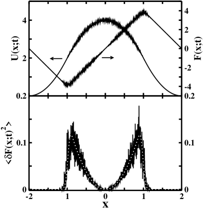
Figure 1: Representative fluctuations over one period of the MHO potential and force (top panel), and the resulting space-dependent friction (bottom panel). The numerical component in the bottom panel is displayed as the solid black line, with the analytic result, given in the Appendix, as the dotted white line. The temperature is 2/3, the variance is 0.22, and the thermal friction is 0.08.

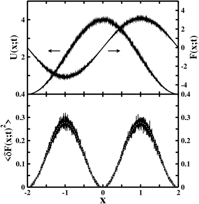
Figure 2: Representative fluctuations over one period of the sinusoidal potential and force (top panel), and the resulting space-dependent friction (bottom panel). The numerical result is displayed as the solid black line, with the analytic result, given by Eq. 14, shown as the dotted white line. The parameters used are the same as in Fig. 1.

The top panels display the fluctuations in the potential and the resulting forces that give rise to the space-dependent friction. The analytic forms of the SDF, displayed as the dotted white line, agree with the corresponding numerical results, and exact agreement is obtained upon further averaging. The fluctuations in the forces reach a maximum at approximately the midpoint between the minima and maxima, where deviations from the average force take on the largest values. The fluctuations in the potential are largest at the barriers, while the forces are zero at these locations. This leads to a vanishing contribution to the total friction from the space-dependent component at these points. In the well region, the behavior of the SDF for the sinusoidal and MHO potentials is inherently different. The SDF for the MHO is zero outside of the barrier region since the wells do not fluctuate by construction. However, the sinusoidal potential fluctuates continuously throughout leading to a friction correction along the entire reaction coordinate. Consequently, the magnitude of the friction correction in simulations employing the sinusoidal potential are slightly larger than that in those employing the MHO. But, as illustrated below, this effect does not have a dramatic effect on the resulting dynamics.

Values of the friction corrections calculated from the iterative and space-dependent approaches for the MHO and sinusoidal potentials are displayed in Table 1 with the values of the thermal friction listed in the left-most column.

	$\mbox{ }\mbox{ }\mbox{ }\mbox{ }\mbox{ }\mbox{ }\mbox{ }\mbox{ }\mbox{ }\mbox{ }\mbox{ }\mbox{ }\rm{MHO}\mbox{ }\mbox{ }\mbox{ }\mbox{ }\mbox{ }\mbox{ }\mbox{ }\mbox{ }\mbox{ }\mbox{ }\mbox{ }\mbox{ }$			$\mbox{ }\mbox{ }\mbox{ }\mbox{ }\mbox{ }\mbox{ }\mbox{ }\mbox{ }\mbox{ }\mbox{ }\mbox{ }\mbox{ }\rm{Sin}\mbox{ }\mbox{ }\mbox{ }\mbox{ }\mbox{ }\mbox{ }\mbox{ }\mbox{ }\mbox{ }\mbox{ }\mbox{ }\mbox{ }$
$\gamma_{\rm th}$	$\mbox{ }\mbox{ }\langle\gamma_{\rm{F}}\rangle_{\rm{0}}\mbox{ }\mbox{ }$	$\mbox{ }\mbox{ }\langle\gamma_{\rm{F}}\rangle_{\rm{sdf}}\mbox{ }\mbox{ }$	$\mbox{ }\mbox{ }\langle v^{2}\rangle_{\rm{sdf}}\mbox{ }\mbox{ }$	$\mbox{ }\mbox{ }\langle\gamma_{\rm{F}}\rangle_{\rm{0}}\mbox{ }\mbox{ }$	$\mbox{ }\mbox{ }\langle\gamma_{\rm{F}}\rangle_{\rm{sdf}}\mbox{ }\mbox{ }$	$\mbox{ }\mbox{ }\langle v^{2}\rangle_{\rm{sdf}}\mbox{ }\mbox{ }$
$0.08$	$0.00$	$0.01$	$0.67$	$0.00$	$0.03$	$0.69$
$0.2$	$0.00$	$0.01$	$0.67$	$0.00$	$0.03$	$0.68$
$0.4$	$0.00$	$0.01$	$0.67$	$0.01$	$0.03$	$0.67$

Table 1: The average of the friction corrections, $\gamma_{\rm F}$, calculated by the iterative self-consistent (0) and space-dependent (sdf) approaches for the MHO and sinusoidal potentials. The resulting temperatures are also included for the space-dependent friction. In all cases the temperature is 2/3 (in units of a standard temperature, $k_{\rm b}T_{0}$), the variance, $\sigma^{2}=0.22$, and the correlation time, $\tau_{\rm c}=1$.

The variance and correlation time for both potentials is 0.22 and 1, respectively. The resulting temperatures, ($k_{\rm B}T\equiv\langle v^{2}\rangle$), are also listed for the space-dependent approach. The friction correction in the self-consistent method ensures equipartition by definition, and therefore, is not listed. The magnitude of the SDF for all values of $\tau_{\rm c}$ follow accordingly; however this is the only value with respect to the given variance for which any deviation from equipartition is observed. As can be seen, both the self-consistent and space-dependent components of the total friction for each potential provide negligible contributions for this variance since the magnitude of the fluctuations in the barrier height are relatively small. Therefore the total friction is a sum of a large thermal component, and a space-dependent contribution. The slight differences in the magnitudes of the SDF for the two potentials can be attributed to the piecewise nature of the MHO potential. The particles spend most of the simulation time in the wells which do not fluctuate. A contribution to the total friction from the space-dependent term is included only when the energetically-limited particle accumulates enough energy to explore the upper portion of the MHO potential.

To further explore the accuracy of the space-dependent approach, the sinusoidal potential has been studied with a ten-fold increase in the variance from 0.22 to 2.2. The values of the friction correction from these simulations are listed in Table 2.

	$\mbox{ }\mbox{ }\mbox{ }\mbox{ }\mbox{ }\mbox{ }\mbox{ }\mbox{ }\mbox{ }\mbox{ }\mbox{ }\mbox{ }\tau_{\rm c}=10^{-1}\mbox{ }\mbox{ }\mbox{ }\mbox{ }\mbox{ }\mbox{ }\mbox{ }\mbox{ }\mbox{ }\mbox{ }\mbox{ }\mbox{ }$			$\mbox{ }\mbox{ }\mbox{ }\mbox{ }\mbox{ }\mbox{ }\mbox{ }\mbox{ }\mbox{ }\mbox{ }\mbox{ }\mbox{ }\tau_{\rm c}=10^{0}\mbox{ }\mbox{ }\mbox{ }\mbox{ }\mbox{ }\mbox{ }\mbox{ }\mbox{ }\mbox{ }\mbox{ }\mbox{ }\mbox{ }$			$\mbox{ }\mbox{ }\mbox{ }\mbox{ }\mbox{ }\mbox{ }\mbox{ }\mbox{ }\mbox{ }\mbox{ }\mbox{ }\mbox{ }\tau_{\rm c}=10^{1}\mbox{ }\mbox{ }\mbox{ }\mbox{ }\mbox{ }\mbox{ }\mbox{ }\mbox{ }\mbox{ }\mbox{ }\mbox{ }\mbox{ }$
$\gamma_{\rm th}$	$\mbox{ }\mbox{ }\langle\gamma_{\rm{F}}\rangle_{\rm{0}}\mbox{ }\mbox{ }$	$\mbox{ }\mbox{ }\langle\gamma_{\rm{F}}\rangle_{\rm{sdf}}\mbox{ }\mbox{ }$	$\mbox{ }\mbox{ }\langle v^{2}\rangle_{\rm{sdf}}\mbox{ }\mbox{ }$	$\mbox{ }\mbox{ }\langle\gamma_{\rm{F}}\rangle_{\rm{0}}\mbox{ }\mbox{ }$	$\mbox{ }\mbox{ }\langle\gamma_{\rm{F}}\rangle_{\rm{sdf}}\mbox{ }\mbox{ }$	$\mbox{ }\mbox{ }\langle v^{2}\rangle_{\rm{sdf}}\mbox{ }\mbox{ }$	$\mbox{ }\mbox{ }\langle\gamma_{\rm{F}}\rangle_{\rm{0}}\mbox{ }\mbox{ }$	$\mbox{ }\mbox{ }\langle\gamma_{\rm{F}}\rangle_{\rm{sdf}}\mbox{ }\mbox{ }$	$\mbox{ }\mbox{ }\langle v^{2}\rangle_{\rm{sdf}}\mbox{ }\mbox{ }$
$0.08$	$0.04$	$0.28$	$0.72$	$0.05$	$0.29$	$0.74$	$0.01$	$0.28$	$0.68$
$0.2$	$0.04$	$0.28$	$0.71$	$0.05$	$0.29$	$0.72$	$0.01$	$0.28$	$0.68$
$0.4$	$0.04$	$0.28$	$0.70$	$0.06$	$0.29$	$0.71$	$0.01$	$0.28$	$0.67$

Table 2: The average of the friction corrections, $\gamma_{\rm F}$, calculated by the iterative self-consistent (0) and space-dependent approaches (sdf) for the sinusoidal potential. The resulting temperatures are also included for the space-dependent friction method. The temperature is 2/3 in all cases and the variance, $\sigma^{2}=2.2$.

The displayed correlation times, $\tau_{\rm c}$, are those that exhibit the largest resonant activation. Consequently, if memory effects in the barrier heights are important in determining the friction constant, it should be manifested here. Although not shown for brevity, outside this region of the correlation time, the magnitude of the deviations from equipartition decrease rapidly, but the size of the space-dependent components remains roughly constant. Similarly, the corresponding corrections arising in the self-consistent method also approach zero. As can be seen from Table 2, the space-dependent approach results in a correction that is roughly constant for all values of the correlation time, while the iterative approach does exhibit some variation with $\tau_{\rm c}$. This is the expected result since the space-dependent friction assumes the fluctuations in the potential are local and therefore, ignores any correlation in the barrier heights. The iterative approach, however, is capable of incorporating the memory of the potential into the friction correction, but only in an average manner. As a consequence, significant deviations from equipartition may be observed when simulations are performed with a space-dependent friction that ignores the correlation effects, as illustrated by this extreme example.

Figs. 3 and  4 display the MFPTs obtained for the MHO potential with the results from the space-dependent and self-consistent approaches in the top and bottom panels, respectively.

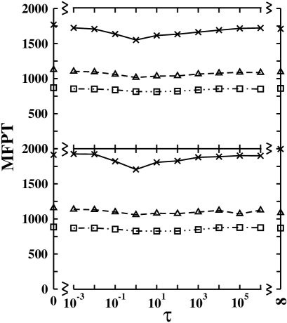
Figure 3: The mean first-passage times (MFPT) for a particle diffusing across the MHO stochastic potential are displayed for two possible scenarios of the dissipative mechanism. The top panel uses space-dependent friction, and the bottom displays the uniform friction determined by the self-consistent method. The variance for both is 0.05, and the three lines correspond to values of the thermal friction of 0.08 (solid curve with x symbols), 0.2 (dashed curve with triangles), and 0.4 (dot-dashed curve with squares). The symbols on the broken axis represent the numerically calculated MFPTs at the limits of the correlation time.

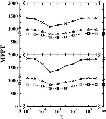
Figure 4: The mean first-passage times (MFPT) for a particle diffusing across the MHO stochastic potential are displayed for two possible scenarios of the dissipative mechanism. The parameters are the same as in Fig. 3, except the variance is 0.22.

The results in Fig. 3 have been calculated using a variance of $\sigma^{2}=0.05$, while those in Fig. 4 use $\sigma^{2}=0.22$. The corresponding results for the sinusoidal potential using a variance of 0.22 can be seen in Fig. 5.

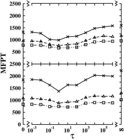
Figure 5: The mean first-passage times (MFPT) for a particle diffusing across the sinusoidal stochastic potential are displayed for two possible scenarios of the dissipative mechanism. Other than for the change from the MHO to the sinusoidal potential, the parameters are the same as in Fig. 4.

The values on the broken axis represent the numerically calculated MFPTs in the limits of correlation time, $\tau_{\rm c}$. In the zero-correlation time limit, the fluctuations in the potential are so rapid that the particle effectively experiences the average, stationary potential, from which the dynamics were calculated. In the limit of infinite correlations, fluctuations in the potential are nonexistent, and therefore the particle experiences a single realization of the potential with constant barrier heights determined by the initial value sampled from the distribution. The MFPTs displayed in Fig. 4 obtained with a larger variance alters the magnitude of the resonant activation, but influences the results for the two approaches equally. The results from the simulations with a space-dependent friction are systematically shifted to lower MFPTs as seen in all three figures. This trend is most readily explained through by the trends in Table. 1. In the low friction regime, an increase in the friction increases the corresponding rate of transport. The average space-dependent contribution is always larger than its respective mean field counterpart, and is expected to have the largest effect on the results with the smallest thermal friction. The fluctuations present along the entire reaction coordinate of the sinusoidal potential do not appear to have a dramatic effect on the dynamics. The results in Fig. 5 for the sinusoidal potential follow the same trend as those in Figs. 3 and 4 for the MHO potential indicating that the SDF approach is capable of adequately describing the fluctuations in the system. Aside from the shift, the general behavior of the MFPT is adequately reproduced by both methods, particularly at larger values of the thermal friction when the space-dependent component becomes less significant. At this level of description, each of the two approaches for constructing the friction are capable of capturing the essential dynamics of the system. However, some advantage is gained by using the self-consistent method because it ensures the system is kept at constant temperature for all values of the correlation time throughout the simulation, while the space-dependent approach may lead to deviations in extreme cases. The most significant difference between the two methods can be seen at intermediate correlation times, in which the resonant activation observed from the iterative approach is slightly more pronounced. This can particularly be seen in the MFPTs when the friction case takes on the smallest value of $\gamma_{\rm{th}}=0.08$. Since the resonant activation arises from correlations in the barrier heights, it is not surprising that simulations incorporating a friction capable of accounting for this phenomenon can have a noticeable impact on the dynamics, even if it does so only in an average manner.

IV Conclusions

The space-dependent friction arising from the presence of a secondary (external) stochastic potential in the Langevin equation has been explicitly derived for two simple classes of the stochastic potentials. The numerical results are in excellent agreement with analytic expressions describing the space-dependent friction. The resulting dynamics have been compared to those obtained using an alternate approach in which a uniform correction is calculated self-consistently. Although the latter approach does effectively include the time correlation between the barrier fluctuations at long times, the former does not in any sense. This neglect may result in deviations from equipartition in some extreme cases. However, both approaches are capable of capturing the essential dynamics of the system and lead to the now-expected resonant activation phenomenon. Consequently, the central result of this paper is that the Langevin dynamics of a particle under external stochastic potentials can be properly dissipated by a single uniform renormalized friction without loss of qualitative (and often quantitative) accuracy.

The role of the memory time in an external stochastic potential acting on a particle described by a generalized Langevin equation of motion is still an open question. In this limit, there would presumably be an interplay between the memory time of the thermal friction and that of the stochastic potential. When the latter is small compared to the former, the quasi-equilibrium condition central to this work would no longer be satisfied by the particle, and hence it is expected that a non-uniform (and time-dependent) friction correction would then be needed.

V Acknowledgments

RH gratefully acknowledges Abraham Nitzan for an insightful question whose answer became this paper. This work has been partially supported by a National Science Foundation Grant, No. NSF 02-123320. The Center for Computational Science and Technology is supported through a Shared University Research (SUR) grant from IBM and Georgia Tech. Additionally, RH is the Goizueta Foundation Junior Professor.

VI Appendix

The piecewise nature of the MHO potential results in a piecewise form for the associated SDF. Although incoherent, every barrier gives rise to the same averages, and hence the procedure needs to be carried out only over a small region defined by the closed interval, $[x_{m}^{0},x_{m}^{\ddagger}]$. The limits of integration over this region can be determined from the expression for the connection points

$$x_{m}^{-}=-\frac{k_{0}\lambda}{2k_{0}-2k_{m}^{\ddagger}}+m\lambda\;,$$ (17)

where $k_{m}^{\ddagger}=-(k_{0}+\eta(t))$. This can equivalently be expressed as

$$\eta(t)=-\frac{k_{0}\lambda}{2(x_{m}^{-}-m\lambda)}-2k_{0}\;.$$ (18)

At the top of the barrier, when $x_{m}^{-}=x_{m}^{\ddagger},~{}\mbox{$\eta(t)=\infty$}.$ In the intermediate region for arbitrary $x$,

$$\eta(t) = -\frac{k_{0}\lambda}{2(x-m\lambda)}-2k_{0}$$ (19)

$$\equiv \eta^{*}\;.$$

Otherwise, at the minimum when $x_{m}^{-}=x_{m}^{0},~{}\mbox{$\eta(t)=-k_{0}$}$.

Although it is apparent from the expression for the barrier height that the corresponding distribution is non-Gaussian, the resulting forces are Gaussian with the probability given by Eq. 6. The average force for a given $x$ is simply the weighted average of the forces when $x$ is in the respective regions, $(x_{m}^{0},x_{m}^{-})$ and $(x_{m}^{-},x_{m}^{\ddagger})$, which correspond to $\eta$ regions of $(-k_{0},\eta^{*})$ and $(\eta^{*},\infty)$. The resulting integral for the average value of $F(x;t)$ is now:

$$\langle F_{\rm U}(x;t)\rangle=\frac{\int_{-k_{0}}^{\eta^{*}}\!d\eta\,F(x)P(\eta)+\int_{\eta^{*}}^{\infty}\!d\eta\,F(x)P(\eta)}{\int_{-k_{0}}^{\infty}\!d\eta\,P(\eta)}\;.$$ (20)

Here, one must be careful in determining which portion of the force to use in the above equation. For example, when $\eta<\eta^{*}$, the majority of the force is due to the barrier portion of the potential, not the well component. The average can thus be expressed as

$$\langle F_{\rm U}(x;t)\rangle=-\int_{\eta^{*}}^{\infty}\!d\eta\,k_{0}(x-x_{m}^{0})P^{\prime}(\eta)+\int_{-k_{0}}^{\eta^{*}}\!d\eta\,(k_{0}+\eta)(x-x_{m}^{\ddagger})P^{\prime}(\eta)\;,$$ (21)

where $P^{\prime}(\eta)$ is defined through the normalization condition, $\it{i.e.}$,

$$\int_{-k_{0}}^{\eta^{*}}\!d\eta\,P^{\prime}(\eta)+\int_{\eta^{*}}^{\infty}\!d\eta\,P^{\prime}(\eta)\equiv 1\;,$$ (22)

which leads to the probability distribution

$$P^{\prime}(\eta)=\frac{2}{\sqrt{2\pi\sigma^{2}}}\frac{\exp\left({-\frac{\eta^{2}}{2\sigma^{2}}}\right)}{1+\mbox{\rm{erf}}\left(\frac{k_{0}}{\sqrt{2\sigma^{2}}}\right)}\;,$$ (23)

where $\mbox{\rm{erf}}(x)$ is the standard error function. Use of the normalization condition reduces the average force to

$$\langle F_{\rm U}(x;t)\rangle=k_{0}(x-x_{m}^{\ddagger})-[k_{0}(x-x_{m}^{0})+k_{0}(x-x_{m}^{\ddagger})]\int_{\eta^{*}}^{\infty}\!d\eta\,P^{\prime}(\eta)\mbox{}+(x-x_{m}^{\ddagger})\int_{-k_{0}}^{\eta^{*}}\!d\eta\,\eta P^{\prime}(\eta)\;.$$

The remaining integrals are readily computed; the explicit form of the average force is

$$\langle F_{\rm U}(x;t)\rangle = k_{0}(x-x_{m}^{\ddagger})-\left(k_{0}(2x-x_{m}^{0}-x_{m}^{\ddagger})\right)\left(\frac{1-\mbox{\rm{erf}}\left(\frac{\eta^{*}}{\sqrt{2\sigma^{2}}}\right)}{1+\mbox{\rm{erf}}\left(\frac{k_{0}}{\sqrt{2\sigma^{2}}}\right)}\right)$$ (24)

$$\mbox{}+(x-x_{m}^{\ddagger})\sqrt{\frac{2\sigma^{2}}{\pi}}\left[\frac{\exp\left(-\frac{k_{0}^{2}}{2\sigma^{2}}\right)-\exp\left(-\frac{(\eta^{*})^{2}}{2\sigma^{2}}\right)}{1+\mbox{\rm{erf}}\left(\frac{k_{0}}{\sqrt{2\sigma^{2}}}\right)}\right]\;.$$

The second quantity to be computed is the average of the square of the force, and the derivation follows that (above) of the average force. The limits of integration are the same and the Gaussian integrals can be calculated in the same manner. Again using the normalization requirement, the first integral is eliminated such that

$$\langle F_{\rm U}(x;t)^{2}\rangle = k_{0}^{2}(x-x_{m}^{\ddagger})^{2}+[k_{0}^{2}(x-x_{m}^{0})^{2}-k_{0}^{2}(x-x_{m}^{\ddagger})^{2}]\int_{\eta^{*}}^{\infty}\!d\eta\,P^{\prime}(\eta)$$ (25)

$$\mbox{}+2k_{0}(x-x_{m}^{\ddagger})^{2}\int_{-k_{0}}^{\eta^{*}}\!d\eta\,\eta P^{\prime}(\eta)+(x-x_{m}^{\ddagger})^{2}\int_{-k_{0}}^{\eta^{*}}\!d\eta\,\eta^{2}P^{\prime}(\eta)\;.$$

The first two integrals are the same as before, and the third can be obtained with little effort. The resulting mean squared force is

$$\langle F_{\rm U}(x;t)^{2}\rangle = k_{0}^{2}(x-x_{m}^{\ddagger})^{2}+\left(k_{0}^{2}(x-x_{m}^{0})^{2}-k_{0}^{2}(x-x_{m}^{\ddagger})^{2}\right)\left(\frac{1-\mbox{\rm{erf}}\left(\frac{\eta^{*}}{\sqrt{2\sigma^{2}}}\right)}{1+\mbox{\rm{erf}}\left(\frac{k_{0}}{\sqrt{2\sigma^{2}}}\right)}\right)$$ (26)

$$\mbox{}+\frac{4k_{0}\sigma^{2}}{\sqrt{2\pi\sigma^{2}}}(x-x_{m}^{\ddagger})^{2}\left[\frac{\exp\left(-\frac{k_{0}^{2}}{2\sigma^{2}}\right)-\exp\left(-\frac{(\eta^{*})^{2}}{2\sigma^{2}}\right)}{\left(1+\mbox{\rm{erf}}\left(\frac{k_{0}}{\sqrt{2\sigma^{2}}}\right)\right)}\right]$$

$$\mbox{}+\sigma^{2}(x-x_{m}^{\ddagger})^{2}\left[\frac{\mbox{\rm{erf}}\left(\frac{\eta^{*}}{\sqrt{2\sigma^{2}}}\right)+\mbox{\rm{erf}}\left(\frac{k_{0}}{\sqrt{2\sigma^{2}}}\right)}{1+\mbox{\rm{erf}}\left(\frac{k_{0}}{\sqrt{2\sigma^{2}}}\right)}\right]$$

$$\mbox{}-\sqrt{\frac{2\sigma^{2}}{\pi}}(x-x_{m}^{\ddagger})^{2}\left[\frac{\eta^{*}\exp\left(-\frac{(\eta^{*})^{2}}{2\sigma^{2}}\right)+k_{0}\exp\left(-\frac{k_{0}^{2}}{2\sigma^{2}}\right)}{1+\mbox{\rm{erf}}\left(\frac{k_{0}}{2\sigma^{2}}\right)}\right]\;.$$

The SDF for the MHO potential is then obtained by appropriate substitutions into Eq. 9.

References

- Carmeli and Nitzan (1983) B. Carmeli and A. Nitzan, Chem. Phys. Lett. 102, 517 (1983).
- Straub et al. (1988) J. E. Straub, M. Borkovec, and B. J. Berne, J. Chem. Phys. 89, 4833 (1988).
- Zhu and Robinson (1988) S.-B. Zhu and G. W. Robinson, J. Phys. Chem. 93, 164 (1988).
- Krishnan et al. (1992) R. Krishnan, S. Singh, and G. W. Robinson, Phys. Rev. A 45, 5408 (1992).
- Pollak and Berezhkovskii (1993) E. Pollak and A. M. Berezhkovskii, J. Chem. Phys. 99, 1344 (1993).
- Straus et al. (1993) J. B. Straus, J. M. Gomez–Llorente, and G. A. Voth, J. Chem. Phys. 98, 4082 (1993).
- Neria and Karplus (1996) E. Neria and M. Karplus, J. Chem. Phys. 105, 10812 (1996).
- Antoniou and Schwartz (1999) D. Antoniou and S. D. Schwartz, J. Chem. Phys. 110, 7359 (1999).
- Haynes et al. (1994) G. R. Haynes, G. A. Voth, and E. Pollak, J. Chem. Phys. 101, 7811 (1994).
- Haynes et al. (1993) G. R. Haynes, G. A. Voth, and E. Pollak, Chem. Phys. Lett. 207, 309 (1993).
- Voth (1992) G. A. Voth, J. Chem. Phys. 97, 5908 (1992).
- Gertner et al. (1987) B. J. Gertner, J. P. Bergsma, K. R. Wilson, S. Lee, and J. T. Hynes, J. Chem. Phys. 86, 1377 (1987).
- Haynes and Voth (1995) G. R. Haynes and G. A. Voth, J. Chem. Phys. 103, 10176 (1995).
- Straub et al. (1987) J. E. Straub, M. Borkovec, and B. J. Berne, J. Phys. Chem. 91, 4995 (1987).
- Doering and Gadoua (1992) C. R. Doering and J. C. Gadoua, Phys. Rev. Lett. 69, 2318 (1992).
- Gammaitoni et al. (1998) L. Gammaitoni, P. Hänggi, P. Jung, and F. Marchesoni, Rev. Mod. Phys. 70, 223 (1998).
- Pollak et al. (1993) E. Pollak, J. Bader, B. J. Berne, and P. Talkner, Phys. Rev. Lett. 70, 3299 (1993).
- Talkner et al. (1999) P. Talkner, E. Hershkovitz, E. Pollak, and P. Hänggi, Surf. Sci. 437, 198 (1999).
- Astumian and Moss (1998) R. Astumian and F. Moss, Chaos 8, 533 (1998).
- den Broeck (1993) C. V. den Broeck, Phys. Rev. E 47, 4579 (1993).
- Reimann (1995) P. Reimann, Phys. Rev. E 52, 1579 (1995).
- Bartussek et al. (1995) R. Bartussek, A. J. R. Madureira, and P. Hänggi, Phys. Rev. E 52, R2149 (1995).
- Porrà et al. (1994) J. M. Porrà, J. Masoliver, and K. Lindenberg, Phys. Rev. E 50, 1985 (1994).
- Shepherd and Hernandez (2001) T. Shepherd and R. Hernandez, J. Chem. Phys. 115, 2430 (2001).
- Shepherd and Hernandez (2002a) T. Shepherd and R. Hernandez, J. Phys. Chem. B 106, 8176 (2002a).
- Shepherd and Hernandez (2002b) T. Shepherd and R. Hernandez, J. Chem. Phys. 117, 9227 (2002b).