Spin Glass Phase Transition on Scale-Free Networks

Abstract

We study the Ising spin glass model on scale-free networks generated by the static model using the replica method. Based on the replica-symmetric solution, we derive the phase diagram consisting of the paramagnetic (P), ferromagnetic (F), and spin glass (SG) phases as well as the Almeida-Thouless line as functions of the degree exponent $\lambda$, the mean degree $K$, and the fraction of ferromagnetic interactions $r$. To reflect the inhomogeneity of vertices, we modify the magnetization $m$ and the spin glass order parameter $q$ with vertex-weights. The transition temperature $T_{c}$ ($T_{g}$) between the P-F (P-SG) phases and the critical behaviors of the order parameters are found analytically. When $2<\lambda<3$, $T_{c}$ and $T_{g}$ are infinite, and the system is in the F phase or the mixed phase for $r>1/2$, while it is in the SG phase at $r=1/2$. $m$ and $q$ decay as power-laws with increasing temperature with different $\lambda$-dependent exponents. When $\lambda>3$, the $T_{c}$ and $T_{g}$ are finite and related to the percolation threshold. The critical exponents associated with $m$ and $q$ depend on $\lambda$ for $3<\lambda<5$ ($3<\lambda<4$) at the P-F (P-SG) boundary.

I Introduction

Recently, considerable effort has been devoted to understanding complex systems by means of networks Strogatz01 ; Albert02 ; Dorogovtsev02a ; Newman03 . An emerging phenomenon in real-world complex networks is a scale-free (SF) behavior in the degree distribution, $P_{d}(k)\sim k^{-\lambda}$, where the degree $k$ is the number of edges connected to a given vertex and $\lambda$ is the degree exponent Barabasi99 . Due to the heterogeneity of degree, many physical problems on SF networks exhibit distinct features from those in Euclidean space. For example, the critical behavior of the ferromagnetic Ising model on SF networks exhibits an anomalous behavior depending on the degree exponent $\lambda$ Aleksiejuk01 ; Dorogovtsev02b ; Leone02 ; Bianconi02 ; herrero . While the critical behaviors are of the mean field type for $\lambda>5$, they exhibit an anomalous scaling for $3<\lambda<5$. Moreover, the magnetization, ${\bar{m}}$, decreases with increasing temperature as ${\bar{m}}\sim T^{-1/(3-\lambda)}$ for $2<\lambda<3$, and so on Dorogovtsev02b ; Leone02 . The Ising spin system on the complex networks, besides being of theoretical interest, can be used to describe various real world phenomena. For example, the two Ising spin states may represent two different opinions in a society. Depending on the interaction strength between neighbors, the overall system can be in a single or mixed opinion states, corresponding to the ferromagnetic or paramagnetic phase, respectively.

In complex systems, such a description with only ferromagnetic interactions may not be sufficient in certain circumstances. In social systems, for example, the relationship between two individuals can be friendly or unfriendly. In biological systems, two genes can respond to an external perturbation coherently or incoherently in microarray assay. For such cases, the spin glass model is then more relevant to account for such competing interactions. Recently, the spin glass problem has been studied on the small world network proposed by Watts and Strogatz Watts98 through both the replica method and the cavity method Wemmenhove04 . Since SF networks are ubiquitous in nature, here we study the spin glass model on SF networks.

The spin glass problem in the Euclidean space has been studied for a long time by various methods Binder86 ; Mezard87a ; Fischer91 ; Mydosh93 . Most of the studies for spin glasses have concentrated on regular lattices or the infinite-range interaction model on fully-connected graphs, for example, the Sherrington-Kirkpatrick (SK) model Sherrington75 . To achieve our goal here, we follow the study of the dilute Ising spin glass model with infinite-range interactions, first performed by Viana and Bray (VB) Viana85 ; Kanter87 ; Mezard87b ; Mottishaw87 ; Wong88 ; Monasson98 , because the model is equivalent to the Ising spin glass problem on the random graph proposed by Erdős and Rényi (ER) Erdos59 ; Bollobas85 . The ER random graph may be constructed as follows. The number of vertices $N$ is fixed and assumed to be sufficiently large. Each vertex $i$ $(i=1,2,\ldots,N)$ is assigned a weight $p_{i}$, which is given as $p_{i}=1/N$, independent of the index $i$ for the ER model. Two vertices $i$ and $j$ are selected with probabilities $p_{i}$ and $p_{j}$, respectively, and if $i\neq j$, they are connected with an edge unless the pair is already connected, which we call the fermionic constraint. This process is repeated $NK/2$ times. In such networks, the probability that a given pair of vertices $(i,j)$ ($i\neq j$) is not connected by an edge, denoted by $1-f_{ij}$, is given by $(1-2p_{i}p_{j})^{NK/2}\simeq\exp(-NKp_{i}p_{j})$, while the connection probability is

$$f_{ij}=1-\exp(-NKp_{i}p_{j}).$$ (1)

Since $p_{i}p_{j}=1/N^{2}$ for the ER graph, the fraction of bonds present becomes $f_{ij}\approx K/N$ and the average number of connected edges is $NK/2$. So $K$ is the mean degree, and corresponds to $p$ of Ref. Viana85 .

The SF network can be constructed through a generalization of the above to the case where the vertex-weights are given by

$$p_{i}=\frac{i^{-\mu}}{\zeta_{N}(\mu)},$$ (2)

where $\mu$ is a control parameter in the range $[0,1)$, and $\zeta_{N}(\mu)\equiv\sum_{j=1}^{N}j^{-\mu}\approx{N^{1-\mu}}/(1-\mu)$. Then the resulting network is a SF network with a power-law degree distribution, $P_{d}(k)\sim k^{-\lambda}$, with $\lambda=1+1/\mu$. The model is called the static model, where the name ‘static’ originates from the fact that the number of vertices is fixed from the beginning Goh01 . This model has the advantage that many of its theoretical quantities can be calculated analytically Lee04 . Note that since $NKp_{i}p_{j}\sim N^{2\mu-1}/(ij)^{\mu}$ for finite $K$, when $0<\mu<1/2$ ($\lambda>3$),

$$f_{ij}\approx NKp_{i}p_{j},$$ (3)

however, when $1/2<\mu<1$ ($2<\lambda<3$), $f_{ij}$ does not necessarily take the form of Eq.(3), but it is given as

$$f_{ij}\approx\left\{\begin{array}[]{lllll}1&&{\rm when}&&ij\ll N^{2-1/\mu},\\ NKp_{i}p_{j}&&{\rm when}&&ij\gg N^{2-1/\mu}.\end{array}\right.$$ (6)

This is due to the fermionic constraint that at most one edge can be attached to a given pair of vertices. The mean degree of a vertex $i$ is $NKp_{i}$ and the mean degree of the network is $K$ Lee04 .

In this work, we study the Ising spin glass model defined on the static model. In Sec.II, we introduce the Hamiltonian of the spin glass system on the static model and derive the free energy by using the replica method. We also introduce physical quantities such as the magnetization, and the spin glass order parameters in a modified form. In Sec.III, we present the replica-symmetric solutions by using the SK-type approximation, from which the phase diagram including the Almeida-Thouless line and the critical behavior of the spin glass order parameters are derived. In Sec.IV, we use the perturbative approach to derive the phase diagram and the critical behaviors of the order parameters, and compare them with those obtained from the SK method. The final section is devoted to the conclusions and discussion.

II The spin glass model

We consider the Ising-type Hamiltonian,

$$\mathcal{H}=-\sum_{(i,j)\in G}J_{ij}s_{i}s_{j}~{}~{}(s_{i}=\pm 1),$$ (7)

defined on a graph $G$ realized by the static model. $J_{ij}$ is nonzero only when the vertices $i$ and $j$ are connected in $G$. The network ensemble average for a given physical quantity $A$ is taken as

$$\langle A\rangle_{K}=\sum_{G}P_{K}(G)A(G),$$ (8)

where $P_{K}(G)$ is the probability of $G$ in the ensemble and $\langle\cdots\rangle_{K}$ the average over different graph configurations. For the static model we consider here, it is given that

$$P_{K}(G)=\prod_{(i,j)\in G}f_{ij}\prod_{(i,j)\notin G}(1-f_{ij})$$ (9)

with $f_{ij}=1-\exp(-NKp_{i}p_{j})$, $p_{i}$ being given in Eq.(2).

In the spin glass problem, the coupling strengths $\{J_{ij}\}$ are also quenched random variables. We assume in this paper that each $J_{ij}$ is given as $+J$ or $-J$ with probability $r$ and $1-r$, respectively, so that the coupling strength distribution is given as

$$P_{r}(\{J_{ij}\})=\prod_{(i,j)\in G}\Big{[}r\delta(J_{ij}-J)+(1-r)\delta(J_{ij}+J)\Big{]}.$$ (10)

The case of $r=1$ ($r=1/2$) is pure ferromagnetic (fully frustrated) one, and we consider $r$ in the range of $1/2\leq r\leq 1$ throughout this work. The average of a quantity $A$ with respect to $P_{r}(\{J_{ij}\})$ is denoted as $\langle A\rangle_{r}$. Thus the free energy is evaluated as $-\beta F=\langle\langle\ln Z\rangle_{r}\rangle_{K}$ with $Z$ being the partition function for a given distribution of $\{J_{ij}\}$ on a particular graph $G$.

In this paper, the replica method is used to evaluate the free energy, i.e., $-\beta F=\lim_{n\to 0}[\langle\langle Z^{n}\rangle_{r}\rangle_{K}-1]/n$. To proceed, we evaluate the $n$-th power of the partition function,

$$\langle\langle Z^{n}\rangle_{r}\rangle_{K} = \textrm{Tr}_{\{s^{\alpha}\}}\Big{\langle}\Big{\langle}\exp(\beta\sum_{(i,j)\in G}J_{ij}\sum_{\alpha=1}^{n}s_{i}^{\alpha}s_{j}^{\alpha})\Big{\rangle}_{r}\Big{\rangle}_{K}$$ (11)

$$= \textrm{Tr}_{\{s^{\alpha}\}}\prod_{i<j}\Big{\{}(1-f_{ij})+f_{ij}\Big{\langle}\exp(\beta J_{ij}\sum_{\alpha=1}^{n}s_{i}^{\alpha}s_{j}^{\alpha})\Big{\rangle}_{r}\Big{\}}$$

$$= \textrm{Tr}_{\{s^{\alpha}\}}\exp\Big{[}\sum_{i<j}\ln\Big{\{}1+f_{ij}\Big{(}\Big{\langle}\exp(\beta J_{ij}\sum_{\alpha=1}^{n}s_{i}^{\alpha}s_{j}^{\alpha})-1\Big{\rangle}_{r}\Big{)}\Big{\}}\Big{]},$$

where the trace $\textrm{Tr}_{\{s^{\alpha}\}}$ is taken over all replicated spins $s_{i}^{\alpha}=\pm 1$, $\alpha=1,\ldots,n$ is the replica index, and $\beta=1/T$. We mention that the disorder averages over $P_{K}(G)$ and $P_{r}(\{J_{ij}\})$ can be done simultaneously since both types of disorders are independently assigned to each edge of the fully-connected graph of order $N$. The part inside the exponential in Eq.(11) can be written in the form,

$$\sum_{i<j}\ln\Big{\{}1+f_{ij}\Big{(}\Big{\langle}\exp(\beta J_{ij}\sum_{\alpha=1}^{n}s_{i}^{\alpha}s_{j}^{\alpha})-1\Big{\rangle}_{r}\Big{)}\Big{\}} = \sum_{i<j}NKp_{i}p_{j}\Big{\langle}\exp(\beta J_{ij}\sum_{\alpha=1}^{n}s_{i}^{\alpha}s_{j}^{\alpha})-1\Big{\rangle}_{r}+R$$

where $R$ stands for the remainder which are of higher order in $K$. It is shown in APPENDIX A that for finite $K$, Eq.(LABEL:argu) is $\mathcal{O}(N)$ while $R$ is at most $\mathcal{O}(1)$ for $\lambda>3$ and $\mathcal{O}(N^{3-\lambda}\ln N)$ for $2<\lambda<3$, so that it can be neglected in the free energy calculation.

Once $R$ in Eq.(LABEL:argu) can be neglected, we can proceed as in VB Viana85 . By using the relation,

$$\Big{\langle}\exp(\beta J_{ij}\sum_{\alpha=1}^{n}s_{i}^{\alpha}s_{j}^{\alpha})\Big{\rangle}_{r}=\Big{\langle}\prod_{\alpha}\Big{[}\cosh(\beta J_{ij})(1+s_{i}^{\alpha}s_{j}^{\alpha}\tanh(\beta J_{ij}))\Big{]}\Big{\rangle}_{r},$$ (13)

in Eq.(LABEL:argu) and applying the Hubbard-Stratonovich identity, Eq.(11) is reduced to the form

$$\langle\langle Z^{n}\rangle_{r}\rangle_{K}=\int d\mathbf{q}\exp\{-Nn\beta f(\mathbf{q})\}.$$ (14)

The intensive free energy $f\{\mathbf{q}\}(\equiv F/Nn)$ in the thermodynamic limit ($N\to\infty$) then becomes

$$n\beta f\{\mathbf{q}\}=\frac{K\mathbf{T}_{1}}{2}\sum_{\alpha}q_{\alpha}^{2}+\frac{K\mathbf{T}_{2}}{2}\sum_{\alpha<\beta}q_{\alpha\beta}^{2}+\frac{K\mathbf{T}_{3}}{2}\sum_{\alpha<\beta<\gamma}q_{\alpha\beta\gamma}^{2}+\cdots-\frac{1}{N}\sum_{i}\ln\textrm{Tr}_{\{s_{i}^{\alpha}\}}\exp X_{i},$$

(15)

where

$$X_{i}=NK\mathbf{T}_{1}p_{i}\sum_{\alpha}q_{\alpha}s_{i}^{\alpha}+NK\mathbf{T}_{2}p_{i}\sum_{\alpha<\beta}q_{\alpha\beta}s_{i}^{\alpha}s_{i}^{\beta}+NK\mathbf{T}_{3}p_{i}\sum_{\alpha<\beta<\gamma}q_{\alpha\beta\gamma}s_{i}^{\alpha}s_{i}^{\beta}s_{i}^{\gamma}+\cdots,$$ (16)

and

$$\mathbf{T}_{l}(T)\equiv\langle\cosh^{n}\beta J_{ij}\tanh^{l}\beta J_{ij}\rangle_{r}\stackrel{{\scriptstyle n\to 0}}{{\longrightarrow}}[r+(-1)^{l}(1-r)]\tanh^{l}\beta J~{}~{}~{}~{}(l=1,2,\ldots).$$ (17)

$\textrm{Tr}_{\{s_{i}^{\alpha}\}}$ is the trace over the replicated spins at vertex $i$ and the $N\to\infty$ limit is to be implicitly understood to the expression $\frac{1}{N}\sum_{i}$. The elements of a set $\{\mathbf{q}\}$, $q_{\alpha}$, $q_{\alpha\beta}$, $q_{\alpha\beta\gamma}$, etc., defined as

$$q_{\alpha}=\sum_{i}p_{i}\langle s_{i}^{\alpha}\rangle_{i},~{}~{}~{}~{}q_{\alpha\beta}=\sum_{i}p_{i}\langle s_{i}^{\alpha}s_{i}^{\beta}\rangle_{i},~{}~{}~{}~{}q_{\alpha\beta\gamma}=\sum_{i}p_{i}\langle s_{i}^{\alpha}s_{i}^{\beta}s_{i}^{\gamma}\rangle_{i},~{}~{}~{}~{}\hbox{etc.}$$ (18)

are the order parameters of the spin glass system, called the magnetization, the spin glass order parameter, and so on. The average is evaluated through $\langle A\rangle_{i}\equiv\textrm{Tr}_{\{s_{i}^{\alpha}\}}A\exp X_{i}/\textrm{Tr}_{\{s_{i}^{\alpha}\}}\exp X_{i}$. Note that unlike the case of the ER random graph, the order parameters are summed with weight $\{p_{i}\}$ in Eq.(18) due to the inhomogeneity of the SF networks. For the ER case however, $p_{i}=1/N$ and it becomes that ${\bar{q}_{\alpha}}=\sum_{i}\langle s_{i}^{\alpha}\rangle_{i}/N$, ${\bar{q}_{\alpha\beta}}=\sum_{i}\langle s_{i}^{\alpha}s_{i}^{\beta}\rangle_{i}/N$, ${\bar{q}_{\alpha\beta\gamma}}=\sum_{i}\langle s_{i}^{\alpha}s_{i}^{\beta}s_{i}^{\gamma}\rangle_{i}/N$, and so on Viana85 . To distinguish, we use bar notation for the unweighted cases.

Here we consider the replica symmetry (RS) in which spins with different replica index are indistinguishable, and we invoke two methods to determine the phase boundaries of the ferromagnetic (F), paramagnetic (P) and spin glass (SG) phases and the temperature dependences of the order parameters. The first is the approach similar in spirit to SK in which higher-order terms than $q_{\alpha\beta}$ in Eqs.(15) and (16) are neglected. In this method, the remaining two order parameters as well as the Almeida-Thouless line can be obtained for all temperatures. The second is the perturbative approach used in VB. In this case, we expand the term of $\ln{\rm Tr}\exp X_{i}$ in Eq.(15) up to appropriate orders, and the order parameters $q_{\alpha}$, $q_{\alpha\beta}$, $q_{\alpha\beta\gamma}$ and $q_{\alpha\beta\gamma\delta}$ are explicitly calculated. Through the perturbative approach, we can find that the contributions by higher order terms such as $q_{\alpha\beta\gamma}$ are negligible compared with those by $q_{\alpha}$ and $q_{\alpha\beta}$ near the phase transition points. Thus, the two methods produce identical results for the phase boundaries and the same critical behaviors near the transition points for the two order parameters, $q_{\alpha}$ and $q_{\alpha\beta}$.

III The Sherrington-Kirkpatrick approach

III.1 The replica symmetric free energy

We first study the RS solution Sherrington75 and obtain the phase boundaries of P, F and SG. For simplicity, the RS magnetization and the RS spin glass order parameter are denoted as $m(=q_{\alpha})$ and $q(=q_{\alpha\beta})$, respectively, and the free energy expression Eq.(15) is truncated at the order of $q$. Then the RS free energy is rewritten as

$$n\beta f(m,q)=\frac{K\mathbf{T}_{1}}{2}nm^{2}+\frac{K\mathbf{T}_{2}}{2}\frac{n(n-1)}{2}q^{2}-\frac{1}{N}\sum_{i}\ln\mathcal{Z}_{i}$$ (19)

with

$$\mathcal{Z}_{i}=\textrm{Tr}_{\{s_{i}^{\alpha}\}}\exp\Big{\{}NK\mathbf{T}_{1}p_{i}m\sum_{\alpha}s_{i}^{\alpha}+NK\mathbf{T}_{2}p_{i}q\frac{(\sum_{\alpha}s_{i}^{\alpha})^{2}-n}{2}\Big{\}}.$$ (20)

By using the Hubbard-Stratonovich identity, ${\cal Z}_{i}$ can be rewritten as

$${\cal Z}_{i}=\exp\{-\frac{n}{2}NK\mathbf{T}_{2}p_{i}q\}\int\mathcal{D}z[2\cosh\eta_{i}(z)]^{n},$$ (21)

where $\int\mathcal{D}z\cdots\equiv\frac{1}{\sqrt{2\pi}}\int_{-\infty}^{\infty}dz~{}e^{-z^{2}/2}\cdots$ and $\eta_{i}(z)\equiv NK\mathbf{T}_{1}p_{i}m+z\sqrt{NK\mathbf{T}_{2}p_{i}q}$. Then in the limit of $n\rightarrow 0$, the RS free energy becomes

$$\beta f(m,q)=\frac{1}{2}K\mathbf{T}_{1}m^{2}+\frac{1}{2}K\mathbf{T}_{2}q-\frac{1}{4}K\mathbf{T}_{2}q^{2}-\int\mathcal{D}z\frac{1}{N}\sum_{i=1}^{N}\ln[2\cosh\eta_{i}(z)].$$ (22)

By applying $(\partial f/\partial m)=0$ and $(\partial f/\partial q)=0$ to the free energy, Eq.(22), we obtain the coupled self-consistent equations for $m$ and $q$ to be

$$m=\int\mathcal{D}z\sum_{i=1}^{N}p_{i}\tanh(NK\mathbf{T}_{1}p_{i}m+z\sqrt{NK\mathbf{T}_{2}p_{i}q}),$$ (23)

and

$$q=\int\mathcal{D}z\sum_{i=1}^{N}p_{i}\tanh^{2}(NK\mathbf{T}_{1}p_{i}m+z\sqrt{NK\mathbf{T}_{2}p_{i}q}).$$ (24)

In Eqs.(23) and (24), we can see that $q$ cannot be zero unless both $m$ and $q$ are zero, while $m$ can be zero even when $q\neq 0$ which defines the SG phase.

III.2 The phase boundaries

The P-F (P-SG) phase boundary is given as the temperature, the Curie temperature $T_{c}$ (the spin glass phase transition temperature $T_{g}$), where $m$ ($q$) starts to be nonzero. We first consider the case of $\lambda>3$. When $m$ and $q$ are small, the free energy, Eq.(22), is written as

$$\beta f(m,q) = \frac{1}{2}K\mathbf{T}_{1}(1-NK\mathbf{T}_{1}\sum_{i}p_{i}^{2})m^{2}-\frac{1}{4}K\mathbf{T}_{2}(1-NK\mathbf{T}_{2}\sum_{i}p_{i}^{2})q^{2}$$ (25)

$$+$$ higher order terms.

It is known that as $K$ increases, the static model undergoes the percolation transition at

$$K_{p}=\frac{1}{N\sum_{i}p_{i}^{2}}=\frac{(\lambda-1)(\lambda-3)}{(\lambda-2)^{2}}.$$ (26)

Since $N\sum_{i}p_{i}^{2}=(\langle k^{2}\rangle_{K}-\langle k\rangle_{K})/\langle k\rangle_{K}^{2}$ with $\langle k\rangle_{K}=K$ and $\langle k^{2}\rangle_{K}$ denoting the first and the second moments of the degree for a given mean degree $K$, respectively, Eq.(26) is equivalent to the condition $\langle k^{2}\rangle_{K}=2\langle k\rangle_{K}$ Lee04 ; molloy ; cohen . Thus one obtains that

$${\bf T}_{1}(T_{c}) = K_{p}/K~{}~{}~{}~{}\hbox{for P-F,~{}~{}~{}~{}~{}~{}and}$$ (27)

$${\bf T}_{2}(T_{g}) = K_{p}/K~{}~{}~{}~{}\hbox{for P-SG},$$ (28)

where ${\bf T}_{1}(T)=(2r-1)\tanh(J/T)$ and ${\bf T}_{2}(T)=\tanh^{2}(J/T)$. Note that when $K/K_{p}<1$, there is no solution of Eqs.(27) and (28), implying that the system is always in the P state. This is because the network has an infinite component only for $K>K_{p}$. When $r=1/2$, ${\bf T}_{1}=0$ and the phase diagram is rather simple. The P-F transition does not occur, and the system is either in P or SG phase whose boundary is given by Eq.(28).

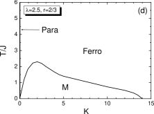
Figure 1: The phase diagram in the $(K/K_{p},T/J)$ plane for $\lambda=4.5(>3)$ with $r=1/2$ (a) and $\lambda=4.5(>3)$ with $r=2/3$ (b), and the same in the $(K,T/J)$ plane for $\lambda<3$ with $r=1/2$ (c) and $\lambda=2.5(<3)$ with $r=2/3$ (d). Note that $K_{p}=0$ for $2<\lambda<3$ in the thermodynamic limit.

FIG.1(a) is the phase diagram in the $(K/K_{p},T/J)$ plane for the fully frustrated case ($r=1/2$) for $\lambda>3$. When $1/2<r<1$, both the F phase $(m\neq 0,q\neq 0)$ and the SG phase $(m=0,q\neq 0)$ appear. FIG.1(b) is the phase diagram for a partially frustrated case with $r=2/3$ and $\lambda=4.5$, which is a prototypical case of $1/2<r<1$ and $\lambda>3$. For $K/K_{p}<1$, only the P phase appears, but for $K/K_{p}>1$, several phases exist. There exists a multicritical point $(K^{*}/K_{p},T^{*}/J)$, where the P-SG-F phases merge, which is determined to be

$$\Big{(}\frac{K^{*}}{K_{p}},\frac{T^{*}}{J}\Big{)}=\Big{(}\frac{1}{(2r-1)^{2}},\frac{1}{\tanh^{-1}(2r-1)}\Big{)}$$ (29)

by setting $\mathbf{T}_{1}(T^{*})=\mathbf{T}_{2}(T^{*})=K_{p}/K^{*}$. For $K_{p}<K<K^{*}$, the P phase goes into the SG phase, while it goes into the F phase for $K>K^{*}$ as temperature is lowered. As $r\to 1$, the multicritical point converges to $(1,0)$, indicating that only the P-F phase transition occurs. As $r\to 1/2$, it shifts to $(\infty,\infty)$, indicating that only the P-SG phase transition occurs as shown in FIG.1(a).

Besides the P, F, and SG phases, the mixed (M) phase is present, which is defined as the re-entrant SG phase with nonzero macroscopic ferromagnetic order, located below the F phase as temperature is lowered Fischer91 ; Mydosh93 . The SG-M phase boundary is determined as the vertical straight line from the multicritical point to $T/J=0$ Toulouse80 . The F-M phase boundary is determined by the so-called Almeida-Thouless (AT) line Almeida78 ,

$$(K\mathbf{T}_{2})^{-1}=\int\mathcal{D}z\sum_{i=1}^{N}Np_{i}^{2}~{}\textrm{sech}^{4}(NK{\bf T}_{1}p_{i}m+z\sqrt{NK{\bf T}_{2}p_{i}q}),$$ (30)

which is obtained easily by multiplying vertex-weights to the AT line formula of the SK model. $m$ and $q$ above are the solutions of Eqs.(23) and (24). We determine $T$ satisfying Eq.(30) numerically. The F-M boundary in FIG.1(b) exhibits a fat-tail behavior, implying that the M phase persists for large $K$. This AT line is the phase boundary between the replica symmetric phase and the replica-symmetry-broken one. Thus, Eq.(30) indicates the region where the replica-symmetric solution derived in the following sections is valid. We also check the P-SG boundary from Eq.(30), which is the same as Eq.(28).

Next we consider the case $2<\lambda<3$. In this range, $K_{p}\sim N^{-(3-\lambda)/(\lambda-1)}\to 0$ as $N\to\infty$ and consequently $T_{c}$ and $T_{g}\to\infty$. Thus the whole $(K,T/J)$ plane is covered with the ordered states. FIG.1(c) is the phase diagram for the fully frustrated case ($r=1/2$) for $\lambda<3$. The P phase appears only for $K=0$, and the SG phase is located in the region $K>0$. FIG.1(d) deals with the case of $1/2<r<1$ and $\lambda<3$. The P phase appears only at $K=0$, but for $K>0$ the F and M phases appear and the F-M boundary is given by the AT line (Eq.(30)). As $r\to 1$, the M phase disappears and only the F phase appears in the region of $K>0$.

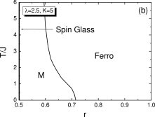
Figure 2: The phase diagram in the $(r,T/J)$ plane for $K=5$ with $\lambda=4.5(>3.0)$ (a) and $\lambda=2.5(<3.0)$ (b).

We also consider the phase diagram in the $(r,T/J)$ plane for given $\lambda$ and $K$ in FIG.2. The phase diagram is schematically similar to the one for the SK model. In the original paper of the SK model Sherrington75 , a new coupling constant $J_{0}$ of the F interactions was introduced and the ratio $J_{0}/J$ plays a similar role of the parameter $r$ here. Accordingly, the phase diagram in the $(r,T/J)$ plane here corresponds to the one in the $(J_{0}/J,T/J)$ plane in the work of the SK model. FIG.2(a) shows the phase diagram for $\lambda>3$. The formulae of the phase boundaries of P-SG and P-F are easily derived from Eqs.(27) and (28). The P-SG phase boundary is constant as $1/\tanh^{-1}\sqrt{K_{p}/K}$, independent of the parameter $r$ and the P-F phase boundary is determined as $T/J=1/\tanh^{-1}(K_{p}/K(2r-1))$. The multicritical point is determined as

$$\Big{(}r^{*},\frac{T^{*}}{J}\Big{)}=\Big{(}\frac{\sqrt{K_{p}/K}+1}{2},\frac{1}{\tanh^{-1}\sqrt{K_{p}/K}}\Big{)}.$$ (31)

The SG-M phase boundary is given by the vertical line as before. The F-M boundary is obtained from Eq.(30), finding numerically that the region of the M phase shrinks as $\lambda$ increases, and eventually it remains on the line spanning from the multicritical point to $T=0$ for a given $K$, while it exhibits a fat-tail behavior in the direction of the parameter $K$.

We plot the phase diagram in the $(r,T/J)$ plane for $\lambda<3$ with a given $K(>1)$ in FIG.2(b). Note that as $\lambda\to 3$ for a given $K$, $r^{*}$ approaches 1/2, while $T^{*}/J$ diverges to infinity. Thus, for $2<\lambda<3$, the SG phase can exist only when $r=1/2$. For $1/2<r<1$, the F and M phases exist and the F-M boundary is given by the AT line (Eq.(30)).

III.3 The SG order parameter

In the SG phase $(m=0,q\neq 0)$, the SG order parameter $q$ is determined by

$$q=\int{\cal D}z\sum_{i=1}^{N}p_{i}\tanh^{2}(z\sqrt{NK{\bf T_{2}}p_{i}q}).$$ (32)

Note that Eq.(32) is independent of $r$ but valid for $1/2\leq r<r^{*}$, $r^{*}$ being the value of $r$ at the multicritical point.

In this section, we determine the critical behavior of $q$ near the SG transition. The right hand side of Eq.(32) involves a sum of the type

$$S(y)=\frac{1}{N}\sum_{i=1}^{N}F(Np_{i}y/(1-\mu))$$ (33)

with $y=(1-\mu)K{\bf T_{2}}qz^{2}$ and $F(x)=x\tanh^{2}\sqrt{x}$. When $y$ is small in $S(y)$, a singular term $y^{\lambda-1}$ competes with other regular terms. General expressions for small $y$ expansions are derived in APPENDIX B. When Eq.(93) is used and the Gaussian integration over $z$ is performed, Eq.(32) becomes

$$q/(1-\mu)=\frac{\lambda-1}{\sqrt{\pi}}2^{\lambda-1}\Gamma(\lambda-\frac{3}{2})D(\lambda)Q^{\prime\lambda-2}-\frac{\lambda-1}{3-\lambda}Q^{\prime}+2\frac{\lambda-1}{4-\lambda}Q^{\prime 2}+\mathcal{O}(Q^{\prime 3})$$ (34)

where

$$D(\lambda)\equiv\left\{\begin{array}[]{lllll}\int_{0}^{\infty}dx~{}x^{3-2\lambda}\tanh^{2}x&&\hbox{for}&&2<\lambda<3,\\ -\int_{0}^{\infty}dx~{}x^{3-2\lambda}(x^{2}-\tanh^{2}x)&&\hbox{for}&&3<\lambda<4,\\ \end{array}\right.$$ (37)

and $Q^{\prime}=(1-\mu)K{\bf T_{2}}q=(\lambda-2)K{\bf T_{2}}q/(\lambda-1)$. Equating the right hand side of Eq.(34) with $Q^{\prime}/(1-\mu)^{2}K{\bf T_{2}}$, one sees that $Q^{\prime 3-\lambda}\sim K{\bf T_{2}}\sim T^{-2}$ for $2<\lambda<3$, $(1/K_{p}-1/K{\bf T_{2}})\sim Q^{\prime\lambda-3}$ for $3<\lambda<4$, and $(1/K_{p}-1/K{\bf T_{2}})\sim Q^{\prime}$ for $\lambda>4$. Here $K_{p}$ is given by Eq.(26) and the $\lambda$-dependent positive coefficients are neglected. Therefore, as $T\to\infty$ $(2<\lambda<3)$ or $\epsilon_{g}\equiv(T_{g}-T)/T_{g}\to 0$ $(\lambda>3)$, $q$ behaves as

$$q\sim\left\{\begin{array}[]{lllll}T^{-2(\lambda-2)/(3-\lambda)}&&{\rm for}&&2<\lambda<3,\\ \epsilon_{g}^{1/(\lambda-3)}&&{\rm for}&&3<\lambda<4,\\ \epsilon_{g}&&{\rm for}&&\lambda>4.\\ \end{array}\right.$$ (41)

When $\lambda=3$, use of Eq.(94) yields

$$q\sim T^{2}\exp(-2T^{2}/KJ^{2})~{}~{}~{}~{}{\rm as}~{}~{}T\to\infty,$$ (42)

while, when $\lambda=4$,

$$q\sim\epsilon_{g}/\ln\epsilon_{g}^{-1}~{}~{}~{}~{}{\rm as}~{}~{}\epsilon_{g}\to 0.$$ (43)

For general temperatures, $q$ can be obtained numerically from Eq.(32). The behavior of $q$ for various $\lambda$ are shown in FIG.3.

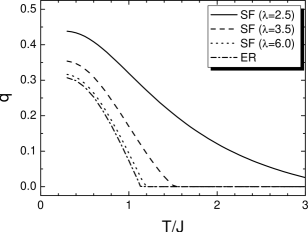
Figure 3: The behavior of $q$ in Eq.(32) for $N=5000$ and $K=2$ for $1/2\leq r<r^{*}$.

IV The perturbative approach

In this section, we use the perturbative approach to evaluate the free energy and to obtain the order parameter behaviors near the transitions. For simplicity, we use the notations defined through $Q_{\alpha}\equiv K\mathbf{T}_{1}q_{\alpha}$, $Q_{\alpha\beta}\equiv K\mathbf{T}_{2}q_{\alpha\beta}$, $Q_{\alpha\beta\gamma}\equiv K\mathbf{T}_{3}q_{\alpha\beta\gamma}$, $Q_{\alpha\beta\gamma\delta}\equiv K\mathbf{T}_{4}q_{\alpha\beta\gamma\delta}$, and so on. Let $\rm R$ represent a subset of the replica indices $\{1,2,\ldots,n\}$. Then it is convenient to denote the set $\{Q_{\alpha},Q_{\alpha\beta},\ldots\}$ as $\{Q_{\rm R}\}$. We also write $\sigma_{\rm R}\equiv\prod_{\alpha\in{\rm R}}s^{\alpha}=\pm 1$. With these notations, Eq.(16) becomes $X_{i}=\sum_{\rm R}Np_{i}Q_{\rm R}\sigma_{\rm R}$ where the sum is over all subsets of $\{1,2,\ldots,n\}$ except the null set, and

$$e^{X_{i}}=\prod_{\rm R}e^{Np_{i}Q_{\rm R}\sigma_{\rm R}}=\prod_{\rm R}\cosh Np_{i}Q_{\rm R}\prod_{\rm R}(1+\tau_{\rm R}\sigma_{\rm R})$$ (44)

with $\tau_{\rm R}\equiv\tanh Np_{i}Q_{\rm R}$. Our perturbative approach is to expand $\prod_{\rm R}(1+\tau_{\rm R}\sigma_{\rm R})$ and keep only the terms up to given order. In the ER limit $\lambda\to\infty$, we anticipate that $\tau_{\alpha}\sim\epsilon_{c}^{1/2}$, $\tau_{\alpha\beta}\sim\epsilon_{c}$, etc. from VB Viana85 , where $\epsilon_{c}\equiv(T_{c}-T)/T_{c}$ is the reduced temperature.

Using the properties that ${\rm Tr}\sigma_{\rm R}=0$, ${\rm Tr}\sigma_{\rm R}\sigma_{\rm R^{\prime}}=0$ for ${\rm R}\neq{\rm R^{\prime}}$ and so on, the first few terms relevant to our discussion below are

$$n\beta f= \frac{1}{2K\mathbf{T}_{1}}\sum_{\alpha}Q_{\alpha}^{2}+\frac{1}{2K\mathbf{T}_{2}}\sum_{\alpha<\beta}Q_{\alpha\beta}^{2}+\frac{1}{2K\mathbf{T}_{3}}\sum_{\alpha<\beta<\gamma}Q_{\alpha\beta\gamma}^{2}+\frac{1}{2K\mathbf{T}_{4}}\sum_{\alpha<\beta<\gamma<\delta}Q_{\alpha\beta\gamma\delta}^{2}$$ (45)

$$-\frac{1}{N}\sum_{i}\sum_{\rm R}\ln\cosh(Np_{i}Q_{\rm R})-\frac{1}{N}\sum_{i}\Big{[}\sum_{\alpha<\beta}\tau_{\alpha}\tau_{\beta}\tau_{\alpha\beta}+\sum_{\alpha<\beta<\gamma}\tau_{\alpha}\tau_{\beta}\tau_{\gamma}\tau_{\alpha\beta\gamma}$$

$$+\sum_{\alpha<\beta<\gamma}(\tau_{\alpha}\tau_{\beta}\tau_{\beta\gamma}\tau_{\alpha\gamma}+\tau_{\beta}\tau_{\gamma}\tau_{\alpha\beta}\tau_{\alpha\gamma}+\tau_{\gamma}\tau_{\alpha}\tau_{\alpha\beta}\tau_{\beta\gamma})+\sum_{\alpha<\beta<\gamma}\tau_{\alpha\beta}\tau_{\beta\gamma}\tau_{\alpha\gamma}$$

$$+\sum_{\alpha<\beta<\gamma<\delta}\tau_{\alpha}\tau_{\beta}\tau_{\gamma}\tau_{\delta}\tau_{\alpha\beta\gamma\delta}+\sum_{\alpha<\beta<\gamma<\delta}(\tau_{\alpha\beta}\tau_{\gamma\delta}+\tau_{\alpha\gamma}\tau_{\beta\delta}+\tau_{\alpha\delta}\tau_{\beta\gamma})\tau_{\alpha\beta\gamma\delta}$$

$$+\sum_{\alpha<\beta<\gamma<\delta}\tau_{\alpha\beta}\tau_{\beta\gamma}\tau_{\gamma\delta}\tau_{\alpha\delta}\Big{]}.$$

The result of APPENDIX B with $F(x)=\ln\cosh x$ gives

$$\frac{1}{N}\sum_{i}\ln\cosh(Np_{i}Q_{\rm R})=A(\lambda)Q_{\rm R}^{\lambda-1}+\frac{a_{2}}{2}Q_{\rm R}^{2}-\frac{a_{4}}{12}Q_{\rm R}^{4}+{\mathcal{O}}(Q_{\rm R}^{6}),$$ (46)

where

$$A(\lambda)\equiv\left\{\begin{array}[]{lllll}\frac{(\lambda-2)^{\lambda-1}}{(\lambda-1)^{\lambda-2}}\int_{0}^{\infty}dx~{}x^{-\lambda}\ln\cosh x&&\hbox{for}&&2<\lambda<3,\\ \frac{(\lambda-2)^{\lambda-1}}{(\lambda-1)^{\lambda-2}}\int_{0}^{\infty}dx~{}x^{-\lambda}\Big{(}\ln\cosh x-\frac{1}{2}x^{2}\Big{)}&&\hbox{for}&&3<\lambda<5,\\ \frac{(\lambda-2)^{\lambda-1}}{(\lambda-1)^{\lambda-2}}\int_{0}^{\infty}dx~{}x^{-\lambda}\Big{(}\ln\cosh x-\frac{1}{2}x^{2}+\frac{1}{12}x^{4}\Big{)}&&\hbox{for}&&5<\lambda<7,\end{array}\right.$$ (50)

and

$$a_{l}=(\lambda-2)^{l}/[(\lambda-1)^{l-1}(\lambda-1-l)].$$ (51)

The last sums in Eq.(45) can be represented as integrals as

$$\frac{1}{N}\sum_{i}\tau_{\rm R}\tau_{\rm R^{\prime}}\cdots=(\lambda-1)\int_{1}^{\infty}dz~{}z^{-\lambda}\tanh zQ^{\prime}_{\rm R}\tanh zQ^{\prime}_{\rm R^{\prime}}\cdots$$ (52)

with $Q^{\prime}_{\rm R}\equiv(\lambda-2)Q_{\rm R}/(\lambda-1)$.

IV.1 The replica symmetric free energy

We derive the RS solution of the order parameters up to the fourth order with the notations of $Q_{\alpha}=M$, $Q_{\alpha\beta}=Q$, $Q_{\alpha\beta\gamma}=Q_{3}$ and $Q_{\alpha\beta\gamma\delta}=Q_{4}$, respectively. Then the terms in Eq.(52) take the form of

$$\mathcal{B}_{n_{1},n_{2},n_{3},n_{4}}\equiv(\lambda-1)\int_{1}^{\infty}dz~{}z^{-\lambda}\tanh^{n_{1}}zM^{\prime}\tanh^{n_{2}}zQ^{\prime}\tanh^{n_{3}}zQ_{3}^{\prime}\tanh^{n_{4}}zQ^{\prime}_{4},$$ (53)

where $M^{\prime}\equiv(1-\mu)M=(\lambda-2)M/(\lambda-1)$, $n_{1},\ldots,n_{4}$ are integers, and other primed quantities are similarly defined.

The RS free energy $f(M,Q,Q_{3},Q_{4})$ in the limit of $n\to 0$ is then written as

$${\beta f} = \frac{b_{1}}{2}M^{2}-\frac{b_{2}}{4}Q^{2}+\frac{b_{3}}{6}Q_{3}^{2}-\frac{b_{4}}{8}Q_{4}^{2}+\frac{a_{4}}{12}M^{4}-\frac{a_{4}}{24}Q^{4}+\frac{a_{4}}{36}Q_{3}^{4}-\frac{a_{4}}{48}Q_{4}^{4}$$

$$-A(\lambda)\Big{[}M^{\lambda-1}-\frac{1}{2}Q^{\lambda-1}+\frac{1}{3}Q_{3}^{\lambda-1}-\frac{1}{4}Q_{4}^{\lambda-1}\Big{]}$$

$$+\frac{1}{2}\mathcal{B}_{2,1,0,0}-\frac{1}{3}[\mathcal{B}_{3,0,1,0}+3\mathcal{B}_{2,2,0,0}+\mathcal{B}_{0,3,0,0}]+\frac{1}{4}[\mathcal{B}_{4,0,0,1}+3\mathcal{B}_{0,2,0,1}+\mathcal{B}_{0,4,0,0}],$$

where $b_{l}\equiv(K\mathbf{T}_{l})^{-1}-a_{2}$ for $l=1,2,3$ and 4. Note that $1/a_{2}$ is nothing but $K_{p}$ for $\lambda>3$ given in Eq.(26), while it is negative for $2<\lambda<3$.

The RS solutions of $M$, $Q$, $Q_{3}$ and $Q_{4}$ are obtained by solving the self-consistent equations,

$$\partial f/\partial M=\partial f/\partial Q=\partial f/\partial Q_{3}=\partial f/\partial Q_{4}=0.$$ (55)

When $M,Q,Q_{3}$ and $Q_{4}$ are small, ${\cal B}_{n_{1},\cdots,n_{4}}$ are small. Their leading order behaviors are calculated in APPENDIX C.

The phase boundary of the P-F transition is determined as the same obtained in the SK approach. When $2<\lambda<3$, since $A(\lambda)$ is nonzero and positive, the transition temperature $T_{c}$ becomes infinity so that the system is always in the F phase when $r>1/2$. For $r=1/2$, however, $b_{1}=\infty$, and $M^{2}$ has to be zero. Then the system is in the SF phase.

IV.2 The P-F transition and the order parameters

We first consider the P-F transition. In the F phase, all the four order parameters remain nonzero. The behaviors of each order parameter within leading order are discussed below and listed in TABLE I.

order parameters	$2<\lambda<3$	$3<\lambda<4$	$4<\lambda<5$	$5<\lambda<6$	$\lambda>6$
$M$	$\sim T^{-1/(3-\lambda)}$	$\sim\epsilon_{c}^{1/(\lambda-3)}$	$\sim\epsilon_{c}^{1/(\lambda-3)}$	$\sim\epsilon_{c}^{1/2}$	$\sim\epsilon_{c}^{1/2}$
$m$	$\sim T^{-(\lambda-2)/(3-\lambda)}$	$\sim\epsilon_{c}^{1/(\lambda-3)}$	$\sim\epsilon_{c}^{1/(\lambda-3)}$	$\sim\epsilon_{c}^{1/2}$	$\sim\epsilon_{c}^{1/2}$
$Q$	$\sim T^{-(4-\lambda)/(3-\lambda)}$	$\sim\epsilon_{c}^{(\lambda-2)/(\lambda-3)}$	$\sim\epsilon_{c}^{2/(\lambda-3)}$	$\sim\epsilon_{c}^{1}$	$\sim\epsilon_{c}^{1}$
$q$	$\sim T^{-(\lambda-2)/(3-\lambda)}$	$\sim\epsilon_{c}^{(\lambda-2)/(\lambda-3)}$	$\sim\epsilon_{c}^{2/(\lambda-3)}$	$\sim\epsilon_{c}^{1}$	$\sim\epsilon_{c}^{1}$
$Q_{3}$	$\sim T^{-(7-2\lambda)/(3-\lambda)}$	$\sim\epsilon_{c}^{(\lambda-2)/(\lambda-3)}$	$\sim\epsilon_{c}^{(\lambda-2)/(\lambda-3)}$	$\sim\epsilon_{c}^{3/2}$	$\sim\epsilon_{c}^{3/2}$
$q_{3}$	$\sim T^{-(\lambda-2)/(3-\lambda)}$	$\sim\epsilon_{c}^{(\lambda-2)/(\lambda-3)}$	$\sim\epsilon_{c}^{(\lambda-2)/(\lambda-3)}$	$\sim\epsilon_{c}^{3/2}$	$\sim\epsilon_{c}^{3/2}$
$Q_{4}$	$\sim T^{-(10-3\lambda)/(3-\lambda)}$	$\sim\epsilon_{c}^{(\lambda-2)/(\lambda-3)}$	$\sim\epsilon_{c}^{(\lambda-2)/(\lambda-3)}$	$\sim\epsilon_{c}^{(\lambda-2)/2}$	$\sim\epsilon_{c}^{2}$
$q_{4}$	$\sim T^{-(\lambda-2)/(3-\lambda)}$	$\sim\epsilon_{c}^{(\lambda-2)/(\lambda-3)}$	$\sim\epsilon_{c}^{(\lambda-2)/(\lambda-3)}$	$\sim\epsilon_{c}^{(\lambda-2)/2}$	$\sim\epsilon_{c}^{2}$

Table 1: The $\lambda$-dependent critical behaviors of the four order parameters and their scaled quantities (Eq.(57)) under the P-F transition. Here $\epsilon_{c}\equiv(T_{c}-T)/T_{c}$ is the reduced temperature.

• When $2<\lambda<3$, the leading order terms in free energy $\beta f$ are

  $$\beta f \simeq -A(\lambda)M^{\lambda-1}+\frac{b_{1}}{2}M^{2}+\Big{(}\frac{1}{2}A(\lambda)-\mathcal{C}_{2,0}-\frac{1}{3}\mathcal{C}_{3,0}+\frac{1}{4}\mathcal{C}_{4,0}+\cdots\Big{)}Q^{\lambda-1}$$ (56)

  $$-\frac{b_{2}}{4}Q^{2}-\frac{1}{3}A(\lambda)Q_{3}^{\lambda-1}+\frac{b_{3}}{6}Q_{3}^{2}+\frac{1}{4}A(\lambda)Q_{4}^{\lambda-1}-\frac{b_{4}}{8}Q_{4}^{2}$$

  $$+\frac{1}{2}\mathcal{C}_{2,1}M^{\lambda-2}Q-\frac{1}{3}\mathcal{C}_{3,1}M^{\lambda-2}Q_{3}+\frac{1}{4}\mathcal{C}_{4,1}M^{\lambda-2}Q_{4}$$

  from TABLE III with $\mathcal{C}_{n,p}$ given in Eq.(101).

  By applying Eq.(55) to the free energy, we obtain the self-consistent equations for the four order parameters. Note that from the definition of $b_{l}\equiv(K{\bf T}_{l})^{-1}-a_{2}$, we find that $b_{l}\sim T^{l}$ as $T\to\infty$. All other coefficients such as $A(\lambda)$ and $\{{\cal{C}}_{n,p}\}$ are independent of $T$. From $\partial f/\partial M=0$, we obtain that $-(\lambda-1)A(\lambda)M^{\lambda-2}+b_{1}M=0$, leading to that $M\sim[(\lambda-1)A(\lambda)/b_{1}]^{1/(3-\lambda)}]\sim T^{-1/(3-\lambda)}$. From $\partial f/\partial Q=0$, we obtain that $(A(\lambda)-2{\cal{C}}_{2,0}+\cdots)(\lambda-1)Q^{\lambda-2}+\mathcal{C}_{2,1}M^{\lambda-2}-b_{2}Q=0$. Since the second term is more dominant than the first, we obtain that $Q\sim{\cal C}_{2,1}M^{\lambda-2}/b_{2}\sim T^{-(4-\lambda)/(3-\lambda)}$. Fortunately, the coefficient of $Q^{\lambda-1}$ is not needed to determine the leading order behavior of $Q$. Similarly, we obtain that $Q_{3}\sim T^{-(7-2\lambda)/(3-\lambda)}$ and $Q_{4}\sim T^{-(10-3\lambda)/(3-\lambda)}$. Subsequently, we obtain $m\sim q\sim q_{3}\sim q_{4}\sim T^{-(\lambda-2)/(3-\lambda)}$, where

  $$m=M/K{\bf T_{1}},~{}~{}q=Q/K{\bf T_{2}},~{}~{}q_{3}=Q_{3}/K{\bf T_{3}},~{}~{}\hbox{and}~{}~{}~{}q_{4}=Q_{4}/K{\bf T_{4}}.$$ (57)

  It is noteworthy that the behavior of $m$ is different from that of the unweighted magnetization, ${\bar{m}}\sim T^{-1/(3-\lambda)}$, where ${\bar{m}}=(1/N)\sum_{i}\langle s_{i}\rangle$ as previously studied in Ref.Dorogovtsev02b ; Leone02 . This is because ${\bar{m}}\sim M$ to the leading order.

• When $\lambda>3$, the transition temperature $T_{c}$ is determined by

  $$b_{1}(T_{c})=0,~{}~{}~{}\textrm{i.e.,}~{}~{}~{}a_{2}K\mathbf{T}_{1}(T_{c})=1$$ (58)

  which is the same as Eq.(27). When $3<\lambda<4$, the leading order terms in $\beta f$ are

  $$\beta f \simeq \frac{b_{1}}{2}M^{2}-A(\lambda)M^{\lambda-1}-\frac{b_{2}}{4}Q^{2}+\frac{1}{2}\mathcal{C}_{2,1}M^{\lambda-2}Q$$ (59)

  $$+\frac{b_{3}}{6}Q_{3}^{2}-\frac{1}{3}\mathcal{C}_{3,1}M^{\lambda-2}Q_{3}-\frac{b_{4}}{8}Q_{4}^{2}+\frac{1}{4}\mathcal{C}_{4,1}M^{\lambda-2}Q_{4}.$$

  Note that $A(\lambda)<0$ for $3<\lambda<5$. The most leading term is $(b_{1}/2)M^{2}$ and the transition temperature $T_{c}$ is determined by $b_{1}=0$. Just below $T_{c}$, $b_{1}<0$ and $|b_{1}|\sim{\cal O}(\epsilon_{c})$, where $\epsilon_{c}=(T_{c}-T)/T_{c}$. From $\partial f/\partial M=0$, we obtain that $-(\lambda-1)A(\lambda)M^{\lambda-2}+b_{1}M=0$, leading to that $M\sim\epsilon_{c}^{1/(\lambda-3)}$. From $\partial f/\partial Q=0$, we obtain that $\mathcal{C}_{2,1}M^{\lambda-2}-b_{2}Q=0$. Since $b_{2}$ is constant near $T_{c}$, we obtain that $Q\sim M^{\lambda-2}\sim{\epsilon_{c}}^{(\lambda-2)/(\lambda-3)}$. Similarly, it is obtained that $Q_{3}\sim M^{\lambda-2}\sim{\epsilon_{c}}^{(\lambda-2)/(\lambda-3)}$ and $Q_{4}\sim M^{\lambda-2}\sim{\epsilon_{c}}^{(\lambda-2)/(\lambda-3)}$. Unlike the case of $2<\lambda<3$, $m\sim M$, $q\sim Q$, $q_{3}\sim Q_{3}$, and $q_{4}\sim Q_{4}$. Such relations hold for all $\lambda>3$.

• When $4<\lambda<5$, the free energy is written as

  $$\beta f \simeq \frac{b_{1}}{2}M^{2}-A(\lambda)M^{\lambda-1}-\frac{b_{2}}{4}Q^{2}+\frac{a_{3}}{2}M^{2}Q$$ (60)

  $$+\frac{b_{3}}{6}Q_{3}^{2}-\frac{1}{3}\mathcal{C}_{3,1}M^{\lambda-2}Q_{3}-\frac{b_{4}}{8}Q_{4}^{2}+\frac{1}{4}\mathcal{C}_{4,1}M^{\lambda-2}Q_{4}.$$

  Following the same step as used in $3<\lambda<4$, we obtain that $M\sim\epsilon_{c}^{1/(\lambda-3)}$, $Q\sim M^{2}\sim\epsilon_{c}^{2/(\lambda-3)}$ and $Q_{3}\sim Q_{4}\sim M^{\lambda-2}\sim\epsilon_{c}^{(\lambda-2)/(\lambda-3)}$.

• When $5<\lambda<6$, the free energy is written as

  $$\beta f\simeq \frac{b_{1}}{2}M^{2}+\frac{a_{4}}{12}M^{4}-\frac{b_{2}}{4}Q^{2}+\frac{a_{3}}{2}M^{2}Q$$ (61)

  $$+\frac{b_{3}}{6}Q_{3}^{2}-\frac{a_{4}}{3}M^{3}Q_{3}-\frac{b_{4}}{8}Q_{4}^{2}+\frac{1}{4}\mathcal{C}_{4,1}M^{\lambda-2}Q_{4}.$$

  Following the same steps as before, we obtain that $M\sim\epsilon_{c}^{1/2}$, $Q\sim\epsilon_{c}$, $Q_{3}\sim\epsilon_{c}^{3/2}$, and $Q_{4}\sim\epsilon_{c}^{(\lambda-2)/2}$.

• When $\lambda>6$, the free energy is written as

  $$\beta f\simeq\frac{b_{1}}{2}M^{2}+\frac{a_{4}}{12}M^{4}-\frac{b_{2}}{4}Q^{2}+\frac{a_{3}}{2}M^{2}Q+\frac{b_{3}}{6}Q_{3}^{2}-\frac{a_{4}}{3}M^{3}Q_{3}-\frac{b_{4}}{8}Q_{4}^{2}+\frac{a_{5}}{4}M^{4}Q_{4}.$$ (62)

  Using the same step as before, it is obtained that $M\sim\epsilon_{c}^{1/2}$, $Q\sim\epsilon_{c}$, $Q_{3}\sim\epsilon_{c}^{3/2}$ and $Q_{4}\sim\epsilon_{c}^{2}$.

It is interesting to note that as $\lambda$ increases, the order parameters progressively acquire the classical mean field behavior $Q_{n}\sim\epsilon_{c}^{n/2}$ starting from the lower order ones.

IV.3 The P-SG transition and the order parameters

Here we consider the P-SG transition. In the SG phase, $M$ and $Q_{3}$ are always zero for all temperatures. Thus, the free energy becomes simpler compared with that in the F phase. Using the same method as used in the P-F transition, we obtain the P-SG transition temperature and the order parameters $Q$ and $Q_{4}$ in various region of $\lambda$, which is listed in TABLE II.

order parameters	$2<\lambda<3$	$3<\lambda<4$	$\lambda>4$
$Q$	$\sim T^{-2/(3-\lambda)}$	$\sim\epsilon_{g}^{1/(\lambda-3)}$	$\sim\epsilon_{g}^{1}$
$q$	$\sim T^{-2(\lambda-2)/(3-\lambda)}$	$\sim\epsilon_{g}^{1/(\lambda-3)}$	$\sim\epsilon_{g}^{1}$
$Q_{4}$	$\sim T^{-(8-2\lambda)/(3-\lambda)}$	$\sim\epsilon_{g}^{(\lambda-2)/(\lambda-3)}$	$\sim\epsilon_{g}^{2}$
$q_{4}$	$T^{-2(2-\lambda)/(3-\lambda)}$	$\sim\epsilon_{g}^{(\lambda-2)/(\lambda-3)}$	$\sim\epsilon_{g}^{2}$

Table 2: The $\lambda$-dependent behaviors of the two order parameters and their scaled quantities in Eq.(57) under the P-SG transition, where $\epsilon_{g}\equiv(T_{g}-T)/T_{g}$.

For more details, we first determine the P-SG phase boundary. When $2<\lambda<3$, since $A(\lambda)$, the coefficient of $Q^{\lambda-1}$ is nonzero for all $T$, the spin glass transition temperature $T_{g}$ is infinity, and no P phase exists for all $T$. When $\lambda>3$, the transition point $T_{g}$ is determined by the formula

$$b_{2}(T_{g})=0,~{}~{}\textrm{i.e.,}~{}~{}a_{2}K\mathbf{T}_{2}(T_{g})=1,~{}~{}{\rm or}~{}~{}K{\bf T}_{2}(T_{g})=K_{p}$$ (63)

which is the same as derived in the SK method. In the SG phase, the order parameter behaves as follows:

• When $2<\lambda<3$, the leading order terms of $\beta f$ read off from TABLE III with $M=Q_{3}=0$ are

  $$\beta f\simeq \Big{(}\frac{1}{2}A(\lambda)-\frac{1}{3}\mathcal{C}_{3,0}+\frac{1}{4}\mathcal{C}_{4,0}+\cdots\Big{)}Q^{\lambda-1}-\frac{b_{2}}{4}Q^{2}$$ (64)

  $$+\frac{1}{4}\Big{(}A(\lambda)Q_{4}^{\lambda-1}-\frac{b_{4}}{2}Q_{4}^{2}+3\mathcal{C}_{2,1}Q^{\lambda-2}Q_{4}\Big{)}.$$

  By applying $\partial f/\partial Q=\partial f/\partial Q_{4}=0$, we obtain that $Q\sim T^{-2/(3-\lambda)}$ and $Q_{4}\sim Q^{\lambda-2}/T^{4}\sim T^{-(8-2\lambda)/(3-\lambda)}$. Using the relation $Q=K{\bf T}_{2}q$ and $Q_{4}=K{\bf T}_{4}q_{4}$, we obtain that $q\sim q_{4}\sim T^{-2(\lambda-2)/(3-\lambda)}$. The result of $q$ is the same as the one derived through the SK method, Eq.(41). Note that the coefficient of $Q^{\lambda-1}$ in the perturbative approach is in the form of infinite series while the same is obtained in a closed form in Eq.(34).

• When $3<\lambda<4$, the free energy is

  $$\beta f\simeq-\frac{b_{2}}{4}Q^{2}+[A(\lambda)/2-\mathcal{C}_{3,0}/3+\mathcal{C}_{4,0}/4]Q^{\lambda-1}-\frac{b_{4}}{8}Q_{4}^{2}+\frac{3}{4}\mathcal{C}_{2,1}Q^{\lambda-2}Q_{4}.$$ (65)

  We note that the coefficient $b_{2}\sim-\epsilon_{g}$ with $\epsilon_{g}\equiv(T_{g}-T)/T_{g}$. Then we obtain $Q\sim\epsilon_{g}^{1/(\lambda-3)}$ Similarly, from $\partial f/\partial Q_{4}=0$, we obtain $Q_{4}\sim Q^{\lambda-2}\sim\epsilon_{g}^{(\lambda-2)/(\lambda-3)}$ with $b_{4}$ being constant.

• When $\lambda>4$, we have

  $$\beta f\simeq-\frac{b_{2}}{4}Q^{2}-\frac{a_{3}}{3}Q^{3}-\frac{b_{4}}{8}Q_{4}^{2}+\frac{3}{4}a_{3}Q^{2}Q_{4}.$$ (66)

  By following the same step above, we obtain that $Q\sim\epsilon_{g}$ and $Q_{4}\sim\epsilon_{g}^{2}$.

V conclusions

We have studied the spin glass phase transition on SF networks through the static model. The model contains generic vertex-weights in it, and edges between two vertices are connected with the probability given in Eqs. (1) and (2). The static model enables one to study the spin glass problem using the replica method by generalizing the dilute Ising spin glass model with infinite-range interactions. Here we obtained the replica-symmetric solutions through the two methods, the Sherrington-Kirkpatrick approach and the perturbative approach. We also found the phase diagram consisting of the paramagnetic (P), ferromagnetic (F), spin glass (SG), and mixed (M) phases in the space of temperature $T$, the mean degree $K$, the fraction of the ferromagnetic interactions $r$, and the degree exponent $\lambda$. The AT line was also obtained numerically. The phase diagram is shown in the $(K,T)$ and $(r,T)$ planes, which are presented in Figs. 1 and 2, respectively. The critical temperatures $T_{c}$ and $T_{g}$ for the P-F and P-SG phase transitions are simply related to the percolation threshold $K_{p}$ in Eqs.(27) and (28). We obtain the same results in the two approaches. Thus $T_{c}$ and $T_{g}$ are infinite when $2<\lambda\leq 3$. The magnetization and the spin glass order parameter are modified to account for the inhomogeneity of vertex degrees as $m=\sum_{i}p_{i}\langle s_{i}^{\alpha}\rangle_{i}$ and $q=\sum_{i}p_{i}\langle s_{i}^{\alpha}s_{i}^{\beta}\rangle_{i}$, where $p_{i}$ is the weight of vertex $i$. Such quantities depend on the degree exponent $\lambda$. When $2<\lambda<3$, due to the fact that $T_{c}=\infty$ and $T_{g}=\infty$, $m$ and $q$ decay as power-laws for large $T$ as shown in TABLES I and II, which is different from the patterns of $\bar{m}$ and $\bar{q}$, defined with $p_{i}=1/N$. When $\lambda>3$, the order parameters exhibit continuous phase transitions across $T_{c}$ and $T_{g}$, and the associated exponents depend on $\lambda$, which are listed in TABLES I and II. As $Q_{3}$, $Q_{4},\ldots$ are of higher orders, the SK approach in Sec. III, and the perturbative one in Sec. IV give the identical results for $m$ and $q$ to the leading order. We find the critical exponents for the P/SG transition are non-classical in the range $3<\lambda<4$, corresponding to $3<\lambda<5$ for the P/F one Dorogovtsev02b . We have not presented our results at integer values of $\lambda$ in Section IV for simplicity. At the borderline cases of $\lambda$, the logarithmic corrections as given in Eqs. (94), (98) and (102) should be considered explicitly. We mention that the finite-size effect is an important issue especially for $2<\lambda\leq 3$ which we leave for a further study.

It is noteworthy that the method we developed here can be applied to other problems in equilibrium statistical physics on SF networks. A novelty in this approach is that one needs not rely on the local treelike structure of SF networks used e.g. in Dorogovtsev02b . The result of the phase diagram and the behavior of the order parameters may be helpful in understanding emerging patterns in various systems with competing interactions such as social or biological systems. For example, in the region $2<\lambda\leq 3$ where most real-world SF networks belong, it is known that the structural characteristic of the network is so dominant that homogeneously interacting systems are in the ordered state for all temperatures. Our result shows that it is also the case even when there are competing interactions. Also for $2<\lambda\leq 3$, the fact that a slight dominance of cooperative interactions ($r\gtrsim 1/2$) drives the system into the ferromagnetically ordered or the mixed state suggests that most social and biological systems would be driven into the majority state (ferromagnetic or mixed state) at equilibrium. While the current study is meaningful as a first step of understanding thermodynamic property of the systems with competing interactions, further studies have to be followed towards real-world systems where the signs of interactions may be correlated with the degrees of vertices, or the interaction signs may change with time as in the prisoner’s dilemma problem.

While preparing this manuscript, we have learned of a recent preprint by Mooij and Kappen Mooij04 , which addressed the same issue. They used the Bethe approximation to obtain a criterion for $T_{g}$ and applied it to the $\lambda=\infty$ and $\lambda=3$ cases numerically. Our work gives analytic results for $T_{g}$ as well as physical ones such as the phase diagram and the behaviors of the order parameters, which depend on the degree exponent.

Appendix A Evaluation of the remainder

In this APPENDIX A, we show that

$$\sum_{i<j}\ln(1+f_{ij}S_{ij})=\sum_{i<j}NKp_{i}p_{j}S_{ij}+R$$ (67)

with $R<{\cal{O}}(N^{3-\lambda}\ln N)$ for $2<\lambda<3$, $R<{\cal{O}}((\ln N)^{2})$ for $\lambda=3$ and $R<{\cal{O}}(1)$ for $\lambda>3$. Here $S_{ij}=\langle\exp(\beta J_{ij}\sum_{\alpha=1}^{n}s_{i}^{\alpha}s_{j}^{\alpha})-1\rangle_{r}$ is a quantity independent of the system size $N$. To do so, we expand the logarithm on the left hand side of Eq.(67) to write it as

$$\sum_{i<j}\ln(1+f_{ij}S_{ij})=\sum_{i<j}NKp_{i}p_{j}S_{ij}+\sum_{i<j}(f_{ij}-NKp_{i}p_{j})S_{ij}+\sum_{n=2}^{\infty}\frac{(-1)^{n+1}}{n}\sum_{i<j}f_{ij}^{n}S_{ij}^{n}$$ (68)

and show that the positive quantities defined by

$$R^{\prime}\equiv|\sum_{i<j}(NKp_{i}p_{j}-f_{ij})S_{ij}|$$ (69)

and

$$R_{n}\equiv|\sum_{i<j}f_{ij}^{n}S_{ij}^{n}|$$ (70)

($n\geq 2$) are all bounded above by ${\sl{o}}(N)$ quantities.

First let us consider $R^{\prime}$. Since $S_{ij}$ are independent of $N$, we replace $S_{ij}$ by their maximum value $S_{\rm max}\equiv\max_{i<j}|S_{ij}|$ to get

$$R^{\prime}\leq S_{\rm max}\sum_{i<j}G_{1}(NKp_{i}p_{j})\leq\frac{S_{\rm max}}{2}[{\sum_{i,j}G_{1}(NKp_{i}p_{j})-G_{1}(NKp_{1}^{2})}],$$ (71)

where

$$G_{1}(x)\equiv x-1+e^{-x}.$$ (72)

Here we have added $i=j$ terms for $i\geq 2$ on the right hand side of Eq.(71) for convenience. Since $G_{1}(x)$ is monotone increasing for $x>0$, the summands in Eq.(71) decrease as $i$ and $j$ increase.

We utilize the fact that, for a monotone decreasing continuous function $F(x)$, a finite sum is bounded above by an integral as

$$\sum_{i=1}^{N}F(i)\leq\int_{1}^{N}F(x)dx+F(1).$$ (73)

Applying Eq.(73) twice to Eq.(71) and using $p_{i}=i^{-\mu}/\zeta_{N}(\mu)$, we have

$$R^{\prime}\leq\frac{S_{\rm max}}{2}\{\int_{1}^{N}\int_{1}^{N}G_{1}(\frac{NK}{\zeta_{N}(\mu)^{2}}x^{-\mu}y^{-\mu})dxdy+2\int_{1}^{N}G_{1}(\frac{NK}{\zeta_{N}(\mu)^{2}}x^{-\mu})dx\}.$$ (74)

The double integral in the bracket of Eq.(74) is, by change of variables,

$$I_{1}\equiv(\lambda-1)^{2}(N\epsilon^{\lambda-1})^{2}\int_{\epsilon}^{\epsilon N^{\mu}}\int_{\epsilon}^{\epsilon N^{\mu}}\frac{G_{1}(uv)}{(uv)^{\lambda}}dudv,$$ (75)

with $\lambda=1+1/\mu$ and $\epsilon=\sqrt{K}N^{1/2-\mu}/\zeta_{N}(\mu)\sim{\cal{O}}(N^{-1/2})$. Note that in Eq.(75) the upper limit of the integrals is $\epsilon N^{\mu}\sim{\cal{O}}(N^{(3-\lambda)/2(\lambda-1)})$ and the front factor scales as ${\cal{O}}(N^{3-\lambda})$. We consider the three cases of $\lambda$ separately.

• When $2<\lambda<3$, since $G_{1}(x)\sim x$ as $x\rightarrow\infty$ and $\sim x^{2}$ as $x\rightarrow 0$, the lower (upper) limit of the double integral in Eq.(75) can be expended to 0 ($\infty$) to give a finite value and hence

  $$I_{1}\leq(\lambda-1)^{2}(N\epsilon^{\lambda-1})^{2}\int_{0}^{\infty}\int_{0}^{\infty}\frac{G_{1}(uv)}{(uv)^{\lambda}}dudv\sim{\cal{O}}(N^{3-\lambda}).$$ (76)

• When $\lambda=3$, the upper limit of the double integral is ${\cal{O}}(1)$ and the integrand near the lower limit behaves as $\sim(uv)^{-1}$. We use $0<G_{1}(x)<x^{2}/2$ for $x>0$ to get

  $$I_{1}\leq\frac{1}{2}(N\epsilon^{\lambda-1})^{2}(\ln N)^{2}\sim{\cal{O}}((\ln N)^{2}).$$ (77)

• When $\lambda>3$, proceeding as in the case of (ii), we find

  $$I_{1}\leq\frac{1}{2}(\lambda-1)^{2}\Big{(}\frac{N\epsilon^{2}}{\lambda-3}\Big{)}^{2}\sim{\cal{O}}(1).$$ (78)

The single integral in the bracket of Eq.(74) is, by change of variables,

$$I_{2}\equiv 2(\lambda-1)N\delta^{\lambda-1}\int_{\delta}^{\delta N^{\mu}}\frac{G_{1}(u)}{u^{\lambda}}du,$$ (79)

with $\delta=KN^{1-\mu}/\zeta_{N}^{2}(\mu)\sim{\cal{O}}(N^{\mu-1})$. Note that in Eq.(79) the upper limit of the integrals is $\delta N^{\mu}\sim{\cal{O}}(N^{(3-\lambda)/(\lambda-1)})$ and the front factor scales as ${\cal{O}}(N^{3-\lambda})$. We proceed exactly the same as in the case of the double integral and find that

• When $2<\lambda<3$,    $I_{2}\leq 2(\lambda-1)N\delta^{\lambda-1}\int_{0}^{\infty}\frac{G_{1}(u)}{u^{\lambda}}du\sim{\cal{O}}(N^{3-\lambda})$.

• When $\lambda=3$,    $I_{2}\leq N\delta^{\lambda-1}\ln N\sim{\cal{O}}(\ln N)$.

• When $\lambda>3$,    $I_{2}\leq\frac{\lambda-1}{\lambda-3}N\delta^{2}\sim{\cal{O}}(N^{-(\lambda-3)/(\lambda-1)}).$

Collecting these, we see that $R^{\prime}$ is bounded above as

$$R^{\prime}\leq\left\{\begin{array}[]{ll}{\cal{O}}(N^{3-\lambda})&\mbox{if $2<\lambda<3$},\\ {\cal{O}}((\ln N)^{2})&\mbox{if $\lambda=3$},\\ {\cal{O}}(1)&\mbox{if $\lambda>3$}.\end{array}\right.$$ (80)

Next we consider $R_{n}$ with $n\geq 2$. Similarly to Eq.(71), we have

$$R_{n}\leq S_{\rm max}^{n}\sum_{i<j}f_{ij}^{n}\leq\frac{S_{\rm max}^{n}}{2}(\sum_{i,j}f_{ij}^{n}-f_{11}^{n}).$$ (81)

Applying Eq.(73) twice to Eq.(81),

$$R_{n}\leq\frac{S_{\rm max}^{n}}{2}\{\int_{1}^{N}\int_{1}^{N}[G_{0}(\frac{NK}{\zeta_{N}(\mu)^{2}}x^{-\mu}y^{-\mu})]^{n}dxdy+2\int_{1}^{N}[G_{0}(\frac{NK}{\zeta_{N}(\mu)^{2}}x^{-\mu})]^{n}dx\},$$ (82)

where $G_{0}(x)\equiv 1-e^{-x}$. At this point, we use the piecewise linear upper bound for $G_{0}(x)$ by

$$\tilde{G}_{0}\equiv\left\{\begin{array}[]{ll}x&~{}~{}~{}\mbox{for $0<x\leq 1$},\\ 1&~{}~{}~{}\mbox{for $x>1$}.\end{array}\right.$$ (83)

Since $G_{0}(x)\leq\tilde{G}_{0}(x)$ for $x>0$, we can write Eq.(82) as

$$R_{n}\leq\frac{S_{\rm max}^{n}}{2}\{(\lambda-1)^{2}(N\epsilon^{\lambda-1})^{2}\int_{\epsilon}^{\epsilon N^{\mu}}\int_{\epsilon}^{\epsilon N^{\mu}}\frac{[\tilde{G}_{0}(uv)]^{n}}{(uv)^{\lambda}}dudv+2(\lambda-1)N\delta^{\lambda-1}\int_{\delta}^{\delta N^{\mu}}\frac{[\tilde{G}_{0}(u)]^{n}}{u^{\lambda}}du\},$$ (84)

where $\epsilon$ and $\delta$ are defined above. Now the integrations in Eq.(84) are elementary. Focusing only on the $N$-dependences, we find that

$$R_{n}\leq\left\{\begin{array}[]{ll}{\cal{O}}(N^{3-\lambda}\ln N)&\mbox{for $2<\lambda<3$},\\ {\cal{O}}((\ln N)^{2})&\mbox{for $\lambda=3$ and $n=2$},\\ {\cal{O}}(1)&\mbox{for $\lambda=3$ and $n\geq 3$},\\ {\cal{O}}(N^{2-n})&\mbox{for $\lambda>3$ and $2\leq n<\lambda-1$},\\ {\cal{O}}((\ln N)^{2}N^{2-n})&\mbox{for $\lambda>3$ and $n=\lambda-1$},\\ {\cal{O}}(N^{-n(\lambda-3)/(\lambda-1)})&\mbox{for $\lambda>3$ and $n>\lambda-1$}.\end{array}\right.$$ (85)

Putting these together, we finally have

$$|R|\leq R^{\prime}+\sum_{n=2}^{\infty}\frac{R_{n}}{n}\leq\left\{\begin{array}[]{ll}{\cal{O}}(N^{3-\lambda}\ln N)&\mbox{for $2<\lambda<3$},\\ {\cal{O}}((\ln N)^{2})&\mbox{for $\lambda=3$},\\ {\cal{O}}(1)&\mbox{for $\lambda>3$}.\end{array}\right.$$ (86)

Appendix B Evaluation of finite sum in general form

In this APPENDIX B, we derive a general expansion formula for the sum

$$S(y)=\frac{1}{N}\sum_{i=1}^{N}F(Np_{i}y/(1-\mu))$$ (87)

for small $y(>0)$ and $N\to\infty$ with $p_{i}=i^{-\mu}/\zeta_{N}$ and $\lambda=1+1/\mu>2$ as before. We take $F(x)$ to be a positive monotone increasing function which diverges slower than $x^{1/\mu}$ as $x\to\infty$ and has an expansion $F(x)=\sum_{n=0}^{\infty}f_{n}x^{n}$. Converting the sum into an integral as in APPENDIX A, $S(y)$ becomes, in the $N\to\infty$ limit,

$$S(y)=(\lambda-1)y^{\lambda-1}\int_{y}^{\infty}\frac{F(x)}{x^{\lambda}}dx.$$ (88)

We first let $\lambda\neq$ integer and $m_{0}<\lambda<m_{0}+1$ for some integer $m_{0}$. Then we define

$${\tilde{F}}(x)=F(x)-\sum_{n=0}^{m_{0}-1}f_{n}x^{n}$$ (89)

and divide $F(x)$ into two parts

$$F(x)=\sum_{n=0}^{m_{0}-1}f_{n}x^{n}+{\tilde{F}}(x),$$ (90)

Plugging Eq.(90) into Eq.(88), the first finite sum can be integrated term by term to give

$$S(y)=(\lambda-1)\sum_{n=0}^{m_{0}-1}\frac{f_{n}}{\lambda-n-1}y^{n}+(\lambda-1)y^{\lambda-1}\Big{[}\int_{0}^{\infty}\frac{\tilde{F}(x)}{x^{\lambda}}dx-\int_{0}^{y}\frac{\tilde{F}(x)}{x^{\lambda}}dx.\Big{]}$$ (91)

Here we use the fact that ${\tilde{F}(x)}\sim x^{m_{0}}$ as $x\to 0$ and hence

$${\cal I}(\lambda)\equiv\int_{0}^{\infty}\frac{\tilde{F}(x)}{x^{\lambda}}dx$$ (92)

converges. The last term can now be integrated term by term using the expression of $\tilde{F}$. The result is

$$S(y)=(\lambda-1){\cal I}(\lambda)y^{\lambda-1}-(\lambda-1)\sum_{n=0}^{\infty}\frac{f_{n}}{n+1-\lambda}y^{n}.$$ (93)

Note that $\tilde{F}$ depends on $m_{0}$, the integer part of $\lambda$. When $\lambda=m_{0}+1$ (integer), we set $\lambda=m_{0}+1-\epsilon$ in the above formula and let $\epsilon\to 0^{+}$. In this way, the singular term obtains a logarithmic factor. The result is

$$S(y)=m_{0}{\tilde{\cal I}}y^{m_{0}}-m_{0}f_{m_{0}}y^{m_{0}}\ln y-m_{0}\sum_{n=0(\neq m_{0})}^{\infty}\frac{f_{n}}{n-m_{0}}y^{n},$$ (94)

where

$${\tilde{\cal I}}=\int_{1}^{\infty}\frac{\tilde{F}(x)}{x^{m_{0}+1}}dx+\int_{0}^{1}\frac{\tilde{F}(x)-f_{m_{0}}x^{m_{0}}}{x^{m_{0}+1}}dx.$$ (95)

A special case $F(x)=1-\exp(-x)$ has been treated in Lee04 .

Appendix C The leading order analysis of $\mathcal{B}_{n_{1},n_{2},n_{3},n_{4}}$

$\mathcal{B}_{n_{1},n_{2},n_{3},n_{4}}$ is defined in Eq. (53) with $M^{\prime}=(\lambda-2)M/(\lambda-1)$ and $Q^{\prime}=(\lambda-2)Q/(\lambda-1)$ and so on. To see how the leading order behavior of ${\cal B}_{n_{1},n_{2},n_{3},n_{4}}$ is determined, consider for simplicity the integral

$${\cal B}_{n_{1},n_{2},0,0}=(\lambda-1)\int_{1}^{\infty}dz~{}z^{-\lambda}\tanh^{n_{1}}zM^{\prime}\tanh^{n_{2}}zQ^{\prime}$$ (96)

with the condition $1\gg M^{\prime}\gg Q^{\prime}$.

When $\lambda$ is sufficiently large, the leading orders in $M^{\prime}$ and $Q^{\prime}$ are given by the first terms of the expansion of $\tanh x=x+\cdots$ and we have

$${\cal B}_{n_{1},n_{2},0,0} \simeq (\lambda-1)M^{\prime n_{1}}Q^{\prime n_{2}}\int_{1}^{\infty}dz~{}z^{n_{1}+n_{2}-\lambda}$$ (97)

$$= a_{n_{1}+n_{2}}M^{n_{1}}Q^{n_{2}}.$$

Eq.(97) with $a_{l}$ given in Eq.(51) holds as long as $\lambda>n_{1}+n_{2}+1$, but the integral in Eq.(97) diverges when $\lambda<n_{1}+n_{2}+1$ indicating appearance of the non-analytic term as the leading term.

When $\lambda=n_{1}+n_{2}+1$, the next leading order in Eq.(97) cancels the divergence in $a_{n_{1}+n_{2}}$ to give

$${\cal B}_{n_{1},n_{2},0,0}\approx(\lambda-1)\Big{(}\frac{\lambda-2}{\lambda-1}\Big{)}^{(\lambda-1)}M^{n_{1}}Q^{n_{2}}\ln(1/M).$$ (98)

When $n_{2}+1<\lambda<n_{1}+n_{2}+1$, one scales $z\to z/M^{\prime}$ in Eq.(96) to find

$${\cal B}_{n_{1},n_{2},0,0} = (\lambda-1)M^{\prime\lambda-1}\Big{\{}\int_{0}^{\infty}dz~{}z^{-\lambda}\tanh^{n_{1}}z\tanh^{n_{2}}(zQ/M)$$ (99)

$$~{}~{}~{}~{}~{}~{}~{}~{}~{}~{}~{}~{}~{}~{}~{}~{}~{}~{}~{}~{}~{}~{}~{}~{}-\int_{0}^{M^{\prime}}dz~{}z^{-\lambda}\tanh^{n_{1}}z\tanh^{n_{2}}(zQ/M)\Big{\}}.$$

The second term is $\mathcal{O}(M^{n_{1}+n_{2}+1-\lambda})$ smaller than the first whose leading contribution is

$${\cal B}_{n_{1},n_{2},0,0} \simeq (\lambda-1)M^{\prime\lambda-1}(Q/M)^{n_{2}}\int_{0}^{\infty}dzz^{n_{2}-\lambda}\tanh^{n_{1}}z$$ (100)

$$= \mathcal{C}_{n_{1},n_{2}}M^{\lambda-1-n_{2}}Q^{n_{2}},$$

where $\mathcal{C}_{n,p}$, defined as

$$\mathcal{C}_{n,p}\equiv\frac{(\lambda-2)^{\lambda-1}}{(\lambda-1)^{\lambda-2}}\int_{0}^{\infty}dx~{}x^{-\lambda+p}\tanh^{n}x,$$ (101)

converges for $p+1<\lambda<n+p+1$.

When $\lambda=n_{2}+1$, similarly to Eq.(98),

$${\cal B}_{n_{1},n_{2},0,0}\approx(\lambda-1)\Big{(}\frac{\lambda-2}{\lambda-1}\Big{)}^{(\lambda-1)}Q^{n_{2}}\ln(M/Q).$$ (102)

When $1<\lambda<n_{2}+1$, one scales $z\to z/Q^{\prime}$ in Eq.(96) to write it as

$${\cal B}_{n_{1},n_{2},0,0} = (\lambda-1)Q^{\prime\lambda-1}\int_{Q}^{\infty}dz~{}z^{-\lambda}\tanh^{n_{2}}z\tanh^{n_{1}}(zQ/M).$$ (103)

Since $Q\ll M\ll 1$, $\tanh(zM/Q)\approx 1$ for all $z$ except near the origin where the contribution to the integral is negligible. Thus we have

$${\cal B}_{n_{1},n_{2},0,0}\simeq(\lambda-1)Q^{\prime\lambda-1}\int_{0}^{\infty}dz~{}z^{-\lambda}\tanh^{n_{2}}z=\mathcal{C}_{n_{2},0}Q^{\lambda-1}.$$ (104)

The leading order terms of $\mathcal{B}_{n_{1},n_{2},n_{3},n_{4}}$ for various $\lambda$’s are listed in TABLE III. For simplicity, we do not show the $\lambda=$ integer cases in TABLE III. For the border line cases of $\lambda$ dividing the regions of $\lambda$ with different expressions, a logarithm correction appears as given in Eq. (94) or (98) or (102), while for other integer values of $\lambda$, the expressions are continuous.

integrals	$2<\lambda<3$	$3<\lambda<4$	$4<\lambda<5$	$5<\lambda<6$	$\lambda>6$
$\mathcal{B}_{2,1,0,0}$	$\mathcal{C}_{2,1}M^{\lambda-2}Q$	$\mathcal{C}_{2,1}M^{\lambda-2}Q$	$a_{3}M^{2}Q$	$a_{3}M^{2}Q$	$a_{3}M^{2}Q$
$\mathcal{B}_{3,0,1,0}$	$\mathcal{C}_{3,1}M^{\lambda-2}Q_{3}$	$\mathcal{C}_{3,1}M^{\lambda-2}Q_{3}$	$\mathcal{C}_{3,1}M^{\lambda-2}Q_{3}$	$a_{4}M^{3}Q_{3}$	$a_{4}M^{3}Q_{3}$
$\mathcal{B}_{2,2,0,0}$	$\mathcal{C}_{2,0}Q^{\lambda-1}$	$\mathcal{C}_{2,2}M^{\lambda-3}Q^{2}$	$\mathcal{C}_{2,2}M^{\lambda-3}Q^{2}$	$a_{4}M^{2}Q^{2}$	$a_{4}M^{2}Q^{2}$
$\mathcal{B}_{0,3,0,0}$	$\mathcal{C}_{3,0}Q^{\lambda-1}$	$\mathcal{C}_{3,0}Q^{\lambda-1}$	$a_{3}Q^{3}$	$a_{3}Q^{3}$	$a_{3}Q^{3}$
$\mathcal{B}_{4,0,0,1}$	$\mathcal{C}_{4,1}M^{\lambda-2}Q_{4}$	$\mathcal{C}_{4,1}M^{\lambda-2}Q_{4}$	$\mathcal{C}_{4,1}M^{\lambda-2}Q_{4}$	$\mathcal{C}_{4,1}M^{\lambda-2}Q_{4}$	$a_{5}M^{4}Q_{4}$
$\mathcal{B}_{0,2,0,1}$	$\mathcal{C}_{2,1}Q^{\lambda-2}Q_{4}$	$\mathcal{C}_{2,1}Q^{\lambda-2}Q_{4}$	$a_{3}Q^{2}Q_{4}$	$a_{3}Q^{2}Q_{4}$	$a_{3}Q^{2}Q_{4}$
$\mathcal{B}_{0,4,0,0}$	$\mathcal{C}_{4,0}Q^{\lambda-1}$	$\mathcal{C}_{4,0;}Q^{\lambda-1}$	$\mathcal{C}_{4,0}Q^{\lambda-1}$	$a_{4}Q^{4}$	$a_{4}Q^{4}$

Table 3: The leading order terms of Eq.(53). Here $\mathcal{C}_{n,p}\equiv((\lambda-2)^{\lambda-1}/(\lambda-1)^{\lambda-2})\int_{0}^{\infty}dx~{}x^{-\lambda+p}\tanh^{n}x$, which converges in the region of $p+1<\lambda<n+p+1$ and $a_{l}=(\lambda-2)^{l}/[(\lambda-1)^{l-1}(\lambda-1-l)]$.

References

- (1) S. H. Strogatz, Nature 410, 268 (2001).
- (2) R. Albert and A. -L. Barabási, Rev. Mod. Phys. 74, 47 (2002).
- (3) S. N. Dorogovtsev and J. F. F. Mendes, Adv. Phys. 51, 1079 (2002).
- (4) M. E. J. Newman, SIAM Review 45, 167 (2003).
- (5) A. -L. Barabási and R. Albert, Science 286, 509 (1999).
- (6) A. Aleksiejuk, J. A. Holyst, and D. Stauffer, Physica A 310, 260 (2002).
- (7) S. N. Dorogovtsev, A. V. Goltsev, and J. F. F. Mendes, Phys. Rev. E 66, 016104 (2002); A. V. Goltsev, S. N. Dorogovtsev, and J. F. F. Mendes, ibid 67, 026123 (2003).
- (8) M. Leone, A. Vázquez, A. Vespignani, and R. Zecchina, Eur. Phys. J. B 28, 191 (2002).
- (9) G. Bianconi, Phys. Lett. A 303, 166 (2002).
- (10) C. P. Herrero, Phys. Rev. E 69, 067109 (2004).
- (11) D. J. Watts and S. H. Strogatz, Nature, 393, 440 (1998).
- (12) T. Nikoletopoulos, A. C. C. Coolen, I. Pérez Castillo, N. S. Skantzos, J. P. L. Hatchett, and B. Wemmenhove, J. Phys. A:Math. Gen. 37, 6455 (2004); B. Wemmenhove, T. Nikoletopoulos, and J. P. L. Hatchett, (cond-mat/0405563).
- (13) K. Binder and A. P. Young, Rev. Mod. Phys. 58, 801 (1986).
- (14) M. Mézard, G. Parisi, and M. A. Virasoro, Spin Glass Theory and Beyond (World Scientific, Singapore, 1987).
- (15) K. H. Fischer and J. A. Hertz, Spin Glasses (Cambridge University Press, Cambridge, 1991).
- (16) J. A. Mydosh, Spin Glasses : An Experimental Introduction (Taylor and Francis, London, 1993).
- (17) D. Sherrington and S. Kirkpatrick, Phys. Rev. Lett. 35, 1792 (1975); S. Kirkpatrick and D. Sherrington, Phys. Rev. B 17, 4384 (1978).
- (18) L. Viana and A. J. Bray, J. Phys. C 18 3037 (1985).
- (19) M. Mézard and G. Parisi, Europhys. Lett. 3, 1067 (1987).
- (20) I. Kanter and H. Sompolinsky, Phys. Rev. Lett. 58 164 (1987).
- (21) P. Mottishaw and C. De Dominicis, J. Phys. A 20 L375 (1987).
- (22) K.Y. Wong and D. Sherrington, J. Phys. A 21 L459 (1988).
- (23) R. Monasson, J. Phys. A 31 513 (1998); Phil. Mag. B 77 1515 (1998).
- (24) P. Erdős and A. Rényi, Publicationes Mathematicae 6, 290 (1959); Publications of the Mathematical Inst. of the Hungarian Acad. of Sciences 5, 17 (1960).
- (25) B. Bollobas, Random Graphs (Academic, London, 1985).
- (26) K. -I. Goh, B. Kahng, and D. Kim, Phys. Rev. Lett. 87, 278701 (2001).
- (27) D. -S. Lee, K. -I. Goh, B. Kahng and D. Kim, Nucl. Phys. B 696, 351 (2004). Note that of this reference is denoted as in this work.
- (28) M. Molloy and B. Reed, Random Struct. Algorithms 6, 161 (1995); Combinatorics, Probab. Comput. 7, 295 (1998).
- (29) R. Cohen, K. Erez, D. ben-Avraham, and S. Havlin, Phys. Rev. Lett. 85, 4626 (2000); Phys. Rev. Lett. 86, 3682 (2001).
- (30) G. Toulouse, J. Phys. (Paris) Lett. 41, L-447 (1980).
- (31) J. R. L. de Almeida and D. J. Thouless, J. Phys. A 11, 983(1978).
- (32) G. Parisi, Phys. Lett. A 73, 203 (1979); Phys. Rev. Lett. 43, 1754 (1979).
- (33) J. M. Mooij and H. J. Kappen, (cond-mat/0408378).