Structure and stability of chiral beta–tapes:
a computational coarse–grained approach

Abstract

We present two coarse–grained models of different levels of detail for the description of beta–sheet tapes obtained from equilibrium self–assembly of short rationally designed oligopeptides in solution. Here we only consider the case of the homopolymer oligopeptides with the identical sidegroups attached, in which the tapes have a helicoid surface with two equivalent sides. The influence of the chirality parameter on the geometrical characteristics, namely the diameter, inter–strand distance and pitch, of the tapes have been investigated. The two models are found to produce equivalent results suggesting a considerable degree of universality in conformations of the tapes.

I Introduction

Structured proteins in their folded state possess a rich variety of three dimensional conformations (tertiary structures) which are usually classified in terms of the mutual arrangements of the so–called motifs and elements of the secondary structure tooze . The secondary structures are usually characterized as segments of the protein chain possessing a strong regularity in the values of the Ramachandran angles rama1 ; rama2 . The most common of such structures are the $\alpha$-helix and the $\beta$-sheet.

There is a general view that the microscopic chirality of individual amino acids is responsible for the twisted shape of $\beta$-sheets in globular and fibrous proteins salemme . Apart from the flat conformation described by Pauling and Corey linus , a $\beta$-strand can acquire a nonzero degree of helicity with a finite twist along the principal axis of the polypeptide chain. Furthermore, the helical structure of a single strand directly relates to the macroscopic twisted shape of the whole $\beta$-sheet.

The $\beta$-sheet conformation has been recently exploited as a reference structure for the novel biomaterials produced by large–scale self–assembly of oligopeptides in solution soms1 ; soms2 ; mit1 ; mit2 . In the latter Refs. it has been shown that oligomeric peptides can be rationally designed so that they self–assemble unidirectionally in solution forming helically twisted $\beta$-sheet tapes stabilized by a regular arrangement of hydrogen bonds. The main factors which stabilise the tape structures are: the intermolecular hydrogen bonding between the polypeptide backbones, cross–strand attractive forces between sidegroups (hydrogen bonding, electrostatic and hydrophobic) and lateral recognition (steric and $\pi$-$\pi$ interactions) between the adjacent $\beta$-strands.

The tape structure is regarded as only the first in the hierarchy of equilibrium structures observed with increasing oligopeptide concentration such as the double tapes, fibrils, fibers, and eventually nematic gels soms1 ; soms2 ; mit1 ; mit2 .

This novel route towards engineering of biomaterials is an alternative to some approaches which caused controversy and provides a possibility for simple equilibrium control of the biomaterials architecture, their functional and mechanical properties, as well as the kinetics of their formation in response to pH, temperature and other triggers. Among different applications of these biomaterials which could be envisaged one can mention their current use as three–dimensional scaffolds for tissues growth mit1 ; mit2 . Moreover, these oligopeptides–based assemblies serve as a simple experimental model system which could be used for providing valuable insights into the self–assembly and aggregation mechanisms of natural proteins and, in particular, formation of plaques of $\beta$-amyloids amyl and fibrous proteins structures.

In terms of computer simulations, a number of Molecular Dynamics studies of oligopeptide systems were reported recently mit1 ; soms3 . These works have explored the (meta)stability of relatively small aggregates over fairly short computing times accessible to simulations, thereby providing valuable structural information which is difficult to extract from the experiment. Unfortunately, it is difficult to establish whether those structures were sufficiently well equilibrated over such short run times and only several particular oligopeptide sequences were considered.

At present, there is still no full understanding regarding the details of the functional relationship between the chiral nature of the single $\beta$-strand and the helical geometry of the $\beta$-tape. More generally, only in recent years the connection between the molecular handedness and the morphology of supramolecular assemblies was examined selinger ; harris ; kornyshev . Researchers have found that chirality controls the shape of the macroscopic assemblies not only in natural and synthetic peptides, but also in other biological systems such as lipids, fatty acids, and nucleic acids (see Ref. selinger, for a review on models for the formation of helical structures made up of chiral molecules).

Recently, Nandi and Bagchi nandi1 ; nandi2 ; bag have proposed a model for the assembly of chiral amphiphilic molecules. The latter is based on a simplified representation of either the geometry or the potential energy, which is then minimized in order to find the most efficient packing. Their results, which are consistent with the experiment, show that chiral tetrahedral amphiphiles of the same handedness assemble at a finite angle with respect to their neighbors, driving the formation process of helical clusters. In $\beta$-sheet tapes a similar behaviour is found, where the microscopic chirality arises from the intra–molecular interactions. The intermolecular forces then stabilize the tape structure with a finite twist angle observed between the neighboring strands. This twist angle transfers the chirality from the single strands to the level of the mesoscopic assembly, which hence possesses chirality as well. This type of the secondary structure could be rationalised as a compromise between the out–of–plane energy term originated from the chirality of the single peptides and the inter–molecular (mainly hydrogen bonding) energies of the backbones atoms, preferring a flat arrangement.

The main goal of this work is to achieve a fundamental understanding of the way in which the microscopic chirality of single peptide molecules manifests itself at a larger supramolecular scale of the self–assembled tapes. In practice, we would like to construct a minimal model capable of capturing the most essential features of this phenomenon. For this, we shall adopt a simplified coarse–grained description for the rod–like oligopeptides with a nonzero degree of helicity. Our computational study will be based on classical Monte Carlo simulations in continuous space with the use of the standard Metropolis algorithm metropolis much used in polymer simulations.

To describe the inter–molecular hydrogen bonding occurring within two–dimensional $\beta$-tapes we shall use a coarse–grained description via a combination of the soft–core repulsion terms and short–ranged attractive terms. Furthermore, the microscopic chirality is introduced via an ad hoc quadratic term. The functional dependence of the macroscopic twist on the strength of the latter will then be analysed. The explicit forms for different potential energy terms, including those describing the bonded interaction, and motivation for their choice are detailed in the next section.

II Methods

A peptide $\beta$-sheet is a regular secondary structure characterised by values of the Ramachandran angles lying within the upper left quadrant of the Ramachandran plot tooze . Its basic units are short peptide segments (called $\beta$-strands) which are stabilized by an ordered network of hydrogen bonds between the atoms of the backbone. The spatial sequence of the $\beta$-strands can follow a parallel or antiparallel pattern, depending on the reciprocal arrangement of the strands termini.

Whether $\beta$-sheets are formed by $\beta$-strands connected via loops regions within the same chain (intra–molecular sheets) or from many oligomeric peptides (inter–molecular sheets), as e.g. in synthetic peptides assemblies and $\beta$-amyloids, they all conform to a variety of twisted and curved geometrical surfaces salemme . The twisting appears in $\beta$-sheets due to the nonzero chirality of the single strands, the backbone geometry of which can be well approximated by a circular helix. The mathematical definition for the latter is given by the classical differential geometry of curves struik .

While fully atomistic computational studies of proteins are quite common, there is also a tradition of using simplified off–lattice models in the literature levitt1 ; levitt2 . The latter facilitate simulations by retaining the most essential features of the peptides and overcome the difficulty with rather excessive equilibration times of the fully atomistic systems, which often raise doubt as to the validity of the final results for them. A number of important results on fast–folding proteins and peptides have been obtained in the last decade via such coarse–grained approaches thiru1 ; thiru2 ; takada ; bag ; marg1 .

In the search of a suitable simplified model for the $\beta$-strand capable of generating a stable two–dimensional tape, one can use the so–called $C_{\alpha}$ models marg2 , which retain one interaction site per residue. Then the inter–molecular hydrogen bonds could be incorporated, for example, via the angular–dependent effective potential klim .

Another direction is to consider a different class of the so–called $C_{\alpha}$-$C_{\beta}$ intermediate level models marg2 , in which two or three interaction sites are retained per residue in the backbone. A two–dimensional aggregate can then be generated by mimicking the hydrogen bonding via a sum of effective Lennard–Jones terms takada , also incorporating the steric effects of the side chain. Although this is still a crude representation for the hydrogen bond, we find the second route quite satisfactory for our purposes.

II.1 Geometry of the simplified model

In our model, the coarse–grained geometry of the single $\beta$-strand retains three interaction sites per residue. The backbone of the single amino acid is represented by two beads named $C$ and $N$, standing for the moieties $C_{\alpha}HC^{\prime}O$ and $NH$, respectively. Each sidegroup (amino acid residue) is then modeled by a bead $S$ bonded to $C$. One could also easily introduce many types of the sidegroups, but we shall defer studying more complicated sequences to the future publications until we are fully satisfied with the performance of the simplest models of homogeneous sequences.

We shall introduce all of the energy parameters of our coarse–grained models in units of $k_{B}T$. It should be noted, however, that these parameters are effective as we have reduced the number of degrees of freedom considerably by introducing united atoms and by describing the solvent implicitly. Thus, these parameters are temperature–dependent, and so are the equilibrium conformations, even though $k_{B}T$ cancels out formally from the Boltzmann weight $\exp(-E/k_{B}T)$. In principle, one could determine how the coarse–grained parameters are related to the fully atomistic ones at a given temperature via a procedure analogous to that of Ref. btg, . However, as any inverse problem, it is a considerably difficult task.

In practice, we have chosen the temperature equal to $300$ K and the numerical values of most of the energy parameters so that they broadly correspond to the typical values in the fully atomistic force fields. Concerning the purely phenomenological parameters, such as the chirality parameter, their values were chosen so that a reasonable experimental range of the twist in the structures is reproduced.

II.2 Potential energy function of the model $A$

The first choice for the potential energy model follows the guidelines of the model proposed by Thirumalai and Honeycutt thiru1 ; thiru2 in their mesoscopic simulations of $\beta$-barrels. This minimal forcefield model adopts functional forms of interactions akin to those typically employed in fully atomistic molecular mechanics models.

II.2.1 Bond length potential

The length of each bond connecting two monomers is restrained towards the equilibrium value via a harmonic potential:

$$U_{bond}=\frac{K_{b}}{2}(r-r_{eq})^{2},$$ (1)

in which $K_{b}=200.0\ k_{B}T\cdot\mbox{\AA}^{-2}$ and $r_{eq}=2.0\ \mbox{\AA}$.

II.2.2 Bond angle potential

Bond angles defined via triplets $C_{i}-N_{i+1}-C_{i+1}$, $N_{i}-C_{i}-N_{i+1}$, $N_{i}-C_{i}-S_{i}$ and $S_{i}-C_{i}-N_{i+1}$ are controlled via a harmonic potential of the form:

$$U_{angle}=\frac{K_{\theta}}{2}(\theta-\theta_{eq})^{2},$$ (2)

where $K_{\theta}=40.0\text{ }k_{B}T$ and $\theta_{eq}=120^{\circ}$, $\theta_{eq}=0^{\circ}$ for angles centered at $C$ and $N$ respectively Baumketner .

II.2.3 Dihedral angle potential

Dihedral angle $\alpha$ is defined by the following formula:

$$\alpha=\mbox{sign}(\alpha)\cdot\text{arccos}\Bigg{(}\frac{(\bm{r}_{12}\times\bm{r}_{32})\cdot(\bm{r}_{32}\times\bm{r}_{34})}{\|\bm{r}_{12}\times\bm{r}_{32}\|\|\bm{r}_{32}\times\bm{r}_{34}\|}\Bigg{)},$$ (3)

where $\bm{r}_{ij}=\bm{r}_{i}-\bm{r}_{j}$ and

$$\mbox{sign}(\alpha)=\mbox{sign}(\bm{r}_{12}\cdot\bm{r}_{32}\times\bm{r}_{34}).$$ (4)

Torsional degrees of freedom are constrained by a sum of terms associated with quadruplets of successive $C$ beads and having the form Baumketner :

$$U_{tors}=-A\cos(3\alpha)-B\cos(\alpha),$$ (5)

where $A=B=4.0\text{ }k_{B}T$.

An additional dihedral term is introduced to force planarity between pairs of subsequent $S$ beads:

$$U_{plane}=D\cos(\alpha).$$ (6)

It is applied to the quadruplets $S_{i}-C_{i}-C_{i+1}-S_{i+1}$ and $D=4.0\text{ }k_{B}T$. The presence of this term, increases the stability of the structures, by enhancing the steric hindrance due to the side chains. As mentioned above, this excluded volume effect is quite essential for generating a two–dimensional tape as the inter–molecular hydrogen bonds have no directional dependencies in our model.

II.2.4 Chirality

Handedness is introduced in the model via a quadratic term involving only quadruplets of successive $C$ beads, that is:

$$U_{chiral}=\frac{K_{\tau}}{2}(\tau-\tau_{0})^{2},$$ (7)

where $K_{\tau}=10\,k_{B}\,T$ and $\tau$ is equal to the normalized numerator of the analogous quantity defined in Frenet–Serret picture of spatial curves struik :

$$\tau=\frac{\bm{r}_{12}\cdot\bm{r}_{22}\times\bm{r}_{34}}{\|\bm{r}_{12}\|\|\bm{r}_{23}\times\bm{r}_{34}\|}.$$ (8)

The dependence of the chirality parameter on the temperature is expected to be relatively weak. This is in qualitative correspondence with the experimental data soms1 , which has revealed high structural stability of tape assemblies, in a wide range of temperatures, essentially while water remains liquid. However, more experimental data is required in order to determine how exactly $K_{\tau}/k_{B}T$ depends on the temperature.

II.2.5 Non–bonded Interactions

A short–ranged Lennard–Jones term is used here in order to represent, in a highly simplified way, the inter–molecular hydrogen bonding typical of $\beta$-sheet structures:

$$U_{LJ}=\epsilon_{1}\Big{[}\Big{(}\frac{\sigma^{LJ}}{r}\Big{)}^{12}-\Big{(}\frac{\sigma^{LJ}}{r}\Big{)}^{6}\Big{]},$$ (9)

where the energy constant is $\epsilon_{1}=5.0\text{ }k_{B}T$ for all the interactions involving the backbones beads. The van Der Waals radius is taken as $\sigma^{LJ}=2.0\text{ }\cdot\mbox{\AA}$ for $C-C$ and $N-N$ inter–molecular interactions and as $\sigma^{LJ}=3.0\text{ }\mbox{\AA}$ for $C-N$ pairs. A small attractive well is introduced between pairs of $S$ united atoms by choosing $\epsilon_{2}=1.0\text{ }k_{B}T$ and $\sigma^{SC}=2.0\text{ }\mbox{\AA}$ in order to mimic various attractive forces between the sidegroups.

Finally, a soft core (steric) repulsion, for all pairs involving $C-S$ and $N-S$ is added:

$$U_{repul}=\epsilon_{1}\Big{(}\frac{\sigma^{SC}}{r}\Big{)}^{12}.$$ (10)

We should emphasise that the intra–molecular non–bonded interactions are only included for pairs of sites connected via more than or equal to three bonds.

II.3 Potential energy function of the model $B$

The second choice for the potential energy function outlined here provides a more phenomenological approach to the behaviour of the coarse–grained systems from the basic geometrical principles. For details of the Frenet–Serret picture of curves we refer the interested reader to Ref. struik, . We shall attempt to exploit and generalise Yamakawa’s geometrical ideas for helical wormlike chain model yamakawa .

Here the bond length potential and the non–bonded interactions retain the same functional form as in the model A. The remaining bonded interactions are modeled as follows.

II.3.1 Curvature

The bond angle potential consists of a sum of harmonic terms involving the curvature $\kappa$:

$$U_{angle}=\sum_{angles}\frac{K_{\kappa}}{2}(\kappa-\kappa_{eq})^{2},$$ (11)

where $K_{\kappa}=40.0\text{ }k_{B}T\cdot\mbox{\AA}^{-2}$ and $\kappa_{eq}=2.0\text{ }\mbox{\AA}$, $\kappa_{eq}=0.0\text{ }\mbox{\AA}$, for angles centered in $C$ and $N$ respectively and with the curvature $\kappa$ defined as:

$$\kappa^{2}=2[1-\cos(\theta)].$$ (12)

This definition of curvature is slightly different from the one used by Yamakawa as his definition also depends on the pitch of the helix due to a different normalisation condition yamakawa .

II.3.2 Torsion

Backbone is constrained towards a planar conformation by the terms:

$$U_{tors}=\sum_{dihedrals}\frac{K_{\tau}}{2}\tau^{2},$$ (13)

involving only $C$ monomers, with $K_{\tau}=20.0\text{ }k_{B}T$.

II.3.3 Chirality

Chirality is introduced here via the term:

$$U_{chiral}=\frac{K_{\tau}}{2}(\tau-\tau_{0})^{2},$$ (14)

applied to the quadruplets $S_{i}-C_{i}-C_{i+1}-S_{i+1}$ with $K_{\tau}=20.0\text{ }k_{B}T$.

II.4 Procedure for Metropolis Monte Carlo simulations in continuous space

For simulations we used the in–house Monte Carlo (MC) code named PolyPlus with the standard Metropolis algorithm metropolis and local monomer moves, which represents a straightforward extension to a more generic force (energy) field of the implementation described by us in Ref. CorFunc, . This was extensively used in the past and was quite successful in tackling a wide range of problems for different heteropolymers in solution.

Note that the periodic boundary were unnecessary in the present study as we are dealing with an attractive cluster. Therefore, no boundary conditions were required as the centre–of-mass of the system was maintained at the origin.

First, single coarse–grained $\beta$-strands made of $N=11$ residues are placed into a planar, antiparallel arrangement. Starting from this initial conformation, systems of three different sizes (namely composed of $M=7,\ 15$ and $45$ strands) have been studied, using either the potential energy model $A$ or $B$ and with varied values of the chirality parameter $\tau_{0}$. Specifically, we ran simulations in which $\tau_{0}$ takes values in the two sets $\{0.0,0.25,0.5,0.75,1.0\}$ and $\{0.0,0.1,0.2,0.3\}$ within the potential energy models $A$ and $B$ respectively. The difference between the two chosen sets is due to the different way in which the bonded interactions are implemented in both models.

Simulations times varied from $1\cdot 10^{7}$ to $5\cdot 10^{7}$ Monte Carlo sweeps. About one fifth of that was required to achieve a good quality of equilibration, which was carefully monitored by analysing the trends in the potential energy, the radius of gyration of the tape, and the wave number $k$ values; and the rest four fifth of the run time were the production sweeps used for sampling of all observables. Thus, we were able to achieve both a good equilibration and a good sampling statistics for the observables of interest.

III Definitions of some observables

The circular helicoid is the minimal surface having a circular helix as its boundary struik . It can be described in the parametric form by:

$$\begin{array}[]{ccl}x&=&u\cos(kv),\\ y&=&u\sin(kv),\\ z&=&v.\end{array}$$ (15)

The circular helicoid (see Fig. 1a) can be swept out by moving a segment in space, the length of this segment being equal to the length of the interval (domain) of the parameter $u$ definition.

The corresponding circular helix can be defined in a similar way (thick lines in Fig. 1a):

$$\begin{array}[]{ccl}x&=&\rho\cos(kv),\\ y&=&\rho\sin(kv),\\ z&=&v.\end{array}$$ (16)

Here, the fixed radius $\rho$ is related to the parameter $u$, with $u\in[-\rho,\rho]$ and $k$ being defined as the pitch wave number so that the pitch of a circular helix is $P=\frac{2\pi}{k}$. The pitch wave number is, by convention, negative if the helix is left–handed and positive in the opposite case.

In order to find a connection between the helicoid and the tapes generated in our simulations, we require a consistent definition of the segment the motion of which in space sweeps the surface. For this purpose, we can state that each strand’s backbone lies along the vector

$$\bm{n}=[2\rho\cos(kz),2\rho\sin(kz),z],$$ (17)

where $\bm{z}$ is taken as the pitch axis of the tape. Furthermore, we have to assume that $z$ varies in a discrete way along the tape with $\Delta z=d$, where $d$ is the inter–strand distance, (i.e. distance between the nearest–neighbor strands). This somewhat modifies the calculation of the pitch, namely $P=\frac{2\pi d}{k}$.

Finally, three parameters are necessary to fully identify the vector $\bm{n}$ and the circular helix which delimits the surface. The instantaneous values of $\rho$ (the tape radius), $k$ and $d$ are calculated by taking the vector $\bm{x}_{ij}=(C_{2}^{i}-C_{10}^{j})$, where $C_{l}^{i}$ is the position of monomer $C$ in the $l$th residue within the $i$th strand (see Fig. 1b for details).

The use of the vector $\bm{x}_{ii}$ is justified because the molecules behave themselves essentially as rigid rods. In more details:

$$\rho_{i} = \frac{\|\bm{x}_{ii}\|}{2},$$ (18)

$$k_{i,i+1} = \text{arccos}\Bigg{(}-\frac{\bm{x}_{ii}}{\|\bm{x}_{ii}\|}\cdot\frac{\bm{x}_{i+1,i+1}}{\|\bm{x}_{i+1,i+1}\|}\Bigg{)},$$ (19)

$$d_{i,i+1} = \frac{\|\bm{x}_{i,i+1}\cdot\bm{x}_{ii}\times\bm{x}_{i+1,i+1}\|}{\|\bm{x}_{ii}\times\bm{x}_{i+1,i+1}\|}$$ (20)

This calculation of the parameter $k$, which is related to a cosine, misses the correct evaluation of the sign. To overcome this, an analogous measure related to a dihedral angle is needed. The local dihedral angle $(LDA)$ is defined as in Eq. (3) with

$$\bm{r}_{12} = -\bm{x}_{ii},$$ (21)

$$\bm{r}_{32} = \bm{x}_{i,i+1},$$ (22)

$$\bm{r}_{34} = \bm{x}_{i+1,i+1}.$$ (23)

Monitoring the sign of this quantity gives information about the handedness of the helical cluster.

Thus, the complete formula for the calculation of the pitch wave number is:

$$k_{i,i+1}=\mbox{sign}(LDA)\cdot\text{arccos}\Bigg{(}-\frac{\bm{x}_{ii}}{\|\bm{x}_{ii}\|}\cdot\frac{\bm{x}_{i+1,i+1}}{\|\bm{x}_{i+1,i+1}\|}\Bigg{)}.$$ (24)

In Tab. 1 we exhibit typical experimental values of the pitch wave number $k$ for some of oligopeptide–based supramolecular clusters. These values were obtained from atomic force microscopy and transmission electron microscopy data.

IV Results

Tape structures in both models $A$ and $B$ appear to be perfectly stable with single strands packed side by side along the backbone axis. Therefore, the simplistic representation of the hydrogen bonding adopted by us is successful in keeping the strands aligned.

With the increase of the chirality parameter $\tau_{0}\neq 0$ the single strands acquire a somewhat regular twisted geometry. The handedness and the magnitude of this twist have been quantified by calculating the value of the dihedral angles $\chi_{i}$ defined by the quadruplets $S_{i}-C_{i}-C_{i+2}-S_{i+2}$ where shamov $i=2,3,4,...,8$. Right–handed twist and left–handed twist are associated with positive and negative values of $\chi$ respectively. The averaged values (over the production Monte Carlo sweeps, over all but the terminal strands, and over the 7 different $i$) of these dihedral values and the standard deviations are shown in Tabs. 2 and 3 for the models A and B respectively. One can see a systematic increase of $\chi$ with the chirality parameter $\tau_{0}$, irrespective of the model choice.

Increasing the chirality parameter $\tau_{0}$ leads also, as expected, to a persistent macroscopic twist of the tapes, which monotonically increases with the value of $\tau_{0}$. The numerical measure of the handedness of this twist could be expressed in terms of $LDA$ defined by Eqs. (3,21,22,23). Fig. 2 shows that, when chirality is introduced, the sign of LDA becomes well–defined and that the absolute value of LDA increases with $\tau_{0}$. It is worthwhile to remark also, as a proof of the consistency of our procedure, that the achiral structure has no well–defined sign for $LDA$ (see Fig. 2). Moreover, one can observe that after changing the sign of the chirality parameter $\tau_{0}$ the sign of $LDA$, and hence the handedness of the tape, will be reversed (data not shown).

Figs. 3,4 also show averaged equilibrium snapshots related to the systems with different values of the chirality parameter $\tau_{0}$ in the models $A$ and $B$ respectively. ¿From these one could see how the structures change from a flat into more and more twisted tapes as $\tau_{0}$ increases.

Next, we would like to compare our simulated structures with the geometry of a left–handed circular helicoid, the definition for which was given in Sec. III. Specifically, we are interested in characterizing the circular helices which sweep the boundaries of that surface. The details of calculation of the three parameters, $k$, $d$ and $\rho$, which are necessary for connection of the idealized geometry with that of the simulated tapes, can be also found in Sec. III and in Fig. 1. These values we can calculate from the coordinates of each two consequent strands.

Clearly, the chains at the boundaries of the tape behave in a somewhat different way from those buried inside. More generally, despite of the intra–molecular origin of chirality, the conformation of single strands within a tape also depends on their interactions with nearest–neighboring strands. As chirality is increased, the deformation of the flat geometry of a single strand progresses. Therefore, for fairly short tapes with small $M$ we could quite significant finite size effects leading to considerable deviations from the regular geometrical surfaces.

Thus, we shall compute the average values and the standard deviations of the quantities $k$, $d$ and $\rho$ over the span of the tape (with the exception of the two terminal strands on both edges to reduce the boundary effects), as well as over the production sweeps, in order to understand at what extent they vary along the tape. These values are presented in Tabs. 4 and 5 for the models $A$ and $B$ respectively.

The values of the helix radius $\rho$ does not seem to vary significantly along the tape, which is reflected in a relatively small value of its standard deviation $\sigma_{\rho}$. Evidently, the average value of $\rho$ is essentially independent of the number of strands $M$ or the chirality parameter $\tau_{0}$ as it is related to the conformation of a single strand. While the standard deviation of the distance between two strands $d$ is relatively large, we do not observe any systematic dependencies of its values on either the location within the tape or the value of the chirality parameter $\tau_{0}$. A large value of $\sigma_{d}$ could be attributed to the inter–molecular interactions contribution to the distances between nearest close–packed strands.

However, the pitch wave number $k$ is strongly dependent on the location of the strands pair used in its calculation inside the tape, which is especially striking for small systems made of $M=7$ and $M=15$ chains since they do not as yet complete a full turn of the helicoid. The results of the calculations of the average and standard deviation of the pitch wave number $k$ shown in Tab. 4, Tab. 5 were thus obtained by taking only the three central strands, which has the advantage that the results become less sensitive to the edge–effects. Clearly, the central area of the tape of different sizes $M$ behaves, as far as the pitch wave number is concerned, in a similar way and numerically approaches the value of $k$ in the tape of $M=45$ strands. This can also be seen from the histograms (probability distributions) of $k$ in Fig. 5. Note that the location of the peak of these shifts to the right with $M$ somewhat. The values of $k$ which we have obtained in the range of the studied chirality parameter $\tau_{0}$ choices correspond to the experimental values of $k$ shown in Tab. 1. Thus, we need about $3-5\ k_{B}T$ for $K_{\tau}$ in our model in order to obtain the highest of the known experimental values of $k$.

To check the quality of our parameters, we then performed, for each system, a self–consistent fitting procedure, in which we considered two data sets, $r_{1}$ and $r_{2}$, which are related to the two respective edges of the tape. These data sets comprised a sequence of the average positions footnote1 . of the penultimate monomers in consecutive strands within the tape. Note that the penultimate monomers were considered rather than the end monomers to reduce the “end effects”. Also, because the strands were assembled in an antiparallel pattern, one typical sequence of positions would comprise monomers $C_{2}^{1}$, $C_{10}^{2}$, $C_{2}^{3}$, $C_{10}^{4}$, …, $C_{2}^{M-1}$. These were fitted with a regular helix described by Eq. (16) sweeping the end of the regular helicoid with the parameters $d$, $\rho$ and $k$ calculated from the simulation data.

The fitting procedure for each system produces, as the final output, the two mean displacements $\langle\Delta\rangle_{r_{1}}$ and $\langle\Delta\rangle_{r_{2}}$ between the regular helix and the data sets $r1$ and $r2$ respectively. Since the data sets $r_{1}$ and $r_{2}$ are statistically equivalent we calculated the mean displacement of our points from the regular helix, $\langle\Delta\rangle$, averaged over the two values. As can be seen from Tab. 6, the resulting mean displacements are relatively small compared to the size of the van der Waals radius of various monomers for the systems made of $M=7$ and $M=15$. Therefore, our overall procedure is quite satisfactory. Note that a somewhat larger values of $\langle\Delta\rangle$ for the systems made of $M=45$ strands can be related to the need for a better equilibration in this largest of the studied systems, which was also seen from monitoring the trends in the global observables such as the squared radius of gyration of the tape.

Thus, overall, we conclude that both of the potential models suggested here are successful in generating chirality within a stable tape cluster.

V Conclusion

In this paper we have proposed two coarse–grained models for short peptides in an extended $\beta$–strand–like conformation. We also have studied these strands self–assembled into a supramolecular $\beta$-tape in case of the model oligopeptides with identical side groups attached. A fine tuned combination of Lennard–Jones potential terms was successful in stabilizing the chains within such a two–dimensional structure.

Chirality was then introduced on a molecular level with resulting in a regular twist of the surface of the tape. Within the two different models we have investigated the effect of changing the values of the chirality parameter $\tau_{0}$. As we only considered homogeneous sequences yielding tapes with identical sides, the equilibrium structures obtained at the end of the simulations had a geometry of a circular helicoid with the pitch wave number $k$ increasing linearly with $\tau_{0}$.

In model $A$ the chirality term is added as a simple asymmetric contribution to the three–folded dihedral potential which is typically used in coarse–grained models of $\beta$-sheets thiru1 ; thiru2 . The remaining bonded interactions in their analytical expressions and in the numerical strength were taken akin to those of the fully atomistic force fields. Therefore, in essence, here we were introducing chirality into a well–established potential energy model.

Model $B$, conversely, is more coarse–grained and relies on the principles of the differential geometry of curves and surfaces harris . Importantly, in this model we still have obtained the results comparable to those of the more detailed model $A$. This establishes a degree of universality in the transfer of chirality from the intra–molecular to the supramolecular level. Despite the difference in the way how chirality was introduced in the both models, a macroscopic regular twist was generated equivalently.

Both models could be easily extended to include hydrophobic/hydrophilic and explicitly charged sidegroups leading to the difference of the tapes sides, something we would like to study in the future. Such an extended study of different coarse–grained oligopeptide sequences of interest should allow us to describe higher order self–assembled structures (ribbons, fibers and fibrils) in detail, providing valuable insights for the experiment.

Peptide name	Primary Structure	$k(\text{deg})$	Experimental Technique	Reference
P${}_{11}-$I	QQRQQQQQEQQ	$-3.0$	TEM	soms2
P${}_{11}-$II	QQRFQWQFEQQ	$-1.0$	TEM	soms2
KFE8	FKFEFKFE	$-8.7$	AFM	mit1 ; mit2
A$\beta(10-35)$	YEVHHQKLVFFAEDVGSNKSAIIGLM	$-1.6$	TEM	amyl

Table 1: Values of the pitch wave number $k$ obtained from the experimental analysis on chiral supramolecular clusters formed from several synthetic and natural peptides.

$M=7$
$\tau_{0}$	$\chi(\text{deg})$	$\sigma_{\chi}$
$0.00$	$0.11$	$0.04$
$0.25$	$3.77$	$0.29$
$0.50$	$7.34$	$0.50$
$0.75$	$10.50$	$0.63$
$1.00$	$13.45$	$0.75$
$M=15$
$\tau_{0}$	$\chi(\text{deg})$	$\sigma_{\chi}$
$0.00$	$0.05$	$0.02$
$0.25$	$3.79$	$0.27$
$0.50$	$6.90$	$0.41$
$0.75$	$9.52$	$0.53$
$1.00$	$12.01$	$0.67$
$M=45$
$\tau_{0}$	$\chi(\text{deg})$	$\sigma_{\chi}$
$0.00$	$0.19$	$0.01$
$0.25$	$4.39$	$0.28$
$0.50$	$6.95$	$0.43$
$0.75$	$8.42$	$0.50$
$1.00$	$11.68$	$0.74$

Table 2: Average value of the individual strand chirality angle $\chi$ and its standard deviation $\sigma_{\chi}$ obtained from Monte Carlo simulations in the potential model $A$.

$M=7$
$\tau_{0}$	$\chi(\text{deg})$	$\sigma_{\chi}$
$0.0$	$0.08$	$0.05$
$0.1$	$7.16$	$0.67$
$0.2$	$13.22$	$1.51$
$0.3$	$18.73$	$2.22$
$M=15$
$\tau_{0}$	$\chi(\text{deg})$	$\sigma_{\chi}$
$0.0$	$0.09$	$0.02$
$0.1$	$6.85$	$0.66$
$0.2$	$12.39$	$1.44$
$0.3$	$17.30$	$2.35$
$M=45$
$\tau_{0}$	$\chi(\text{deg})$	$\sigma_{\chi}$
$0.0$	$0.42$	$0.07$
$0.1$	$6.20$	$0.74$
$0.2$	$12.21$	$1.62$
$0.3$	$16.73$	$2.47$

Table 3: Average value of the individual strand chirality angle $\chi$ and its standard deviation $\sigma_{\chi}$ obtained from Monte Carlo simulations in the potential model $B$.

$M=7$
$\tau_{0}$	$k(\text{deg})$	$\sigma_{k}$	$d(\mbox{\AA})$	$\sigma_{d}$	$\rho(\mbox{\AA})$	$\sigma_{\rho}$
$0.25$	$-2.2$	$1.0$	$1.97$	$0.35$	$13.6$	$0.2$
$0.5$	$-3.3$	$1.2$	$2.00$	$0.31$	$13.5$	$0.2$
$0.75$	$-4.5$	$1.2$	$2.10$	$0.30$	$13.5$	$0.2$
$1.0$	$-5.5$	$1.2$	$2.01$	$0.29$	$13.4$	$0.2$
$M=15$
$\tau_{0}$	$k(\text{deg})$	$\sigma_{k}$	$d(\mbox{\AA})$	$\sigma_{d}$	$\rho(\mbox{\AA})$	$\sigma_{\rho}$
$0.25$	$-2.2$	$0.9$	$2.06$	$0.37$	$13.6$	$0.2$
$0.5$	$-3.1$	$1.1$	$1.81$	$0.22$	$13.6$	$0.2$
$0.75$	$-3.9$	$1.2$	$2.20$	$0.30$	$13.6$	$0.2$
$1.0$	$-4.8$	$1.2$	$2.01$	$0.30$	$13.5$	$0.2$
$M=45$
$\tau_{0}$	$k(\text{deg})$	$\sigma_{k}$	$d(\mbox{\AA})$	$\sigma_{d}$	$\rho(\mbox{\AA})$	$\sigma_{\rho}$
$0.25$	$-2.2$	$1.2$	$2.35$	$0.40$	$13.6$	$0.2$
$0.5$	$-3.2$	$1.2$	$2.44$	$0.34$	$13.6$	$0.2$
$0.75$	$-4.0$	$1.0$	$2.43$	$0.31$	$13.6$	$0.2$
$1.0$	$-5.0$	$1.0$	$2.39$	$0.26$	$13.5$	$0.2$

Table 4: Average value and standard deviation $\sigma$, obtained from Monte Carlo simulations, for the helical parameters $k$ (Eqs. 19 and 24), $d$ (Eqs. 20) and $\rho$ (Eqs. 18) for the potential energy model $A$.

$M=7$
$\tau_{0}$	$k(\text{deg})$	$\sigma_{k}$	$d(\mbox{\AA})$	$\sigma_{d}$	$\rho(\mbox{\AA})$	$\sigma_{\rho}$
$0.1$	$-2.6$	$1.2$	$1.86$	$0.31$	$13.7$	$0.2$
$0.2$	$-3.8$	$1.3$	$2.00$	$0.29$	$13.7$	$0.2$
$0.3$	$-5.0$	$1.2$	$1.95$	$0.25$	$13.6$	$0.2$
$M=15$
$\tau_{0}$	$k(\text{deg})$	$\sigma_{k}$	$d(\mbox{\AA})$	$\sigma_{d}$	$\rho(\mbox{\AA})$	$\sigma_{\rho}$
$0.1$	$-2.5$	$1.1$	$2.12$	$0.33$	$13.7$	$0.2$
$0.2$	$-3.4$	$1.2$	$2.15$	$0.31$	$13.7$	$0.2$
$0.3$	$-4.2$	$1.2$	$2.19$	$0.26$	$13.7$	$0.2$
$M=45$
$\tau_{0}$	$k(\text{deg})$	$\sigma_{k}$	$d(\mbox{\AA})$	$\sigma_{d}$	$\rho(\mbox{\AA})$	$\sigma_{\rho}$
$0.1$	$-2.4$	$1.1$	$2.25$	$0.26$	$13.7$	$0.2$
$0.2$	$-3.6$	$1.2$	$2.46$	$0.31$	$13.7$	$0.2$
$0.3$	$-4.2$	$1.2$	$2.47$	$0.26$	$13.7$	$0.2$

Table 5: Average value and standard deviation $\sigma$, obtained from Monte Carlo simulations, for the helical parameters $k$ (Eqs. 19 and 24), $d$ (Eqs. 20) and $\rho$ (Eqs. 18) for the potential energy model $B$.

$M=7$
$\tau_{0}$	$0.1$	$0.2$	$0.3$
$\langle\Delta\rangle(\mbox{\AA})$	$0.9$	$0.65$	$0.55$
$M=15$
$\tau_{0}$	$0.1$	$0.2$	$0.3$
$\langle\Delta\rangle(\mbox{\AA})$	$0.65$	$0.9$	$0.3$
$M=45$
$\tau_{0}$	$0.1$	$0.2$	$0.3$
$\langle\Delta\rangle(\mbox{\AA})$	$1.0$	$1.4$	$1.2$

Table 6: Fitting results for potential energy model $B$. $\langle\Delta\rangle$ is the mean displacement between the regular geometrical and simulated helices structures. A similar behaviour for the potential energy model $A$ has been found also.

Figure Captions

Fig. 1.  

(a) A circular helicoid described in parametric form by Eq. (15). The constants used to generate the surface were obtained from Monte Carlo simulations of the system of size $M=45$ with and chirality parameter $\tau_{0}=0.3$ using the potential energy model $B$. The thick lines (helical curves) sweeping the two surface’s edges are described in parametric form by Eq. (16).
(b)A schematic representation of the regular tape corresponding to the circular helicoid. Gray and black points represent the positions of the monomers $C^{i}_{2}$ and $C^{i}_{10}$ $(\text{with }i=2,M-1)$ respectively. The connecting lines correspond to the vectors $\bm{n}_{i}=[2\rho\cos(kv),2\rho\sin(kv),v\,d]$ $(\text{with }i=2,M-1)$, where the values for $\rho\text{, }k\text{ and }d$ are, once again, taken from Monte Carlo simulations and $v=2,3,4,...,M-1$. The positions of the monomers $C^{i}_{2}$ and $C^{i}_{10}$ were used as the reference data in our fitting procedure.

Fig. 2.  

Plot of the average LDA (Eqs. 3 and 21, 22, 23) vs the dihedral angle number along the strand, $n$, obtained from Monte Carlo simulations. Data are related to systems of size $M=15$ within potential energy model $B$. Different lines correspond (from top to bottom) to tapes with chiral equilibrium parameter $\tau_{0}=0.0,0.1,0.2,0.3$ (Eqs. 7 and 8).

Fig. 3.  

Averaged structures obtained from Monte Carlo simulations (over the last $10^{6}$ Monte Carlo sweeps) for systems of size $M=15$ within the potential energy model $A$. Here the values of the chirality parameter were $\tau_{0}=0.25,\ 0.5,\ 0.75,\ 1$ respectively.

Fig. 4.  

Averaged structures obtained from Monte Carlo simulations (over the last $10^{6}$ Monte Carlo sweeps) for systems of size $M=45$ within potential energy model $B$. $(a)$ Achiral system with $\tau_{0}=0.0$. $(b)$ Introduction of chirality in the force field ($\tau_{0}=0.1$) leads to the stabilization of a regularly–twisted supramolecular tape. $(c)$ A larger twist is obtained for $\tau_{0}=0.3$.

Fig. 5.  

Histograms of the pitch wave number $k$ (expressed in degrees for better clarity) obtained from Monte Carlo simulations for systems with size $M=7,\ 15,\ 45$ (from top to bottom). These data relate to the potential energy model $A$ with $\tau_{0}=1.0$. Similar results have been obtained for potential energy model $B$ also.

(a) (b)

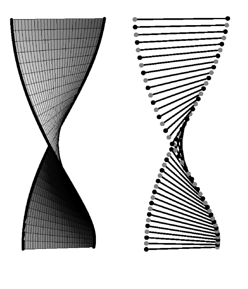
Figure 1:

Figure 2:

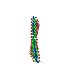
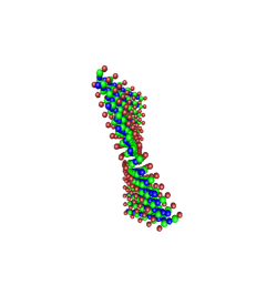
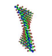
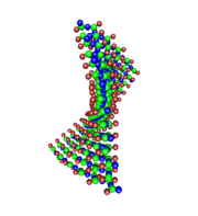
Figure 3:

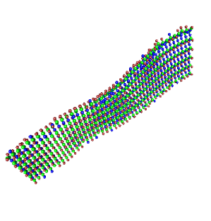
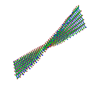
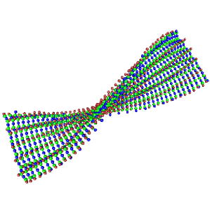
Figure 4:

Figure 5: