Incommensurate Mott Insulator in One-Dimensional Electron Systems close to Quarter Filling

Abstract

A possibility of a metal-insulator transition in molecular conductors has been studied for systems composed of donor molecules and fully ionized anions with an incommensurate ratio close to 2:1 based on a one-dimensional extended Hubbard model, where the donor carriers are slightly deviated from quarter filling and under an incommensurate periodic potential from the anions. By use of the renormalization group method, interplay between commensurability energy on the donor lattice and that from the anion potential has been studied and it has been found that an “incommensurate Mott insulator” can be generated. This theoretical finding will explain the metal-insulator transition observed in (MDT-TS)(AuI₂)_0.441.

Most of the conducting molecular crystals are realized by combining two kinds of molecules, $A$ and $B$, with commensurate composition ratios. Typical examples are the well-studied 2:1 compounds, i.e., $A_{2}B$, which show a variety of phases such as Mott insulator, charge order, superconductivity and so on. [1, 2] In the compounds, the molecule $B$ is usually fully ionized either as $-1$ or $+1$ to form a closed shell, and as a consequence the energy band formed by HOMO or LUMO of $A$ is quarter-filled as a whole in terms of holes or electrons, respectively.

Recently, molecular conductors with incommensurate (IC) composition ratios close to 2:1 have been synthesized based on new donor molecules. [3, 4, 5] (MDT-TSF)$X_{n}$ and (MDT-ST)$X_{n}$ ($X$ = I₃, AuI₂ or IBr₂, $n$ $\simeq$ 0.42 – 0.45) show metallic behavior and undergo superconducting transition at about $T_{c}$ = 4 K at ambient pressure. [3, 4] In contrast, in (MDT-TS)(AuI₂)_0.441 a metal-insulator (MI) crossover occurs where the temperature dependence of resistivity displays a minimum at $T_{\rho}$ = 85 K. [5] In addition, an antiferromagnetic transition takes place at $T_{\rm N}$ = 50 K. When pressure is applied to this compound, $T_{\rho}$ decreases and the superconducting phase appears above $P_{c}$ = 10.5 kbar ($T_{c}$ = 3 K). All these compounds are isostructural with alternating donor and anion layers. Since the anions are fully ionized as $X^{-}$ as in the 2:1 compounds, [3] the electronic properties can be attributed to the donors with the IC band-filling slightly larger than 3/4 for the HOMO bands. The extended H$\ddot{\rm u}$ckel scheme predicts two-dimensional (2D) Fermi surfaces which are similar to each other. [4, 5] It should be noticed that the anions in these compounds are not randomly distributed in the layers, but are found by the X-ray scattering experiments to form regular IC lattices with a different periodicity from the donors. [3, 4]

The metallic state observed in these compounds is naturally expected from the IC band-filling since the system would avoid insulating states due to strong correlation such as Mott insulator or charge order. On the other hand, it is difficult to understand the strong-coupling nature of the insulating ground state in (MDT-TS)(AuI₂)_0.441, deduced from $T_{\rho}\neq T_{\rm N}$, which is to be explored in this Letter; if it is the weak-coupling spin-density-wave state due to the nesting of the Fermi surface, $T_{\rho}=T_{\rm N}$ would be expected. [1]

We consider a one-dimensional (1D) model in order to capture the essence of the MI transition in a more controlled way than considering a 2D model relevant to experiments. Our 1D model consists of $N_{L}$ donor molecules coupled with $N$ anions both forming regular lattices, as shown in the inset of Fig. 1. The donors are modeled by the 1D extended Hubbard model, known to be relevant for typical 2:1 systems, [6, 7] and the small potential from the anions is added, which is crucial for the insulating state to appear. The Hamiltonian is written as follows,

$${\cal H} = -t\sum_{j,s}(c_{j+1,s}^{\dagger}c_{j,s}+h.c.)+\frac{U}{2}\sum_{j,s}n_{j,s}n_{j,-s}$$ (1)

$$+ V\sum_{j}n_{j}n_{j+1}+\sum_{j}v_{j}n_{j},$$

where $t$, $U$ and $V$ are respectively the transfer energy between the nearest-neighbor donor sites, the on-site repulsive interaction and the nearest-neighbor repulsion; the creation operator at the $j$-th site with spin $s$=$\pm$ is denoted as $c^{\dagger}_{j,s}$, $n_{j,s}=c^{\dagger}_{j,s}c_{j,s}$ and $n_{j}=\sum_{s}n_{j,s}$. Since the fully ionized anions form a regular lattice, the anion potential at the $j$-th site, $v_{j}$, can be expressed as $v_{j}=N_{L}^{-1}\sum_{m=-\infty}^{\infty}v(mQ){\rm e}^{{\rm i}mQja}$ where $Q=4k_{F}$, $k_{F}=\pi n/(2a)$ is the Fermi wavenumber, $n=N/N_{L}$ is the carrier density (we take the hole picture in the following) in the donor chain and $a$ is the spacing between donor sites. In the following, we consider only the relevant $\pm Q$ component of the potential, $v(\pm Q)\equiv v_{0}{\rm e}^{\pm{\rm i}\chi}$. This can lead to a gap, $2v_{0}$, at $\pm 2k_{\rm F}$ in the non-interacting band, which we assume to be small compared to the band width. Then the system becomes effectively half-filled in reference to the IC lattices as is seen in Fig.1.

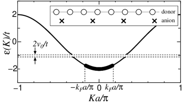
Figure 1: Energy dispersion in the presence of the anion potential $v_{0}=0.1t$ where the occupied one-particle states are expressed by the thick curve. The figure is written in the case of $n=0.33$ to clarify the characteristics of the present model. Inset: a schematic representation of our model.

We derive an effective Hamiltonian for low energy scale in terms of phase variables following the just quarter-filling case.[7] To the lowest order of the normalized anion potential $\delta\equiv v_{0}/\left\{\epsilon(3k_{F})-\epsilon(k_{F})\right\}$ with $\epsilon(K)=-2t\cos Ka$, the phase Hamiltonian is obtained as ${\cal H}_{\rm eff}={\cal H}_{\rho}+{\cal H}_{\sigma}+{\cal H}_{\rm\rho\sigma}$. Here ${\cal H}_{\rho}$, ${\cal H}_{\sigma}$ and ${\cal H}_{\rho\sigma}$ are respectively the charge part, the spin part and the term mixing both degrees of freedom. The spin part, ${\cal H}_{\sigma}$ has the same form as that of the 1D Hubbard model, so the spin excitation becomes gapless. [8] The term ${\cal H}_{\rho\sigma}$ is expressed by the product of the non-linear terms seen in ${\cal H}_{\rho}$ and ${\cal H}_{\sigma}$, and then has a larger scaling dimension. Hence we can neglect it [9]. Therefore the properties of the charge degree of freedom are determined by ${\cal H}_{\rho}$, expressed as

$${\cal H}_{\rho} = \frac{v_{\rho}}{4\pi}\int dx\left\{\frac{1}{K_{\rho}}(\partial_{x}\theta_{\rho})^{2}+K_{\rho}(\partial_{x}\phi_{\rho})^{2}\right\}$$ (2)

$$+ \frac{g_{3\bot}}{(\pi\alpha)^{2}}\int dx\cos(2\theta_{\rho}+3\chi)$$

$$+ \frac{g^{\prime\prime}_{3\bot}}{(\pi\alpha)^{2}}\int dx\cos(2\theta_{\rho}+5\chi-q_{0}x)$$

$$+ \frac{g_{1/4}}{2(\pi\alpha)^{2}}\int dx\cos(4\theta_{\rho}+8\chi-q_{0}x).$$

Here $q_{0}=2\pi/a-8k_{\rm F}=2\pi(1-2n)/a$ is the misfit parameter, $v=2ta\sin k_{\rm F}a$, $v_{\rho}=v\sqrt{B_{\rho}A_{\rho}}$ and $K_{\rho}=\sqrt{B_{\rho}/A_{\rho}}$ with $A_{\rho}=1+(g_{4||}+g_{4\bot}+g_{2||}+g_{2\bot}-g_{1||})/(\pi v)$ and $B_{\rho}=1+(g_{4||}+g_{4\bot}-g_{2||}-g_{2\bot}+g_{1||})/(\pi v)$. $\alpha^{-1}$ is the ultra-violet cut-off ($\alpha\sim a$). The interaction parameters are written as

$$g_{1||} = Va\cos 2k_{F}a$$ (3)

$$- 4D_{1}\left(Va\cos 2k_{F}a\right)\left(Va\cos 4k_{F}a\right),$$

$$g_{2\bot} = \frac{Ua}{2}+Va-2D_{1}$$

$$\times\left\{\left(\frac{Ua}{2}+Va\cos 2k_{F}a\right)^{2}+\left(\frac{Ua}{2}+Va\cos 4k_{F}a\right)^{2}\right\},$$

$$g_{2||} = Va$$ (5)

$$- 2D_{1}\left\{\left(Va\cos 2k_{F}a\right)^{2}+\left(Va\cos 4k_{F}a\right)^{2}\right\},$$

$$g_{3\bot} = -4\delta(\frac{Ua}{2}+Va\cos 2k_{F}a)$$ (6)

$$+ 4\delta D_{2}(\frac{Ua}{2}+Va\cos 4k_{F}a)$$

$$\times\left(Ua+Va\cos 2k_{F}a+Va\cos 6k_{F}a\right),$$

$$g^{\prime\prime}_{3\bot} = -4\delta D_{2}(\frac{Ua}{2}+Va\cos 4k_{F}a)$$ (7)

$$\times(Ua+2Va\cos 2k_{F}a),$$

$$g_{4\bot} = \frac{Ua}{2}+Va-2D_{2}\left(\frac{Ua}{2}+Va\cos 4k_{F}a\right)^{2},$$ (8)

$$g_{4||} = Va-2D_{2}\left(Va\cos 4k_{F}a\right)^{2},$$ (9)

$$g_{1/4} = \frac{X}{2(\pi\alpha)^{2}(\epsilon(3k_{F})-\epsilon(k_{F}))^{2}},$$ (10)

$$X = 2\Big{\{}(2Va\cos 2k_{F}a)^{2}(Ua+2Va\cos 4k_{F}a)$$ (11)

$$+ (Ua+2Va\cos 2k_{F}a)^{2}(Ua+4Va\cos 4k_{F}a)$$

$$+ (2Va\cos 2k_{F}a)(Ua+2Va\cos 2k_{F}a)$$

$$\times(Ua+Va\cos 2k_{F}a+Va\cos 6k_{F}a)\Big{\}}$$

$$+ (Ua+2Va\cos 2k_{F}a)^{2}$$

$$\times(Va\cos 2k_{F}a+Va\cos 6k_{F}a),$$

with

$$D_{1} = \frac{1}{4\pi v(3k_{F})}$$ (12)

$$\times\ln\frac{\epsilon(3k_{F})-\epsilon(k_{F})+v(3k_{F})k_{F}}{\epsilon(3k_{F})-\epsilon(k_{F})-v(3k_{F})k_{F}},$$

$$D_{2} = \frac{1}{4\pi}\frac{2k_{F}}{\epsilon(3k_{F})-\epsilon(k_{F})},$$ (13)

where $v(3k_{F})=2ta\sin 3k_{F}a$.

In eq.(2), there are three non-linear terms. First, the half-filling Umklapp term, $g_{3\bot}$, is generated by the anion potential $\delta$ because the band is effectively half-filled as seen in Fig.1. This can lead to a Mott insulator, as we will later show explicitly. We call the state as IC Mott insulator since it has a periodicity not matching with the donors but with the anions. However, it is not trivial whether this IC Mott insulator can be realized, and if so, in which condition it is stabilized, in contrast to the half-filled Hubbard model where infinitesimal on-site repulsion stabilizes the Mott insulator. [8] This is because of the presence of the other two non-linear terms in eq.(2), the “quarter-filling” Umklapp term, $g_{1/4}$, with the misfit which is present even without the anions owing to the proximity to a quarter filling on one hand, and the $g^{\prime\prime}_{3\bot}$ term, the combination of both commensurabilities of the donors and the anions on the other hand.

In the present calculation, it is crucial to fix the carrier number at the value determined by the anion density. However, it is to be noted that if one evaluates the quantity based on eq.(2), it results in a deviation of the carrier number from the value in the non-interacting case, $\Delta N_{e}=(1/L\pi)\int{\rm d}x\langle\partial_{x}\theta_{\rho}\rangle$, as

$$\Delta N_{e}/L = \frac{2K_{\rho}G_{3\bot}^{{}^{\prime\prime}2}}{\pi\alpha}\int_{\alpha}^{\infty}\frac{{\rm d}r}{\alpha}\left(\frac{r}{\alpha}\right)^{2-4K_{\rho}}J_{1}(q_{0}r)$$ (14)

$$+\frac{4K_{\rho}G_{1/4}^{2}}{\pi\alpha}\int_{\alpha}^{\infty}\frac{{\rm d}r}{\alpha}\left(\frac{r}{\alpha}\right)^{2-16K_{\rho}}J_{1}(q_{0}r)\neq 0,$$

where $G^{\prime\prime}_{3\bot}=g^{\prime\prime}_{3\bot}/(\pi v_{\rho})$, $G_{1/4}=g_{1/4}/(2\pi v_{\rho})$, and $J_{n}(x)$ is the the Bessel function of the first kind. The origin of the deviation is the existence of the misfit parameter. [10] Therefore, we must add the term, $-(\mu/\pi)\int{\rm d}x\partial_{x}\theta_{\rho}$ and keep $\Delta N_{e}$ to zero. To the lowest order of $G^{\prime\prime}_{3\bot}$ and $G_{1/4}$, the chemical potential $\mu$ is given as,

$$q_{\mu}\alpha = -4K_{\rho}G_{3\bot}^{\prime\prime 2}\int_{\alpha}^{\infty}\frac{{\rm d}r}{\alpha}(\frac{r}{\alpha})^{2-4K_{\rho}}J_{1}(q_{0}\alpha)$$ (15)

$$-8K_{\rho}G_{1/4}^{2}\int_{\alpha}^{\infty}\frac{{\rm d}r}{\alpha}(\frac{r}{\alpha})^{2-16K_{\rho}}J_{1}(q_{0}\alpha),$$

where $q_{\mu}=4K_{\rho}\mu/v_{\rho}$.

To determine the low energy behavior of this effective Hamiltonian, we derive the renormalization group (RG) equations by rewriting the action $S_{\rho}$ corresponding to the Hamiltonian, ${\cal H}_{\rho}-(\mu/\pi)\int{\rm d}x\partial_{x}\theta_{\rho}$, as

$$S_{\rho} = \frac{1}{4\pi K_{\rho}}\int{\rm d}^{2}\vec{r}\left\{(\partial_{x}\tilde{\theta}_{\rho})^{2}+(\partial_{y}\tilde{\theta}_{\rho})^{2}\right\}$$ (16)

$$+ \frac{G_{3\bot}}{\pi\alpha^{2}}\int{\rm d}^{2}\vec{r}\cos\left\{2\tilde{\theta}_{\rho}+3\chi-(q_{1/4}-q_{3}^{\prime\prime})x\right\}$$

$$+ \frac{G^{\prime\prime}_{3\bot}}{\pi\alpha^{2}}\int{\rm d}^{2}\vec{r}\cos\left\{2\tilde{\theta}_{\rho}+5\chi-q_{3}^{\prime\prime}x\right\}$$

$$+ \frac{G_{1/4}}{\pi\alpha^{2}}\int{\rm d}^{2}\vec{r}\cos\left\{4\tilde{\theta}_{\rho}+8\chi-q_{1/4}x\right\},$$

where $\tilde{\theta}_{\rho}=\theta_{\rho}-q_{\mu}x/2$, $G_{3\bot}=g_{3\bot}/(\pi v_{\rho})$, $q_{1/4}=q_{0}-2q_{\mu}$ and $q^{\prime\prime}_{3}=q_{0}-q_{\mu}$. The condition, $\Delta N_{e}=0$, leads to the following self-consistent equation,

$$q_{\mu}\alpha = -4K_{\rho}G_{3\bot}^{2}\int_{\alpha}^{\infty}\frac{{\rm d}r}{\alpha}(\frac{r}{\alpha})^{2-4K_{\rho}}\tilde{J}_{1}((q_{1/4}-q_{3}^{\prime\prime})\alpha)$$ (17)

$$-4K_{\rho}G_{3\bot}^{\prime\prime 2}\int_{\alpha}^{\infty}\frac{{\rm d}r}{\alpha}(\frac{r}{\alpha})^{2-4K_{\rho}}\tilde{J}_{1}(q_{3}^{\prime\prime}\alpha)$$

$$-8K_{\rho}G_{1/4}^{2}\int_{\alpha}^{\infty}\frac{{\rm d}r}{\alpha}(\frac{r}{\alpha})^{2-16K_{\rho}}\tilde{J}_{1}(q_{1/4}\alpha),$$

where $\tilde{J}_{1}(x)={\rm sgn}(x)J_{1}(|x|)$. Eqs.(16) and (17) lead to the following RG equations,

$${d\over{dl}}\,K_{\rho} = -8K_{\rho}^{2}G_{1/4}^{2}J_{0}(|q_{1/4}\alpha|)$$ (18)

$$-2K_{\rho}^{2}G_{3\bot}^{2}J_{0}(|q_{1/4}\alpha-q_{3}^{\prime\prime}\alpha|)$$

$$-2K_{\rho}^{2}G_{3\bot}^{\prime\prime 2}J_{0}(|q_{3}^{\prime\prime}\alpha|),$$

$${d\over{dl}}\,q_{1/4}\alpha = q_{1/4}\alpha-16K_{\rho}G_{1/4}^{2}\tilde{J}_{1}(q_{1/4}\alpha)$$ (19)

$$-8K_{\rho}G_{3\bot}^{2}\tilde{J}_{1}(q_{1/4}\alpha-q_{3}^{\prime\prime}\alpha)$$

$$-8K_{\rho}G_{3\bot}^{\prime\prime 2}\tilde{J}_{1}(q_{3}^{\prime\prime}\alpha),$$

$${d\over{dl}}\,q_{3}^{\prime\prime}\alpha = q_{3}^{\prime\prime}\alpha-8K_{\rho}G_{1/4}^{2}\tilde{J}_{1}(q_{1/4}\alpha)$$ (20)

$$-4K_{\rho}G_{3\bot}^{2}\tilde{J}_{1}(q_{1/4}\alpha-q_{3}^{\prime\prime}\alpha)$$

$$-4K_{\rho}G_{3\bot}^{\prime\prime 2}\tilde{J}_{1}(q_{3}^{\prime\prime}\alpha),$$

$${d\over{dl}}\,G_{3\bot} = (2-2K_{\rho})G_{3\bot}$$ (21)

$$-G_{3\bot}^{\prime\prime}G_{1/4}J_{0}(|(q_{3}^{\prime\prime}\alpha+q_{1/4}\alpha)/2|),$$

$${d\over{dl}}\,G_{3\bot}^{\prime\prime} = (2-2K_{\rho})G_{3\bot}^{\prime\prime}$$ (22)

$$-G_{3\bot}G_{1/4}J_{0}(|q_{1/4}\alpha-q_{3}^{\prime\prime}\alpha/2|),$$

$${d\over{dl}}\,G_{1/4} = (2-8K_{\rho})G_{1/4}$$ (23)

$$-G_{3\bot}G_{3\bot}^{\prime\prime}J_{0}(|q_{3}^{\prime\prime}\alpha-q_{1/4}\alpha/2|),$$

$${d\over{dl}}\,q_{\mu}\alpha = q_{\mu}\alpha+4K_{\rho}G_{3\bot}^{2}\tilde{J}_{1}((q_{1/4}-q_{3}^{\prime\prime})\alpha)$$ (24)

$$+4K_{\rho}G_{3\bot}^{\prime\prime 2}\tilde{J}_{1}(q^{\prime\prime}_{3}\alpha)$$

$$+8K_{\rho}G_{1/4}^{2}\tilde{J}_{1}(q_{1/4}\alpha).$$

Eqs.(18)-(23) are obtained for the condition of the action, eq.(16), being invariant under RG transformation, whereas eq.(24) is obtained from the condition of the chemical potential, eq.(17). From eqs.(19), (20) and (24), it is shown that the quantity $q_{0}$, whose dimension is $({\rm length})^{-1}$, is scaled as $q_{0}(l)=q_{0}{\rm e}^{l}$. This shows the fact that the carrier number is indeed conserved without any effects from the interaction.

Typical flows of the RG equations are shown in Fig.2 for $U/t=3.0$ and $V/t=0.0$ where the carrier number is fixed as $n=0.441$ taken from the actual material (MDT-TS)(AuI₂)_0.441.

Figure 2: The solutions of the RG equations, $K_{\rho}$ and $(q_{1/4}-q_{3}^{\prime\prime})\alpha$ ( the misfit parameter of the $G_{3\bot}$-term ) for $U/t=3.0$, $V/t=0.0$ and $n=0.441$. The cases of $\delta=0.001$ and $0.005$ are denoted by the solid and dotted curves, respectively.

In the case of $\delta=0.005$, $K_{\rho}$ tends to zero implying that the ground state is an insulator, due to the commensurability in the half-filling, $G_{3\bot}$. This can be seen in the RG equations since the misfit parameter in the $G_{3\bot}$-term, $(q_{1/4}-q_{3}^{\prime\prime})\alpha=-q_{\mu}\alpha$ vanishes (see Fig.2) and then $G_{3\bot}$ affects the renormalization of $K_{\rho}$ through eq.(18) while those in the $G_{1/4}$- and $G_{3\bot}^{\prime\prime}$-terms, $q_{1/4}\alpha$ and $q_{3}^{\prime\prime}\alpha$, tend to $\infty$ and then these effects become negligible due to the oscillating behavior of the Bessel function. Hence the origin of this insulating state is nothing but the commensurate potential of the effective half-filling generated by the anion potential. Namely, the insulating state is indeed the IC Mott insulator.

On the other hand, in the case of smaller potential due to the anions, $\delta=0.001$, a metallic state with finite value of $K_{\rho}$ is realized. Here in eq.(18) the effects of the $G_{3\bot}$-, $G^{\prime\prime}_{3\bot}$- and $G_{1/4}$-terms on $K_{\rho}$ disappear at the low energy since all the misfit parameters are divergent. This metallic state is not realized if we set $G_{1/4}$ to zero. Therefore we can state that the origin of the MI transition is the interplay between the different kinds of commensurabilities.

Next, we show ground state phase diagrams as a function of the model parameters. First, the phase diagram on the plane of $U/t$ and $\delta$ in the case of $V/t=0$ is shown in Fig.3.

Figure 3: The phase diagram on the plane of $\delta$ and $U/t$ in the case of $V/t=0$ and $n=0.441$.

Figure 4: The phase diagram on the plane of $\delta$ and $V/t$ in the case of $U/t=3.0$ and $n=0.441$.

Since the quantity $\delta$ is proportional to $v_{0}/t$, the transition from the metallic state to the IC Mott insulator occurs when the potential from the anions increases and/or the band width decreases. When $U$ $\to$ $\infty$, the present system can be mapped onto a non-interacting spinless Fermion system with the Fermi wavenumber doubled, as $2k_{\rm F}$.[11] In this case the insulating state is realized by an infinitesimal $\delta$ because a gap opens at $\pm 2k_{\rm F}$ (see Fig.1), consistent with Fig.3.

The role of the $G_{1/4}$-term on the MI transition becomes clearer when $V$ is varied. It is because the coupling constant $G_{1/4}$ changes its sign when $V$ increases.[7] We show the phase diagram on the $V/t$ - $\delta$ plane in Fig. 4 for $U/t=3.0$. At $V=V_{c}=0.838t$ where $G_{1/4}=0$, the IC Mott insulating state is realized for infinitesimal $\delta$. For $V>V_{c}$, the absolute value of $G_{1/4}$ increases again and results in a finite metallic region. Therefore, a re-entrant transition, metal $\to$ IC Mott insulator $\to$ metal, occurs when $V$ increases. Note that there is no qualitative difference between the metallic states in the two distinct regions.

Finally let us discuss the relevance of our results to the experiments. The difference of the ground state in metallic MDT-TSF and MDT-ST compounds and that in the MDT-TS compound undergoing MI crossover can be naturally understood as follows. The extended H$\ddot{\rm u}$ckel scheme provides transfer integrals, i.e., the band width, of the MDT-TSF families larger than that of the MDT-TS compound [4, 5], which is consistent with our results that the decrease of the bandwidth lead to an MI transition, as seen in Fig.3. In our 1D model the spin degree of freedom is essentially that of the 1D Heisenberg model showing no magnetic order. However, in the IC Mott insulating state in the actual 2D material we generally expect that antiferromagnetic order appears at low temperature due to the three dimensionality, as in fact observed. [5] In this case, the magnetic ordered moment should be large, compared to, e.g., that of the spin-density-wave state due to the nesting of the Fermi surface.

In conclusion, we investigated the electronic state of the one-dimensional extended Hubbard model close to quarter-filling under an incommensurate anion potential. We found that a transition between the metallic state and an incommensurate Mott insulator can occur, whose origin is the interplay between the commensurability energy generated by the anion potential and that in the donor lattice. To the authors’ best knowledge this is the first theoretical study of a “Mott transition” generated by such interplay between different commensurabilities. It would be interesting to investigate the critical properties of this transition in the actual compounds and compare with the “usual” Mott transition seen in the typical 2D $A_{2}B$ molecular conductors, $\kappa$-(BEDT-TTF)${}_{2}X$, which is recently attracting interests. [12]

The authors would like to thank T. Kawamoto for sending them his preprint prior to publication. They also acknowledge G. Baskaran, M. Ogata, K. Kanoda, and J. Kishine for valuable discussions and comments. This work was supported by Grant-in-Aid for Scientific Research on Priority Area of Molecular Conductors (No.15073213) and Grant-in-Aid for Scientific Research (C) (No. 14540302 and 15540343) from MEXT.

References

[1]
T. Ishiguro, K. Yamaji and G. Saito:
Organic Superconductors
(Springer-Verlag, Berlin, 1998) 2nd ed.
[2]For various recent reviews, Chem. Rev. 104 (2004) No.11.
[3]
K. Takimiya et al., : Angew. Chem. Int. Ed. 40 (2001) 1122;
Chem. Mat. 15 (2003) 1225; ibid. 3250.
[4]
T. Kawamoto et al., : Phys. Rev. B 65 (2002) 140508;
ibid.67 (2003) 020508(R);
Eur. Phys. J. B 36 (2003) 161; J. Phys. IV France 114 (2004) 517.
[5]
T. Kawamoto et al., : preprint.
[6]
H. Seo, C. Hotta and H. Fukuyama:
Chem. Rev. 104 (2004) 5005.
[7]
H. Yoshioka, M. Tsuchiizu and Y. Suzumura:
J. Phys. Soc. Jpn. 69 (2000) 651; ibid.70 (2001) 762.
[8]V. J. Emery: in Highly Conducting One-Dimensional
Solids, ed. J. Devresse, R. Evrard, and V. Van Doren
(Plenum, New York, 1979), p. 247.
[9]
The spin-charge coupled term plays an essential role when
the coefficients of the non-linear terms of both degree of freedom
vanish (see M. Tsuchiizu and A. Furusaki:
Phys. Rev. Lett. 88 (2002) 056402), which does not happen in the present case.
[10]
M. Mori, H. Fukuyama and M. Imada:
J. Phys. Soc. Jpn. 63 (1994) 1639.
[11]
A.A. Ovchinnikov:
Sov. Phys.-JETP 37 (1973) 176;
M. Ogata and H. Shiba:
Phys. Rev. B 41 (1990) 2326.
[12]S. Lefebvre et al., : Phys. Rev. Lett. 85 (2000) 5420;
F. Kagawa et al., : Phys. Rev. B 69 (2004) 064511.