Racing downhill: optimization and the random-field Ising model

Abstract

The push-relabel algorithm can be used to calculate rapidly the exact ground states for a given sample with a random-field Ising model (RFIM) Hamiltonian. Although the algorithm is guaranteed to terminate after a time polynomial in the number of spins, implementation details are important for practical performance. Empirical results for the timing in dimensions $d=1,2,\textrm{ and }3$ are used to determine the fastest among several implementations. Direct visualization of the auxiliary fields used by the algorithm provides insight into its operation and suggests how to optimize the algorithm. Recommendations are given for further study of the RFIM.

I Introduction

In systems with quenched disorder, changes in the random background take place over time scales that are much longer than the time scale for evolution of the primary degrees of freedom. In magnetic systems, the spin degrees of freedom interact in an effectively frozen random environment determined by substitutional disorder or vacancies. The random-field Ising model (RFIM), defined as ferromagnetically-coupled spins subject to a spatially varying magnetic field, is a prototypical model for magnets with quenched disorder that has been studied since the 1970s (for reviews, see, e.g., Young (1998)). In dimensions $d>2$, the RFIM has a transition between ferromagnetic (FM) and paramagnetic (PM) states; this transition can be found by varying either the temperature or the disorder, at sufficiently small values of the remaining control parameter. Fishman and Aharony Fishman and Aharony (1979) mapped the RFIM with a field of random sign and fixed magnitude with disordered bonds to an experimentally realizable system: the diluted antiferromagnet in a field (DAFF) Belanger (1998). At low temperatures, the glassy behavior of the DAFF seen in both experiment and theory leads to non-equilibrium effects such as history dependence and a broad range of relaxation times. These observations are qualitatively consistent with predictions by both Fisher and Villain of an exponential slowing down near the critical point and of a low temperature phase described by the zero-temperature critical point Villain (1984); Fisher (1986).

Exponential slowing down also affects optimization methods such as simulated annealing Kirkpatrick et al. (1983), that are modeled on the dynamics of the physical system. The large barriers to equilibration make it very time consuming to sample configuration space accurately at finite temperatures or to find the exact zero-temperature ground states using such methods. Finding the partition function for the RFIM at finite temperature is NP-hard J. C. Angles d’Auriac et al. (1985); Sorin Istrail (1999). However, the zero-temperature FM-PM transition is expected to be in the same universality class as the finite temperature transition. So it is fortunate that there are alternate methods for quickly finding the exact RFIM ground state. These methods are based on a mapping from the problem of finding the ground state of the RFIM to that of finding the maximum flow—or, equivalently, the minimum cut—in a capacitated graph Picard and Ratliff (1975); Barahona (1985); Ogielski (1986). Ogielski’s computations of the RFIM ground state properties Ogielski (1986) utilized the push-relabel (PR) algorithm for max-flow introduced by Goldberg and Tarjan Goldberg and Tarjan (1988). The PR algorithm is in practice the most efficient algorithm available for many classes of problems Cherkassky and Goldberg (1997a). Although its generic implementation has a polynomial time bound, its actual performance depends on the order in which operations are performed and which heuristics are used to maintain auxiliary fields for the algorithm. Even within this polynomial time bound, there is a power-law critical slowing down of the PR algorithm at the zero-temperature ($T=0$) transition Ogielski (1986); Middleton and Fisher (2002); Middleton (2002).

This paper presents results that are useful for minimizing CPU time in RFIM ground-state simulations. We begin with a brief review of the RFIM, including its definition and phases, in Sec. II. We then discuss the implementations for the PR algorithms that we study. The PR algorithm redistributes the random magnetic field among spins by pushing positive field “downhill” with respect to a potential field (the “height”) defined for each spin. This redistribution and coalescence of positive field and negative field “sinks” allows for the determination of same-spin domains. The data structures used to organize the pushes and the heuristics used for updating the potential field are described in Sec. III. The results for the timing using various heuristics, summarized in Sec. IV, should be useful for designing further extensive studies of the RFIM. Visualizing the auxiliary fields leads to a clearer explanation of the timing results and was important in guiding our work. In Sec. V, we use these visualizations to present a qualitative overview of the operations of the different implementations in the distinct phases of the RFIM. The primary results of the paper, namely the recommended choices for the PR algorithm, are summarized in Sec. VI.

II Random-field Ising model

The random-field Ising model has a non-trivial ground state due to the competition between the ferromagnetic interaction that tends to align neighboring spins and the influence of random fields, which tends to force spins to point in random directions. Taking the strength of the ferromagnetic interactions between neighboring spins to be $J$ and designating the local random fields by $h_{i}$, the energy of a spin configuration is Young (1998)

$$\mathcal{H}=-J\sum_{\langle ij\rangle}s_{i}s_{j}-\sum_{i}h_{i}s_{i},$$ (1)

where the spin $s_{i}$ at a given site $i$ on a $d$-dimensional lattice with $n=L^{d}$ sites can take on values $s_{i}=\pm 1$ and the sites $i$ and $j$ in the sum in the first term are nearest neighbors. We study the Gaussian RFIM, where the $h_{i}$ are independent variables chosen from a Gaussian distribution with mean $0$ and variance $\Delta^{2}J^{2}$, with periodic boundary conditions. The parameter $\Delta$ characterizes the strength of the disorder relative to the ferromagnetic interaction.

As the disorder dominates over thermal fluctuations at large length scales and low temperature in more than two dimensions, the ground states of this model are of interest. In dimensions $d>2$, there is a zero-temperature transition between two phases at the critical disorder $\Delta=\Delta_{c}$. When $\Delta<\Delta_{c}$, the ferromagnetic interaction between nearest neighbors dominates and the spins take on a mean value $m=n^{-1}\sum_{i}s_{i}$ with $\left|m\right|\neq 0$ in the limit $n\rightarrow\infty$. In the case $\Delta>\Delta_{c}$, randomness dominates and the ground state is “paramagnetic” $\left|m\right|=0$, as $n\rightarrow\infty$.

In dimensions $d=1\textrm{ and }2$, the ground state is in the paramagnetic phase at any $\Delta>0$ in the thermodynamic limit (i.e., $\Delta_{c}=0$). But the correlation length $\xi$, characterizing the range of spin-spin correlations or the size of uniform spin domains, diverges as $\Delta^{-2}$ when $d=1$ (see, e.g., Schröder et al. (2002)). For samples of size $L\ll\xi$, i.e., for $\Delta<\Delta_{x}\sim L^{-1/2}$, where $\Delta_{x}(L)$ is the sample-size-dependent crossover disorder, the ground state is essentially ferromagnetic. It has been argued that $\ln(\xi)$ scales as an inverse power of $\Delta$ when $d=2$ Binder (1983); Grinstein and k. Ma (1982); Seppälä and Alava (2001). This very rapidly growing correlation length gives rise to an apparent ferromagnetic phase in $d=2$ at even moderate $\Delta_{x}$ in finite samples Alava and Rieger (1998). When we take the limit $\Delta\rightarrow 0$ in $d=1$ and $d=2$, we will be taking $\Delta\ll\Delta_{x}$. Many of the results for the algorithm, such as which algorithm is fastest, hold independently of the existence of a true physical phase transition.

III Push-Relabel Algorithm: Data Structures and Heuristics

We now discuss the motivation for using the PR algorithm and outline its structure. In particular, we define the auxiliary fields and basic operations that operate on those fields to determine the ground state. Picard and Ratliff showed that any quadratic optimization problem, such as the RFIM, can be mapped onto a min-cut/max-flow problem Picard and Ratliff (1975). There are a number of algorithms for solving max-flow Cormen et al. (1990), though Cherkassky and Goldberg’s results show that the PR algorithm Goldberg and Tarjan (1988) is often the best algorithm for solving large problems on a variety of graphs Cherkassky and Goldberg (1997a). For detailed explanations of the mapping of the RFIM to a max-flow problem and the proofs of the correctness of the PR algorithm, see reviews of applications of combinatorial optimization to statistical physics Alava et al. (2001); Hartmann and Rieger (2002); Middleton (2004) and computer science texts Cormen et al. (1990). In this paper, we limit ourselves to a description of the algorithm, neglecting proofs of correctness, but including a “physical” description for the variant of the PR algorithm we have used.

Intuitively, the PR algorithm finds the domains of uniform spin in the ground state by rearranging (“pushing”) the magnetic field. If the bond between two spins is strong enough, the field on one spin can be removed from one spin and added to its neighbor, possibly influencing the direction of the neighboring spin. This rearrangement (and change in the bonds, as described below) is the push. Subsequent pushes can then affect distant spins. As a consequence of pushes, positive and negative fields originally located on separate spins cancel. The cancellation leads to domains of uniform sign for the excess fields. This domain growth by rearrangement of field is limited by the strength of the nearest-neighbor bonds, which “carry” the rearrangement. The push operation reduces or removes the interactions between neighboring spins. When the field has large variations compared to the bond strengths, the magnetic field cannot be pushed very far as bonds become saturated and block further rearrangement. Conversely, in the limit of weak fields, large domains form, as the bonds favor alignment of nearest neighbor spins: in the language of PR, the large capacity of the bonds relative to the strength of the fields allows for long-range rearrangements of the random field. In the limit of very weak fields, the field can be pushed anywhere (no bonds are saturated), so there is only one domain, whose orientation is simply a result of the sum of the random fields on all the spins. But when the field is very strong ($\Delta\gg 1$), the rearrangement of field is limited, and, in most cases, the domains have single spins and the orientation of a spins is in the same direction as its magnetic field.

The other basic operation is the relabel operation. This operation updates an auxiliary field, the height, defined for each spin. Following the more detailed constraints described in Sec. III.1, this height guides the pushes. Most simply put, pushes are always in the downhill direction. When a push is not possible from a given site, the relabel operation increases the magnitude of the height of that site. This relabelling will either allow a push to be executed or will identify the spin as having a particular sign in the ground state.

The basic operations can be carried out using a variety of ordering methods. The choice of method affects the running time of the algorithm. A specific algorithm is defined by two sets of choices, which are defined and described in detail in the following subsections:

1. the dynamically-determined order local operations (pushes and relabels), which is organized by a choice of data structure, and

2. heuristic manipulations of the auxiliary fields, namely, global updates and gap relabeling.

We implemented the PR algorithm in Java and C++. The Java implementation can visualize the evolution of the auxiliary fields used by PR. The C++ code relied on the original C code Goldberg developed by Cherkassky and Goldberg Cherkassky and Goldberg (1997a). The codes can be downloaded from our web site Hambrick (2003).

III.1 Auxiliary fields and push-relabel operations

The PR algorithm uses three auxiliary fields to guide the rearrangement of the magnetic field and to enforce the constraints given by the bond strengths. One field is the residual bond strength (more commonly referred to as the residual capacity in the literature Cormen et al. (1990)). This residual interaction between sites is denoted $r_{ij}$. Initially, $r_{ij}=r_{ji}=J$ for all nearest neighbor pairs $(i,j)$, but in general $r_{ij}$ need not equal $r_{ji}$ during the execution of the algorithm. This residual bond strength defines the paths along which excess magnetic field can be pushed. A site $j$ is said to be reachable from a site $i$ if there is a directed path from $i$ to $j$ with $r_{kl}>0$ for all bonds $(k,l)$ along that path.

For each site $i$, an excess field $e_{i}$ and a height field $u_{i}$ (which is often called “distance” or “rank”) are also defined. At the beginning of the algorithm, the excess, which can be positive or negative, is set equal to the random field strength, $e_{i}=h_{i}$, and the height field $u_{i}$ is set equal to the distance to the nearest reachable site with negative excess. Sites from which no site with negative excess can be reached have $u_{i}=\infty$. Sites with negative excess have $u_{i}=0$.

The PR algorithm maintains the height field $u_{i}$ in a fashion designed to move the positive excess “downhill” (to smaller heights), i.e., towards sites with negative excess, where possible. If it becomes impossible to rearrange excess towards a site with negative excess, the site is given a height label $u_{i}=\infty$ (in practice, $\infty$ is represented by $n$, the number of spins). A site $j$ is said to be accessible from $i$ if the residual bond strength $r_{ij}>0$ and $u_{i}=u_{j}+1$. Any site with positive excess and height $u_{i}<\infty$ is active. (In the double queue method mentioned in Sec. III.2, negative excess sites can also be active.)

The push operation moves excess from an active site $i$ to an accessible neighbor $j$. Letting $\delta=\min(r_{ij},e_{i})$, the excesses are updated by $e_{i}\rightarrow e_{i}-\delta$, $e_{j}\rightarrow e_{j}+\delta$, while the residual bond strengths are updated according to $r_{ij}\rightarrow r_{ij}-\delta$ and $r_{ji}\rightarrow r_{ji}+\delta$. If an active site has no accessible neighbor, so that no pushes are possible, it is relabeled: the height $u_{i}$ is set to one greater than the height of the lowest neighbor $j$ (i.e., minimal $u_{j}$ over neighbors $j$) for which $r_{ij}>0$. If no such neighbor exists, the height of $i$ may immediately be raised to $u_{i}=\infty$. We call the combination of all possible push operations from a single spin possibly followed by a relabel a PR step.

The PR algorithm terminates when no active sites remain. The total number of PR steps needed to complete the algorithm is denoted by $N_{\mathrm{PR}}$. The assignment of spin orientations in the ground state is found by executing a global update (Sec. III.3) to finalize which sites have $u_{i}=\infty$. Sites with $u_{i}=\infty$ are assigned $s_{i}=1$, while the remaining spins have $s_{i}=-1$.

III.2 Data structures

We implemented the PR algorithm using four different data structures: a first-in-first-out queue (FIFO), a highest height priority queue implemented as a heap (HPQ), a lowest height priority queue (LPQ) also implemented as a heap, and a double FIFO queue (DFIFO) that treats positive and negative excess symmetrically. (We also tried a stack or last-in first-out (LIFO) structure, but rejected it due to vastly longer running times at large $\Delta$.)

The FIFO structure is a list of active sites in the lattice. The site at the front of the list, $i$, is removed. Excess is pushed away from $i$ if possible. If any inactive neighbors $j$ of $i$ are made active through a push operation, they are added to the end of the list. If there are no accessible neighbors, $i$ is relabeled. If $i$ is still active after this PR step, it is also appended to the end of the list.

The HPQ structure Cherkassky and Goldberg (1997b) is more complex than FIFO. Like the FIFO structure it contains a list of all active sites. The list is not organized by the temporal order in which sites have been treated, as would be the case in a FIFO queue, but by the height of the sites. The first site in the HPQ is always a site with maximal height. When we remove a site from the front of the queue, the site with the highest height that is still in the queue moves to the front. If we add a site with a larger height than any of the sites already in the queue, the new site moves to the front of the queue. If after a PR step a site is still active, it is re-added to the queue. Since a PR step relabels an active site by increasing its height by at least one before adding it back to the queue, such a site is still of maximal height and is added at the front. Thus the same site might be acted upon by the algorithm many times in a row. In practice, the HPQ is simply implemented by sorting the sites into bins given by their height values.

The LPQ structure A. V. Goldberg and R. Kennedy (1997) is exactly the same as the HPQ structure, except that the list is reversed, so that sites $i$ with lowest height $u_{i}$ are subject to PR operations.

FIFO, HPQ, and LPQ enforce an asymmetry between positive and negative excess. Why should one sign (positive excess) be pushed around while the other (negative excess) remains static (except by rearrangement of positive excess onto a negative excess of lesser magnitude)? Certainly, the physical problem is unaltered by the replacement $h_{i}\rightarrow-h_{i}$. Our fourth implementation treats positive and negative excesses on an equal footing. Negative excess then moves from lower heights (here, $u_{i}<0$ is a possible height label) to higher heights. We implemented this as two FIFO queues (DFIFO), one for positive and one for negative excess sites. Both queues are updated simultaneously. As noted in the next section, we also used two height fields, one for each sign of excess, when implementing DFIFO.

III.3 Heuristics

If these queues are adapted as described so far, the algorithm, though polynomial in $n$, is too slow to be practical for studying larger systems. Heuristics can be used to manipulate the height field to guide the push-relabel operations. Good heuristics are crucial to the practicality of the algorithm.

All our implementations use the “global update” heuristic for initialization of the $u_{i}$. A global update Cherkassky and Goldberg (1997a) is used for two purposes. It creates gradients in the height field from the sites with positive excess to the nearest site with negative excess, allowing the excess fields to move efficiently towards annihilation. It addition, it identifies regions that are disconnected from the rest of the spins and do not contain any negative excess; such regions are labeled as spin-up regions and are removed from further consideration. Without this identification it would take of the order of $nr$ operations to mark a region of $r$ spins as up. The global update is implemented as a breadth first search starting from the set of negative excess sites and takes of the order of $n$ operations on a hypercubic lattice. During this search, the height of each vertex is set to the distance to the nearest reachable site with negative excess (sink). One important result of global updates is that local minima of the height field with positive height, often residuals of former negative excess sites, are eliminated at sites with nonnegative excess. Following common practice, we choose the interval between global updates to be fixed, with a global update executed after every $\Gamma$ push-relabel (PR) steps.

The global update needs to be modified for the double queue (DFIFO) approach. In parallel with the height field for positive excess, based on a search from nodes with negative excess, it is natural to construct the height field for negative excess sites using positive excess sites as “sinks”. This creates an ambiguity for sites with zero excess. Should their height be determined in relation to the positive or negative excess sites? We did not directly resolve this ambiguity, but instead used a scheme with separate height fields for the positive and negative excesses, with separate relabeling and global updates.

In addition, when using the HPQ data structure, we use gap relabeling Cherkassky and Goldberg (1997a). If there is a height $u_{g}$, such that no site has height $u=u_{g}$, but there are active sites with $u>u_{g}$, i.e., there is a gap in the set of heights, all sites with $u>u_{g}$ are assigned the maximum height. This reduces the need for global updates as active sites with $u>u_{g}$ are disconnected from the sinks. When using HPQ, regions with larger height tend to have their height raised uniformly, leading to the possibility of creating a gap quickly. As the gap is a global tally, it is not efficient at detecting regions that have separated themselves from their surroundings locally, so gap relabeling is less useful in, e.g., FIFO, where updates are carried out without respect to height. To facilitate gap relabeling, the HPQ algorithm uses an array that contains the number of sites (whether active or not) at each possible height. A gap is created when the occupation number at a non-maximal height is reduced to zero.

IV Comparison of Implementations

To find the best available combination of data structure and heuristics for solving the Gaussian RFIM, we measured the running time of the algorithm for a variety of combinations. We measure the running time for the algorithm to find the ground state using both CPU time $t$ in seconds and the total number of PR steps $N_{\mathrm{PR}}$. PR steps are the core operations of the algorithm and give us a machine independent measure of the improvement due to the heuristics. However, PR steps don’t account for the time needed for the internal bookkeeping of the data structure, nor do they reflect the time needed for the heuristics, such as the global update. The CPU time $t$ is therefore another useful measure of the performance and ultimately what we want to minimize. For the timing measurement we used SUN’s Java Virtual Machine 1.4.2 on Dual 1GHz PIII machines with 512MB of RAM running Linux.

Here we summarize the results of our timing runs. We first describe our results for two-dimensional lattices. In this case there is no phase transition for the RFIM ground states at finite $\Delta$. However, as the correlation length $\xi$ diverges very rapidly as $\Delta$ decreases, there is a crossover disorder value $\Delta_{x}(L)$ at which $\xi$ exceeds the linear system size $L$. For $\Delta<\Delta_{x}(L)$, the 2D system is effectively ferromagnetic. The dependence of $\Delta_{x}$ on $L$ is very slow Binder (1983); Grinstein and k. Ma (1982); Seppälä and Alava (2001). In our simulations, we find $\Delta_{x}(8)\approx 1.7$ and $\Delta_{x}(4096)\approx 0.55$. In three dimensions, there is a true transition at $\Delta=\Delta_{c}\approx 2.27$ Middleton and Fisher (2002).

In this section, we compare the timings for FIFO and HPQ structures and then present results for DFIFO. (Results for LPQ are included in the discussion of the results for $d=3$, near the end of this section.) When seeking to minimize the running time, there is a competition between frequent global updates (small $\Gamma$), which improve the efficiency of the PR steps and infrequent updates (large $\Gamma$), which save the cost of performing a global update. We first determine the global update interval that minimizes the CPU time over all choices of $\Delta.$ Generally, for all data structures, we find a minimum in $t$ for $\Gamma_{\min}\approx n$ (or at least that performance is not improved for other $\Gamma$). The FIFO and HPQ structures then give comparable results away from the crossover $\Delta\approx\Delta_{x}$, though FIFO is preferable at small $\Delta$ and HPQ is faster at large $\Delta$. DFIFO takes significantly more time than either HPQ or FIFO to find the ground state for $\Delta$ on the order of $\Delta_{x}$. We also find that the discreteness of global updates can lead to plateaus in the number of global updates $N_{G}$ as a function of $\Gamma$. The 3D results are generally consistent with our results for 2D lattices. We find that LPQ always performs at least as well as HPQ and is faster for $\Delta>\Delta_{c}$.

IV.1 Choosing the global update interval in two dimensions

We first examine the effect of varying the update interval $\Gamma$ for two dimensional samples. Global updates are only useful if they reduce the number of PR steps needed to find the solution. As we mentioned in Sec. III.3, global updates are expensive, taking of the order of $n$ operations, and should therefore not be performed too frequently. To find the optimal update interval $\Gamma_{\min}$, we varied $\Gamma$ for each data structure over several orders of magnitude for various values of the random field strength $\Delta$ and examined how both $N_{\mathrm{PR}}$, the number of push-relabel cycles used to find the ground state, and the running time $t$ varied.

IV.1.1 Global update interval for FIFO

Immediately after a global update, push operations are guaranteed to move excess towards the nearest sinks. After a global update, however, some sinks are soon annihilated by excess pushed into them. If a sink at site $s$ is annihilated, the height field around $s$ no longer indicates the shortest distance to a sink; the height field still slopes towards $s$ although there is no longer a sink. The extent of this “misleading” height field depends on the density of sinks and is limited by the distance between sinks. When $\Gamma$ is small, global updates are frequent enough that the height field generally leads positive excess towards a sink. As long as this is the case, increasing the frequency of global updates does little to reduce $N_{\mathrm{PR}}$. Therefore, for small $\Gamma$, we expect $N_{\mathrm{PR}}$ to be almost independent of $\Gamma$ for FIFO.

Fig. 1 displays algorithm costs $N_{\mathrm{PR}}$ and $t$ for the case $\Delta=2.2$, which exceeds $\Delta_{x}$. The expectation that $N_{\mathrm{PR}}$ is independent of $\Gamma$ at small $\Gamma$ is confirmed by the plot of the mean of $N_{\mathrm{PR}}$ as a function of $\Gamma$ displayed in Fig. 1(a). As we increase $\Gamma$, a larger and larger fraction of the height field becomes incorrect between global updates: more minima of the height field no longer contain sinks. The plot shows that $N_{\mathrm{PR}}$ starts to increase significantly above $\Gamma\approx 0.1n$. To minimize the running time $t$, we need to balance the cost of additional global updates with the reduction in $N_{\mathrm{PR}}$. A global update takes of the order of $n$ operations and, in fact, Fig. 1(b) shows a minimum in $t$ vs. $\Gamma$ at $\Gamma_{{\rm min}}\approx n$. To verify our assumption that $\Gamma_{{\rm min}}\approx n$, we rescaled the curves in both Fig. 1(a) and (b) by dividing $\Gamma$, $N_{\mathrm{PR}}$, and $t$ by $n$. The collapse of the data verifies the minimum in $t$ vs. $\Gamma$ at $\Gamma_{{\rm min}}\approx n$ and shows that the running time of the algorithm scales nearly linearly with $n$ in 2D (Fig. 2), at fixed $\Delta$.

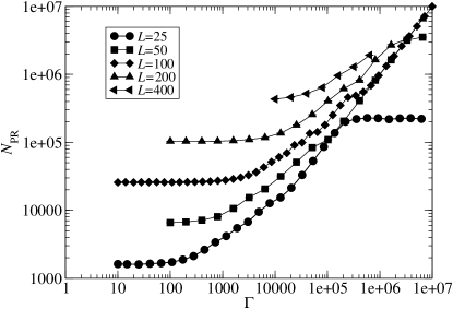
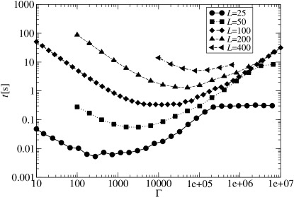
Figure 1: Mean running time for finding the ground state of a 2D RFIM system vs. $\Gamma$ using FIFO and $\Delta=2.2$, where the correlation length is much smaller than the sample sizes used, $\xi\ll L$. For clarity in this figure and other figures in this section, statistical error bars are not shown, but are consistent with the apparent deviations from smooth curves. The figure shows (a) the number of PR steps $N_{\mathrm{PR}}$ used to find the ground state and (b) CPU time $t[\textrm{s}]$ as a function of the global update interval $\Gamma$ for $L=25$, 50, 100, 200, and 400. For small $\Gamma$, $N_{\mathrm{PR}}$ is nearly independent of $\Gamma$ showing that frequent global updates are unnecessary. At $\Gamma$ somewhat less than $0.1n=0.1L^{2}$, $N_{\mathrm{PR}}$ starts to increase. The minimum in the CPU time $t$ is at $\Gamma_{\min}\approx n$, where the change in time needed for the additional PR steps balances the change in time needed for the global update.

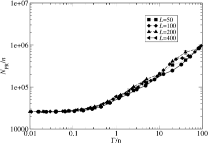
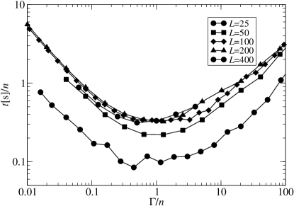
Figure 2: Scaling of PR steps $N_{\mathrm{PR}}$ and CPU time $t$ with system size $n$ for FIFO ($\Delta=2.2$). (a) The average number of PR steps per site, $N_{\mathrm{PR}}/n$, as a function of number of push-relabel steps per site per global update, $\Gamma/n$. The data collapse is consistent with the number of operations scaling with $n$ (the best that can be expected for $\xi\ll L$). (b) CPU time $t$ per site ($t/n$) vs. $\Gamma/n$. The values along both axes have been divided by $n$ the number of sites. A fair collapse develops for $L\geq 100$. The minimum is at $\Gamma_{{\rm min}}/n\approx 1$, independent of system size. The minimum is shallow, however, and even missing $\Gamma_{{\rm min}}$ by a factor of ten increases the running time only by a factor of about two.

IV.1.2 Detailed look at the FIFO data

While determining the optimal global update interval for the FIFO structure, we noticed two features of interest in the data. These features are the tendency for $N_{\mathrm{PR}}$ to be an integer multiple of $\Gamma$ and, at small $\Delta$, a separation of the mean run times between positively and negatively magnetized samples.

A close look at the data reveals piecewise linear behavior in the average running time of the algorithm, when measured by $N_{\mathrm{PR}}$, as displayed in Fig. 3. These linear regions are consistent with $N_{\mathrm{PR}}=k\Gamma$, for integer $k$, as shown by the dashed lines in the figure. These linear regions coincide with plateaus in the number of global updates executed during the solution, $N_{G}$, when plotted vs. $\Gamma$ (see the inset in Fig. 3). The plateaus in $N_{G}$ vs. $\Gamma$ reflect the effect of the global update, which causes large changes in the height field and can bring the auxiliary fields close to a solution. Note that a ground state is found by the algorithm when all of the positive excess is confined to regions that are isolated from sinks. This isolation is due to saturated bonds that block the rearrangement of flow (and to the cancellation of positive excess with negative excess in regions accessible to the sinks). The algorithm will not terminate until the blocked-off regions have their heights raised to $u_{i}=n$. Without global updates ($\Gamma=\infty$), there is a separation between the times when the push-relabel operations effectively determine the domain boundaries by saturating the appropriate bonds and the time when the relabel operations identify the up-spin regions. When $\Gamma$ is finite, but larger than the number of PR steps needed to find all of the domain boundaries and smaller than the total number of PR steps needed to terminate the algorithm, the first global update effectively terminates the running of the algorithm and $N_{G}=1$. There is another interval at smaller values of $\Gamma$ where one global update is executed before the domain boundaries are determined and the second global update terminates the algorithm, giving $N_{G}=2$. This pattern continues to higher values of $m$. We emphasize that the data presented is averaged over $100$ samples at each value of $\Gamma$; the data therefore indicates that the fluctuations in the locations of the linear regions are quite small.

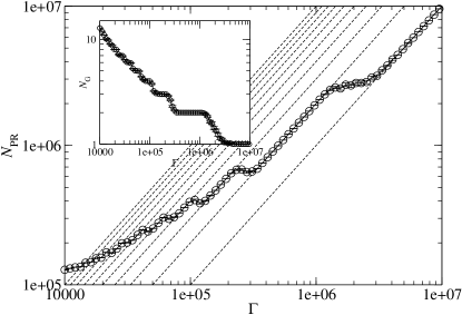
Figure 3: Plot showing the piecewise linear behavior of $N_{\mathrm{PR}}$, the mean number of PR steps needed to find the ground state, when plotted as a function of $\Gamma$, the interval between global updates, for FIFO in $d=2$. The parameter values are $L=200$ and $\Delta=2.2$ and the data is averaged over 100 samples. $N_{\mathrm{PR}}$ increases linearly over intervals in $\Gamma$, $N_{\mathrm{PR}}=k\Gamma$, with the curves for $k=1,2,3,\ldots$ indicated by the dashed lines. The large changes caused by the global update operation can lead to plateaus in the number of global updates $N_{G}$ vs. $\Gamma$, as shown in the inset.

We also noted a strong up-down asymmetry in the running time at small $\Delta$. For $\Delta\ll\Delta_{x}$ and $\Gamma=n$, it takes about 50% longer to find the solution if the ground state is spin-up than if it is spin-down. For $\Gamma\rightarrow\infty$ the ratio of mean running times becomes very large. At small $\Delta$, the ground state is determined by the sum over all random fields. If the sum is negative, the algorithm is done as soon as all the positive excess fields have been annihilated, but if the sum is positive all the sites with remaining excess fields must be moved up to height $n$ before they are labeled inaccessible. This local relabeling can take of the order of $n^{2}$ steps, as essentially each site must be moved stepwise to the maximal height. When a global update is included, the height label of all sites is set to its maximum value once no more sites with negative excess exist. As the global relabeling takes only of the order of $n$ steps, this makes the running times for up- and down- magnetized samples more similar, to within $O(n)$ in total magnitude, for $\Gamma=O(n)$.

IV.1.3 Global update interval for HPQ

For $\Delta<\Delta_{x}$, the behavior of the timing for HPQ vs. $\Gamma$ is very similar to the behavior of the timing for FIFO, with $\Gamma_{{\rm opt}}\approx n$. In contrast, in the paramagnetic regime, gap relabeling detects enclosed domains efficiently and quickly reduces the number of active sites. For large $\Delta$, then, frequent global updates ($\Gamma<n)$ quickly dominate the running time $t$. For $\Gamma>n$, $t$ becomes independent of $\Gamma$ (Fig. 4), as global updates are not executed before the solution is found.

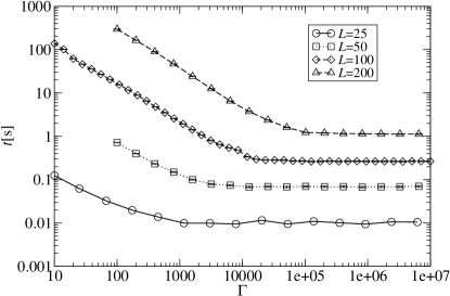
Figure 4: CPU time $t[\textrm{s}]$ for HPQ with gap relabeling vs. $\Gamma$ for $\Delta=2.2>\Delta_{x}$. In this regime gap relabeling is effective and global updates are almost unnecessary. For $\Gamma<n$, the running time increases due to frequent global updates. For $\Gamma>n$, the running time stays constant. There is no discernible minimum in the $t$ vs. $\Gamma$ curve, but $\Gamma=n$ does not hurt performance at large $\Delta$ and improves performance for smaller $\Delta$.

Consistent with the optimal behavior for small $\Delta$ and the independence of $t$ from $\Gamma$ at large $\Delta$, we will use $\Gamma_{{\rm opt}}\approx n$ for the HPQ structure. As $\Gamma=\infty$ is a reasonable choice for larger $\Delta$, we will sometimes include this choice for comparison.

IV.2 FIFO vs. HPQ in two dimensions

Now that we have found an optimal value for $\Gamma$ for each data structure, we can directly compare the performance of FIFO and HPQ for various $\Delta$. We compare timings using $\Gamma=n$ for FIFO and both $\Gamma=n$ and $\Gamma=\infty$ for HPQ. We will refer to the latter two choices as HPQ_n and HPQ_∞, respectively. We computed the mean values of $t$ and $N_{\mathrm{PR}}$ for a large range of system sizes and disorders. The running times were averaged over at least 100 (sometimes as many as $10^{5}$) samples, chosen independently for each value of $L$ and $\Gamma$.

Fig. 5 displays the running time per spin for FIFO with $\Gamma=n$ and Fig. 6 presents a comparison of all three combinations for $L=100$.

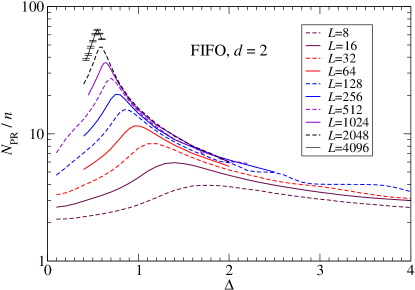
Figure 5: [Color online] Number of push-relabel operations per site needed to solve for the ground state, $N_{\mathrm{PR}}/n$, plotted as a function of $\Delta$, for a 2D square lattice with Gaussian disorder. The number of spins $n=L^{2}$ ranges from $8^{2}$ to $4096^{2}$. Due to the large range of system sizes and hence running times, we have used a logarithmic axis for plotting $N_{\mathrm{PR}}/n$. Statistical error bars and individual points are not displayed, as the point spacing is small and the statistical uncertainties are very small, except for $L=4096$. The global update interval used was $\Gamma=n$. Plateaus are seen when $N_{\mathrm{PR}}$ is close to a multiple of $\Gamma$, especially at larger $\Delta$. Each curve show a pronounced peak, which can be used to define $\Delta_{x}(L)$. At this value of $\Delta,$ the correlation length is of the order of the system size and the system crosses over from a ferromagnetic regime with one large domain to a paramagnetic regime where the correlation length is smaller than the system size. The crossover field $\Delta_{x}$ approaches zero as L goes to infinity, but the approach is logarithmically slow.

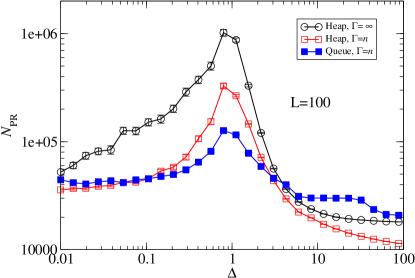
Figure 6: [Color online] Number of PR steps $N_{\mathrm{PR}}$ in $d=2$ for $L=100$. This plot shows the timing for HPQ with ($\Gamma=n$) and without ($\Gamma=\infty$) global updates, compared with FIFO. Note the significant improvement the global update gives to HPQ for field strengths below and at the finite-size crossover.FIFO needs fewer push operations than HPQ_Γ=∞ over almost 3 orders of magnitude in $\Delta$. This difference becomes more pronounced as the system size increases.

The first notable feature in the data is that all three combinations show a pronounced peak in $N_{\mathrm{PR}}$ at a value of $\Delta_{x}(L)$ between 0.5 and 2.0 over the range $L=8$ to $4096$. This peak is reminiscent of the critical slowing down near a phase transition. It moves slowly to the left with increasing system size (Fig. 5), consistent with $\Delta_{x}(L)$ decaying with increasing $L$. As noted in Sec. II, there is no phase transition in 2D, but there is a crossover for any finite size system from a ferromagnetic regime at low $\Delta$ to a paramagnetic regime at large $\Delta$ as the correlation length becomes smaller than the system size.

For small $\Delta$, HPQ_n and FIFO perform very similarly. HPQ_∞, on the other hand, is 2 to 4 times slower in this regime. Near the crossover, the running times for HPQ_n and FIFO start to deviate and the difference is largest at $\Delta_{x}$, where HPQ_n is about 3 times slower than FIFO and HPQ_∞ is yet another factor of 3 slower than HPQ_n.

For $\Delta>\Delta_{x}$, FIFO starts to lose its advantage as domain sizes become smaller and gap relabeling becomes more and more effective with increasing $\Delta$. When $\Delta\approx 3$, HPQ_n starts to outperform FIFO; when $\Delta\approx 20$, FIFO takes twice as many push operations as HPQ_n.

IV.3 Timings for the double Queue (DFIFO)

Our method for simultaneously rearranging both positive and negative excess, DFIFO, performs well for small $\Delta$ in $d=2$ but never better than FIFO. For large values of $\Delta$, it is much slower than FIFO and HPQ. DFIFO performs even worse in 3D. The reason became clear when we visualized the rearrangements of excess field. The visualization shows that positive and negative excesses tend to miss each other. The potential landscape, given by the two height fields, is not updated when excess is pushed and is not consistently updated by relabels. The rearrangement of excess is generally guided by the last global update: the negative excess is pushed to where the positive excess was at the time of the last global update, and vice versa. This lack of coordination between the two height fields becomes more pronounced in higher dimensions, where there are more possible paths between sites. It is possible that using some other combination of the height fields for a heuristic would produce better results. One alternative, for example, would be to combine the separate height fields for positive and negative excesses into a single field. Positive excess would move down the height field gradient and negative excesses would move up the same gradient.

IV.4 Results for three dimensions ($d=3$)

In three dimensions, $\Gamma=n$ remains a good choice for both FIFO and HPQ. As in the case $d=2$, due to a very broad minimum in the dependence of $t$ on $\Gamma$, the exact value of $\Gamma$ is not critical. This is in agreement with previous results where $\Gamma_{\mathrm{min}}=n$ has been found to be a good choice for a variety of sparse and dense graphs Cherkassky and Goldberg (1997a).

The peak in the timing of the algorithm is quite pronounced, as in the 2D data, but in this case the location of the peak converges to a fixed value at large $L$. We gathered data for the number of push-relabel operations $N_{\mathrm{PR}}$ per site, $N_{\mathrm{PR}}/n$, vs. $\Delta$, for sizes $L$ ranging from 8 to 128 for HPQ and LPQ and up to size 256 for the FIFO data structure. The plot of the FIFO data (Fig. 7) shows a growth in $N_{\mathrm{PR}}/n$ with $L$ and convergence to a well-defined curve for the running time for $\Delta$ in the paramagnetic range. In the ferromagnetic regime, there is a slow growth of the running time with sample dimension $L$. Both the LPQ and HPQ data structures are significantly slower than the FIFO data structure, at moderate values of $\Delta$ (with a ratio of $\approx 3$ for the peak running times at $L=128$), as seen in Fig. 8. The LPQ data structure is significantly faster than the HPQ structure on the paramagnetic side of the peak in the running time, but is very similar in speed on the ferromagnetic side. The running time for LPQ converges much more quickly than the HPQ version to an $L$-dependent value as $L$ is increased at fixed $\Delta>\Delta_{c}$.

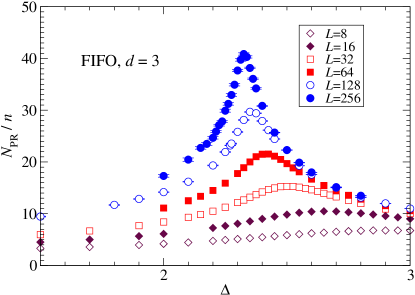
Figure 7: [Color online] Push-relabel operations (cycles) per site, $N_{\mathrm{PR}}/n$, plotted vs. disorder strength $\Delta$ in $d=3$, for $L=8$, 16, 32, 64, 128, and 256, for the push-relabel algorithm using the FIFO data structure. The global update interval is fixed at $\Gamma=n$. There is a clear peak in the running time near $\Delta\approx 2.3$, which is in good agreement with the critical field $\Delta_{c}=2.270(5)$ found Middleton and Fisher (2002) for the ferro- to paramagnetic phase transition for a Gaussian distribution.

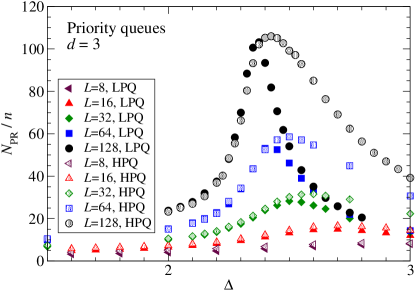
Figure 8: [Color online] Push-relabel operations (cycles) per site $N_{\mathrm{PR}}/n$ vs. $\Delta$ in $d=3$, for $L=8$, 16, 32, 64, 128, and 256, when using the HPQ and LPQ data structures. There is again a clear peak in the running time near $\Delta\approx 2.3$, but the peak is significantly broader and higher for HPQ, than for LPQ. Note that the number of cycles grows more quickly with $L$ than for the FIFO structure.

V Qualitative Description

In order to better understand the timing results, we have visualized the evolution of the height fields and the rearrangement of excess. The visualization code Hambrick (2003) uses a color map to display the height field. The program has the option to display the location of sites with excess (white for positive and black for negative) and to indicate where the flow is saturated, i.e., where $r_{ij}=0$. A sample snapshot from the simulation with both of these options activated is shown in Fig. 9.

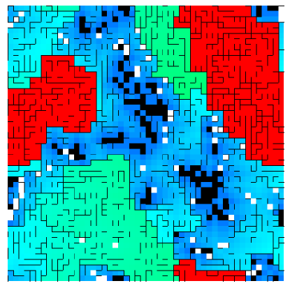
Figure 9: [Color online] Image of the state of the auxiliary fields during the solution of a 2D RFIM of size $L=50$ and with disorder strength $\Delta=2$. This picture shows a snapshot of the height field $u_{i}$, the location of non-zero excess $e(i)$, and bonds with zero residual strength ($r_{ij}=0$), while executing the push-relabel algorithm (HPQ data structure). The red (darkest non-black) regions have already been identified as up; the heights in this region have the maximal value $n=2500$. The colors that are not black or white correspond to the height field in the remainder of the sample: blue (darker colors) indicates a low, while green (lighter colors) indicates a high height. The white squares represent spins with a positive excess field (the height at these sites is not indicated); black squares represent spins with a negative excess (and have height zero). The black lines are dual to the bonds that are saturated (i.e., have zero residual strength). These saturated dual bonds ($r_{ij}=0$ or $r_{ji}=0$) “block” the rearrangement of excess $e_{i}$. More up-spin regions may be identified as more bonds are saturated and the dual bonds link up to isolate a region. The algorithm terminates when all positive excess is confined to up-spin regions.

When $\Delta$ is somewhat larger than $\Delta_{x}$ in $d=2$, the differences between the temporal progress using the HPQ and FIFO data structures are clearly seen in the dynamic visualization. As FIFO cycles through all active sites, all the positive excesses move at a roughly uniform speed down the height gradients. The utility of the global update at late times for FIFO is apparent: when $\Gamma$ is large (infrequent global updates), a few positive excesses are seen to skate around in regions contained by saturated bonds. The pushes have found the minimum cut by saturating the bonds that separate the positive and negative spin regions, but the algorithm hasn’t confirmed that fact yet. The local relabels, which tend to raise a site’s height only by one step at a time, are inefficient in raising a large up-spin domain to maximal height. The remaining positive excesses are shuffled around within the domain, slowly increasing the height by small relabels. When global updates are infrequent, the algorithm may terminate by a final global update, which finds that a set of positive excesses is isolated from all sinks. This confirms the picture discussed in Sec IV.1.2. HPQ, on the other hand, tends to act repeatedly on the same site. Isolated regions with positive excess are raised uniformly above the rest of the sample. This allows the gap heuristic to quickly identify isolated positive spin domains, even when $\Gamma$ is large.

For samples with weak disorder, the algorithm with the HPQ data structure does lead to a few positive excesses racing around the network while the others sit idly. The time to raise a large positive domain high enough to create a gap is large. Again, active sites tend to move around quite a bit, while other regions remain unchanged. Towards the middle of the algorithm execution, the lattice often displays lines or rings of positive excess sitting on an equipotential line near a sink, often immediately adjacent to it. These structures are at low height and cannot move until all excesses of greater height have been removed. This should slow the algorithm down. The positive excesses do not “screen” the sinks, since the global update doesn’t differentiate between sinks of different capacity. This expectation is consistent with our results for the LPQ, which performs somewhat better than HPQ, especially at higher field strengths.

At large field strengths, the proportion of active sites whose random field strength is greater than the strength of their bonds to neighbors (i.e., $\Delta>4$ in 2D) is large. The algorithm acts on most sites only twice. One can clearly see how HPQ sweeps the lattice and raises (nearly) all the sites of initial height two (those with no adjacent sinks) to the maximum height, then does the same to sites of height one. FIFO also generally makes two or three passes, though its first pass executes pushes on the sites where pushing is possible and relabels otherwise.

VI Summary

As has been demonstrated before Bastea and Duxbury (1998); Duxbury and Meinke (2001); Esser et al. (1997); Hartmann (1998); Hartmann and Nowak (1998); Middleton and Fisher (2002); Ogielski (1986); Seppälä (1996), the PR algorithm is an efficient method to find the exact ground state for the RFIM at T=0 in any dimension. Here we investigated how to implement PR to find the ground state most quickly. We compared a number of data structures and the effect of global and gap relabeling on the performance of the algorithm.

In agreement with previous work Seppälä (1996), our detailed results recommend the FIFO-queue combined with global updates every $\Gamma\approx kn$ steps, with $k$ a number near unity. FIFO performs much better near the crossover disorder ($\Delta_{x}$ for $d=1,2$) and the critical disorder ($\Delta_{c}$ in $d=3$) and never performs significantly worse than HPQ. The exact value of $\Gamma$ is not crucial since the minimum in $t$ vs. $\Gamma$ is very broad.

We also tried an implementation that treats positive and negative excesses equally. This implementation, however, suffers from the lack of coordination between the height fields for the two sets of excesses and positive and negative excesses tend to miss each other. It is likely that this algorithm could be improved by using a single height field to coordinate the motion of the positive and negative excess.

A more flexible approach to the global update interval might also be useful in speeding up simulations. It is likely that adaptively modifying the global updates so that they are executed when the sink density changes by a defined fraction or packets of excess have travelled a given distance would optimize the algorithm during each stage of the solution. There is still a lot of room for other modification, e.g., cutting off the breadth first search to reflect saturation and non-uniform intervals for global update that depend on the number of sinks that have been annihilated since the last global update rather than the number of PR steps.

We found that the visualization of the operations (see Hambrick (2003) for the source code) greatly improved our understanding of the algorithm. This code may be useful in suggesting further improvements to the algorithm.