Universal scaling behavior
of non-equilibrium phase transitions

Summary

Non-equilibrium critical phenomena have attracted a lot of research interest in the recent decades. Similar to equilibrium critical phenomena, the concept of universality remains the major tool to order the great variety of non-equilibrium phase transitions systematically. All systems belonging to a given universality class share the same set of critical exponents, and certain scaling functions become identical near the critical point. It is known that the scaling functions vary more widely between different universality classes than the exponents. Thus, universal scaling functions offer a sensitive and accurate test for a system’s universality class. On the other hand, universal scaling functions demonstrate the robustness of a given universality class impressively. Unfortunately, most studies focus on the determination of the critical exponents, neglecting the universal scaling functions.

In this work a particular class of non-equilibrium critical phenomena is considered, the so-called absorbing phase transitions. Absorbing phase transitions are expected to occur in physical, chemical as well as biological systems, and a detailed introduction is presented. The universal scaling behavior of two different universality classes is analyzed in detail, namely the directed percolation and the Manna universality class. Especially, directed percolation is the most common universality class of absorbing phase transitions. The presented picture gallery of universal scaling functions includes steady state, dynamical as well as finite size scaling functions. In particular, the effect of an external field conjugated to the order parameter is investigated. Incorporating the conjugated field, it is possible to determine the equation of state, the susceptibility, and to perform a modified finite-size scaling analysis appropriate for absorbing phase transitions. Focusing on these equations, the obtained results can be applied to other non-equilibrium continuous phase transitions observed in numerical simulations or experiments. Thus, we think that the presented picture gallery of universal scaling functions is valuable for future work.

Additionally to the manifestation of universality classes, universal scaling functions are useful in order to check renormalization group results quantitatively. Since the renormalization group theory is the basis of our understanding of critical phenomena, it is of fundamental interest to examine the accuracy of the obtained results. Due to the continuing improvement of computer hardware, accurate numerical data have become available, resulting in a fruitful interplay between numerical investigations and renormalization group analyzes.

Contents

toc

Chapter 1 Introduction

1.1 Opening remarks and outline

One of the most impressive features of continuous phase transitions is the concept of universality, that allows to group the great variety of different critical phenomena into a small number of universality classes (see [1] for a recent review). All systems belonging to a given universality class have the same critical exponents, and certain scaling functions (equation of state, correlation functions, etc.) become identical near the critical point. The universality has its origin in the long range character of the fluctuations. Close to the transition point, the corresponding correlation length becomes much larger than the typical range of molecular interactions. Then the behavior of the cooperative phenomena becomes independent of the microscopic details of the considered system. The concept of universality is well established for equilibrium phase transitions where a unifying theoretical framework exists. In that case, the universal behavior of short-range interacting systems depends only on few fundamental parameters, namely the dimensionality of space and the symmetry of the order parameter [2]. Classical examples of such universal behavior in critical equilibrium systems are for instance the coexistence curve of liquid-vapor systems [3] and the equation of state in ferromagnetic systems (e.g. [1, 4]). A complete understanding of the critical behavior of a given system would require to calculate the critical exponents and the universal scaling functions exactly. In general, this is only possible above the upper critical dimension where mean field theories apply. But the universality ensures that even rather crude modeling of complicated microscopic behavior provides quantitatively many essential features of the critical behavior. Therefore, highly accurate estimates of critical exponents of various universality classes are known (see e.g. [5]).

In contrast to equilibrium critical phenomena, less is known in case of non-equilibrium phase transitions. Here, a generalized treatment is not known, lacking an analog to the equilibrium free energy. Thus the rich and often surprising variety of non-equilibrium phase transitions (see for example [6, 7, 8, 9, 10]) observed in physical, chemical, biological, as well as socioeconomic systems, has to be studied for each system individually. But similar to equilibrium systems it is believed that non-equilibrium critical phenomena can be grouped into universality classes and the concept of universality plays again a central role in theoretical and numerical analysis. The universality implies in turn that oversimplified representations or caricatures of nature provide quantitatively correct results, if the essential features are captured which are responsible for non-equilibrium ordering. Partial differential equations as well as interacting lattice models are two established approaches to study non-equilibrium systems. In the first case a set of partial differential equations is usually constructed on a mean field level by directly translating the reaction scheme (e.g. of a chemical reaction) into equations for gain and loss of certain quantities. The typically non-linear dynamics is described by deterministic equations, and phase transitions are related to bifurcations [6]. Adding suitably chosen noise functions, improved results can be obtained within a Langevin approach or a Fokker-Planck description (see e.g. [11, 12]). In that case, field theoretical approaches assisted by renormalization group techniques are successfully applied to obtain results beyond the mean field level. On the other hand, microscopic interacting particle systems like lattice-gas models or cellular automata [13] provide another insight into non-equilibrium critical phenomena. Although an exciting development has been seen in the last decade leading to a series of exact solutions of interacting particle systems (see e.g. [14]), most models are not accessible to exact mathematical treatment, in particular in higher than one dimension. Thus numerical simulations on increasingly powerful computers are widely used in order to obtain quantitative results.

As pointed out, a full classification of the universality classes of non-equilibrium phase transitions is still lacking, i.e., neither the universality classes nor their defining fundamental parameters are known. Therefore, numerous (mostly phenomenologically motivated) classifications schemes are discussed in the literature. These universality hypotheses have to be checked model by model. Due to a lack of analytical solutions, numerical simulations or renormalization group treatments are used (often in a fruitful interplay) to identify a system’s critical behavior, i.e., to specify the order parameter, predicting the order of the transition, and describing the scaling behavior in the vicinity of the transition point via critical exponents and scaling functions. Unfortunately, most work focuses on the determination of the critical exponents only, neglecting the determination of the universal scaling functions. It turns out that checking the universality class it is often a more exact test to consider scaling functions rather than the values of the critical exponents. While for the latter ones the variations between different universality classes are often small, the scaling functions may differ significantly. Thus the agreement of universal scaling functions provides not only additional but also independent and more convincing evidence in favor of the conjecture that the phase transitions of two models belong to the same universality class.

It is the aim of this work to demonstrate the usefulness of universal scaling functions for the analysis of non-equilibrium phase transitions. In order to limit the coverage of this article, we do not present an overview of non-equilibrium phase transitions as it was done for example in recent review articles [7, 8]. Instead we focus on a particular class of non-equilibrium critical phenomena, the so-called absorbing phase transitions. These phase transitions arise from a competition of opposing processes, usually creation and annihilation processes. The transition point separates an active phase and an absorbing phase in which the dynamics is frozen. A systematic analysis of universal scaling functions of absorbing phase transitions is presented, including static, dynamical, and finite-size scaling measurements. As a result a picture gallery of universal scaling functions is presented which allows to identify and to distinguish universality classes.

The outline of this work is as follows: in the remaining part of the introduction a transparent formulation of scaling and universality is presented, since both notions are central to the understanding of critical phenomena. Therefore, we follow the historic perspective and survey phenomenologically the basic ideas of equilibrium critical phenomena, and discuss the concepts of critical exponents, generalized homogenous functions, scaling forms, as well as universal amplitude combinations. A foundation for an understanding of scaling and universality is provided by Wilson’s renormalization group theory [15, 16], which is a topic on its own and not presented in this work. Instead we focus on the implications on universal scaling and just illustrate the main results, e.g. we sketch how the renormalization group theory allows to decide on the relevant system parameters determining the universality class. The renormalization group also provides a tool for computing critical exponents as well as the universal scaling functions, and it explains the existence of an upper critical dimension. For a rigorous substantiation of scaling and universality the interested reader is referred to established textbooks (e.g. [17, 18, 19]) and review articles [20, 21, 22]. While we have attempted to present the introduction as general as possible, we use for the sake of concreteness the language of ferromagnetic phase transitions. In conclusion, the subsequent sections can be used as an introduction to the theory of phase transitions for readers unfamiliar with the concepts of scaling and universality. Readers familiar with equilibrium critical phenomena and interested in non-equilibrium systems are recommended to skip the introduction.

In chapter 2 we introduce the definitions and notations of absorbing phase transitions. To be specific, we present a mean field treatment of the contact process providing a qualitative but instructive insight. Various simulation techniques are discussed for both steady state and dynamical measurements. In particular, the mean field results are compared briefly to those obtained from simulations of the high-dimensional contact process. The chapters 3 and 4 are devoted to the investigation of two different universality classes: the directed percolation universality class and the so-called Manna universality class. According to its robustness and ubiquity the universality class of directed percolation (DP) is recognized as the paradigm of the critical behavior of several non-equilibrium systems exhibiting a continuous phase transition from an active to an absorbing state. The widespread occurrence of such models describing critical phenomena in physics, biology, as well as catalytic chemical reactions is reflected by the universality hypothesis of Janssen and Grassberger: Short-range interacting models, which exhibit a continuous phase transition into a unique absorbing state, belong to the directed percolation universality class, provided they are characterized by a one-component order parameter [23, 24]. Different universality classes are expected to occur e.g. in the presence of additional symmetries or quenched disorder. The universality class of directed percolation is well understood. In particular, a field theoretical description is well established, and renormalization group treatments provide within an $\epsilon$-expansion useful estimates of both the critical exponents and the scaling functions. But it should be remembered that the renormalization group rarely provides exact results, i.e., it is essential to have an independent (usually numerical or experimental) check. These checks are of fundamental interest since the renormalization group theory is the basis of our understanding of critical phenomena. Remarkably, a detailed analysis shows that renormalization group approximations reveals more accurate results for directed percolation than for standard equilibrium models. In contrast to directed percolation, less is known in case of the Manna universality class. For example, field theoretical approaches using renormalization group techniques run into difficulties. Thus a systematic $\epsilon$-expansion is still lacking, and most quantitative results are obtained from numerical simulations. The Manna universality class is of particular interest since it is related to the concept of self-organized criticality.

For both universality classes considered several lattice models are investigated. A systematic analysis of certain scaling functions below, above as well as at the upper critical dimension is presented. At the upper critical dimension, the usual power-law behavior is modified by logarithmic corrections. These logarithmic corrections are well known for equilibrium critical phenomena, but they have been largely ignored for non-equilibrium phase transitions. Due to the considerably high numerical effort, sufficiently accurate simulation data have become available recently, triggering further renormalization group calculations and vice versa. The results indicate that the scaling behavior can be described in terms of universal scaling functions even at the upper critical dimension. Independent of the dimension, we investigate steady state scaling functions, dynamical scaling functions, as well as finite-size scaling functions. Focusing on common scaling functions such as the equation of state our method of analysis can be applied to other non-equilibrium continuous phase transitions observed numerically or experimentally. Thus we hope that the presented gallery of universal scaling functions will be useful for future work where the scaling behavior of a given system has to be identified. Additionally, certain universal amplitude combinations are considered. In general, universal amplitude combinations are related to particular values of the scaling functions. Systematic approximations of these amplitude combinations are often provided by renormalization group treatments. Furthermore, the validity of certain scaling laws connecting the critical exponents is tested.

Crossover phenomena between different universality classes are considered in chapter 5. Although crossover phenomena are well understood in terms of competing fixed points, several aspects are still open and are discussed in the literature. For example, the question whether the full crossover region, that spans usually several decades in temperature or conjugated field, can be described in terms of universal scaling functions attracted a lot of research activity. Here, we consider several models belonging to the Manna universality class with various interaction range. Our analysis reveals that the corresponding crossover from mean field to non-mean field scaling behavior can be described in terms of universal scaling functions. This result can be applied to continuous phase transitions in general, including equilibrium crossover phenomena.

Concluding remarks are presented in Chapter 6. Furthermore, we direct the reader’s attention to areas where further research is desirable. The work ends with appendices containing tables of critical exponents as well as universal amplitude combinations.

A comment is worth making in order to avoid confusion about the mathematical notation of asymptotical scaling behavior. Throughout this work the Landau notation [25, 26] is used, i.e., the symbols $\,\propto\,$, $\,\sim\,$, and $\mathcal{O}$ denote that two functions $f(x)$ and $g(x)$ are

$$\begin{array}[]{llll}f(x)\propto g(x)&\Longleftrightarrow&\frac{\displaystyle f(x)}{\,\displaystyle g(x)^{\vphantom{X}}\,}=c\,,\quad\forall\,x&\quad\mathrm{(proportional)}\,,\\[11.38109pt] f(x)=g(x)+\mathcal{O}(x^{n})&\Longleftrightarrow&\left|\frac{\displaystyle\,f(x)-g(x)\,}{\displaystyle x^{n\vphantom{X}}}\right|<c\,,\forall\,x>x_{\scriptscriptstyle 0}&\quad\mathrm{(of\;the\;order\;of)},\\[11.38109pt] f(x)\sim g(x)&\Longleftrightarrow&\lim\limits_{\scriptscriptstyle x\to x_{\mathrm{c}}}\frac{\displaystyle f(x)}{\displaystyle\,g(x)^{\vphantom{X}}\,}=1&\quad\mathrm{(asymptotically\;equal)}\,.\end{array}$$

In the following, the mathematical limit $x\to x_{\scriptscriptstyle{\mathrm{c}}}$ corresponds to the physical situation that a phase transition is approached (usually $x\to 0$ or $x\to\infty$). Beyond this standard notation the symbol $\,\,{\tilde{\propto}}\,\,$ is used to denote that the functions are asymptotically proportional, i.e.,

$$f(x)\,{\tilde{\propto}}\,g(x) \Longleftrightarrow \lim_{\scriptscriptstyle x\to x_{\mathrm{c}}}\frac{f(x)}{\,g(x)^{\vphantom{X}}\,}=c\quad\quad\quad\;\;\,\mathrm{(asymptotically\;proportional)}.$$

1.2 Scaling theory

Phase transitions in equilibrium systems are characterized by a singularity in the free energy and its derivatives [27, 28, 29]. This singularity causes a discontinuous behavior of various physical quantities when the transition point is approached. Phenomenologically the phase transition is described by an order parameter, having non-zero value in the ordered phase and zero value in the disordered phase [30]. Prototype systems for equilibrium phase transitions are simple ferromagnets, superconductors, liquid-gas systems, ferroelectrics, as well as systems exhibiting superfluidity.

In case of ferromagnetic systems the transition point separates the ferromagnetic phase with non-zero magnetization from the paramagnetic phase with zero magnetization. The well-known phase diagram is shown in Figure 1. Due to the reversal symmetry of ferromagnets all transitions occur at zero external field $h$. The phase diagram exhibits a boundary line along the temperature axis, terminating at the critical point $T_{\scriptscriptstyle\mathrm{c}}$. Crossing the boundary for $T<T_{\scriptscriptstyle\mathrm{c}}$ the magnetization changes discontinuously, i.e. the systems undergoes a first order phase transition. The discontinuity decreases if one approaches the critical temperature. At $T_{\scriptscriptstyle\mathrm{c}}$ the magnetization is continuous but its derivatives are discontinuous. Here the system undergoes a continuous or so-called second order phase transition. For $T>T_{\scriptscriptstyle\mathrm{c}}$ no singularities of the free energy occur and the systems changes continuously from a state of positive magnetization to a state of negative magnetization.

In zero field the high temperature or paramagnetic phase is characterized by a vanishing magnetization. Decreasing the temperature, a phase transition takes place at the critical temperature and for $T<T_{\scriptscriptstyle\mathrm{c}}$ one observes an ordered phase which is spontaneously magnetized (see Figure 1). Following Landau, the magnetization $m$ is the order parameter of the ferromagnetic phase transition [30]. Furthermore the temperature $T$ is the control parameter of the phase transition and the external field $h$ is conjugated to the order parameter. As well known, critical systems are characterized by power-laws sufficiently close to the critical point, e.g. the behavior of the order parameter can be described by

$$m(T,h=0)\;\,{\tilde{\propto}}\,\;(-\delta T)^{\beta}$$ (1.1)

with the reduced temperature $\delta T=(T-T_{\scriptscriptstyle\mathrm{c}})/T_{\scriptscriptstyle\mathrm{c}}$ and the exponent $\beta$.

Figure 1: Sketch of the ferromagnetic phase diagram (left) and the corresponding order parameter behavior (right). The phase diagram contains a line of first-order transitions at zero field (dashed line) that ends in a critical point at temperature $T_{\scriptscriptstyle\mathrm{c}}$. The temperature dependence of the magnetization is sketched for zero-field (thick line) and three different values of the conjugated field.

For non-zero field the magnetization increases smoothly with decreasing temperature. At the critical isotherm ($\delta T=0$) the magnetization obeys another power-law for $h\to 0$

$$m(T=T_{\scriptscriptstyle\mathrm{c}},h)\;\,{\tilde{\propto}}\,\;|h|^{1/\delta}\,.$$ (1.2)

Further exponents are introduced to describe the singularities of the order parameter susceptibility $\chi$, the specific heat $C$, as well as the correlation length $\xi$

$$\chi(T,h=0) \,{\tilde{\propto}}\, |\delta T|^{-\gamma}\,,$$ (1.3)

$$C(T,h=0) \,{\tilde{\propto}}\, |\delta T|^{-\alpha}\,,$$ (1.4)

$$\xi(T,h=0) \,{\tilde{\propto}}\, |\delta T|^{-\nu}\,.$$ (1.5)

Another exponent $\eta$ describes the spatial decay of the correlation function at criticality

$$\Gamma(r)\;\,{\tilde{\propto}}\,\;r^{-D+2-\eta}\,,$$ (1.6)

where $D$ denotes the dimensionality of the system.

A comment about vanishing exponents is worth making. A zero exponent corresponds either to a jump of the corresponding quantity at the critical point or to a logarithmic singularity since

$$-\ln{|\delta T|}\;=\;\lim_{s\to 0}{\frac{\,|\delta T|^{-s}-1\,}{s}}\,.$$ (1.7)

Often, it is notoriously difficult to distinguish from experimental or numerical data a logarithmic singularity from a small positive value of the exponent.

The exponents $\alpha$, $\beta$, $\gamma$, $\delta$, $\eta$, and $\nu$ are called critical exponents. Notice in Eqs. (1.3-1.5) the equality of the critical exponents below and above the critical point, which is an assumption of the scaling theory. The phenomenological scaling theory was developed by several authors in the 1960s (e.g. [31, 32, 33, 34, 35, 36]) and has been well verified by experiments as well as simulations. In particular, the scaling theory predicts that the critical exponents mentioned above are connected by the scaling laws

$$\alpha+2\beta+\gamma\;=\;2\quad (\mathrm{Rushbrooke}),$$ (1.8)

$$\gamma\;=\;\beta\,(\delta-1)\quad (\mathrm{Widom}),$$ (1.9)

$$\gamma\;=\;(2-\eta)\,\nu\quad (\mathrm{Fisher}),$$ (1.10)

$$2-\alpha\;=\;\nu\,D\quad (\mathrm{Josephson})\,.$$ (1.11)

The Josephson law includes the spatial dimension $D$ of the system and is often termed the hyperscaling relation. In this way the critical behavior of an equilibrium system is determined by two independent critical exponents.

The scaling theory rests on the assumption that close to the critical point the singular part of a particular thermodynamic potential is asymptotically a generalized homogeneous function (see e.g. [37]). A function $f(x_{\scriptscriptstyle 1},x_{\scriptscriptstyle 2},\ldots)$ is a generalized homogeneous function if it satisfies the following equation for all positive values of $\lambda$

$$\lambda\;f(x_{\scriptscriptstyle 1},x_{\scriptscriptstyle 2}\ldots)\;=\;f(\lambda^{s_{\scriptscriptstyle 1}}x_{\scriptscriptstyle 1},\lambda^{s_{\scriptscriptstyle 2}}x_{\scriptscriptstyle 2},\ldots)\,.$$ (1.12)

The exponents $s_{\scriptscriptstyle 1},s_{\scriptscriptstyle 2},\ldots$ are usually termed scaling powers and the variables $x_{\scriptscriptstyle 1},x_{\scriptscriptstyle 2},\ldots$ are termed the scaling fields. In case of ferromagnetism the singular part of the Gibbs potential per spin $g_{\scriptscriptstyle\mathrm{sing}}(\delta T,h)$ is assumed to scale asymptotically as

$$g_{\scriptscriptstyle\mathrm{sing}}(\delta T,h)\;\sim\;\lambda^{\alpha-2}\;\;{\tilde{g}}(\delta T\,\lambda,h\,\lambda^{\beta\delta})\,,$$ (1.13)

with the scaling function ${\tilde{g}}(x,y)$. The scaling power of the conjugated field is often denoted as the gap-exponent $\Delta=\beta\,\delta$. Strictly speaking, Eq. (1.13) is only asymptotically valid, i.e., only when $\delta T$ and $h$ tend to zero. Corrections occur away from this limit. It turns out that all Legendre transformations of generalized homogenous functions and all partial derivatives of generalized homogenous functions are also generalized homogenous functions. Thus with the Gibbs potential all thermodynamic potentials and all thermodynamic functions that are expressible as derivatives of thermodynamic potentials, like the magnetization, specific heat, etc., are generalized homogeneous functions.

Consider, for example, the magnetization and the corresponding susceptibility. Differentiating Eq. (1.13) with respect to the conjugated field we find

$$m(\delta T,h) = -\left(\frac{\partial\,g_{\scriptscriptstyle\mathrm{sing}}}{\partial\,h}\right)_{T}\;\sim\;\lambda^{\alpha-2+\beta\delta}\;\;{\tilde{m}}(\delta T\,\lambda,h\,\lambda^{\beta\delta})\,,$$ (1.14)

$$\chi(\delta T,h) = -\left(\frac{\partial^{2}\,g_{\scriptscriptstyle\mathrm{sing}}}{\partial\,h^{2}}\right)_{T}\;\sim\;\lambda^{\alpha-2+2\beta\delta}\;\;{\tilde{\chi}}(\delta T\,\lambda,h\,\lambda^{\beta\delta})\,,$$ (1.15)

where the scaling functions are given by

$${\tilde{m}(x,y)}\;=\;-\left(\frac{\partial\,{\tilde{g}}(x,y)}{\partial\,y}\right)_{x}\,,\quad\quad\quad{\tilde{\chi}(x,y)}\;=\;-\left(\frac{\partial^{2}\,{\tilde{g}}(x,y)}{\partial\,y^{2}}\right)_{x}\,.$$ (1.16)

Since the Eqs. (1.14-1.15) are valid for all positive values of $\lambda$ they hold for $\lambda=1/|\delta T|$, hence one obtains at zero-field

$$m(\delta T,0) \sim (-\delta T)^{-(\alpha-2+\beta\delta)}\;\;{\tilde{m}}(-1,0)\,,$$ (1.17)

$$\chi(\delta T,0) \sim |\delta T|^{-(\alpha-2+2\beta\delta)}\;\;{\tilde{\chi}}(\raisebox{0.86108pt}{$\scriptstyle\pm$}1,0)\,,$$ (1.18)

where the magnetization is defined for $\delta T<0$ only. Notice that one expects ${\tilde{\chi}}(+1,0)\neq{\tilde{\chi}}(-1,0)$ in general, i.e., the amplitudes of the susceptibility are different below ($T<T_{\scriptscriptstyle\mathrm{c}}$) and above ($T>T_{\scriptscriptstyle\mathrm{c}}$) the transition. Comparing with Eq. (1.1) and Eq. (1.3) we find

$$\beta\;=\;-\alpha+2-\beta\,\delta\,,\quad\quad\quad\gamma\;=\;\alpha-2+2\,\beta\,\delta\,,$$ (1.19)

which leads directly to the Rushbrook [Eq. (1.8)] and Widom [Eq. (1.9)] scaling law. The Fisher and Josephson scaling laws can be obtained in a similar way from the scaling form of the correlation function (see e.g. [19]). In order to obtain the Josephson law both thermodynamic scaling forms and correlation scaling forms have to be combined. Scaling relations obtained in this way are usually termed hyperscaling laws and do not hold above the upper-critical dimension.

The scaling theory implies still more. Consider for instance the $M$-$h$-$t$ equation of state [Eq. (1.14)]. Choosing $h\lambda^{\beta\delta}=1$ in Eq. (1.14) we find

$$m(\delta T,h)\;\sim\;\left.\lambda^{-\beta}\;\;{\tilde{m}}(\delta T\,\lambda,h\,\lambda^{\beta\delta})\right|_{\lambda=h^{-1\beta\delta}}\;=\;h^{1/\delta}\;\;{\tilde{m}}(\delta T\,h^{-1/\beta\delta},1)\,.$$ (1.20)

At the critical isotherm ($\delta T=0$) we recover Eq. (1.2). Furthermore, the equation of state may be written in the rescaled form

$$m_{\scriptscriptstyle h}\;\sim\;{\tilde{m}}(\delta T_{\scriptscriptstyle h},1)\quad\quad{\mathrm{with}}\quad\quad m_{\scriptscriptstyle h}=m\,h^{-1/\delta}\,,\quad\delta T_{\scriptscriptstyle h}=\delta T\,h^{-1/\beta\delta}\,.$$ (1.21)

In this way the equation of state is described by the single curve ${\tilde{m}}(x,1)$ and all $M$-$h$-$t$ data points will collapse onto the single curve ${\tilde{m}}(x,1)$ if one plots the rescaled order parameter $m_{\scriptscriptstyle h}$ as a function of the rescaled control parameter $\delta T_{\scriptscriptstyle h}$. This data-collapsing is shown in Figure 2 for the magnetization curves of Figure 1.

Figure 2: The data-collapsing of the $M$-$h$-$t$ equation of state. The data correspond to the three different magnetization curves of Figure 1. All data points collapse onto the curves ${\tilde{m}}(x,1)$ (left, Hankey-Stanley scaling form [Eq. (1.21)]) and ${\tilde{h}}(x,1)$ (right, Widom-Griffiths scaling form [Eq. (1.21)]), respectively. The so-called metric factors are defined in section 1.3. The circles mark the normalization conditions Eq. (1.29) and Eq. (1.33).

A different scaling form is obtained if one considers instead of the Gibbs potential the Helmholtz potential $a=g+m\,h$. Since Legendre transforms of generalized homogeneous functions are also generalized homogeneous functions the singular part of the Helmholtz potential obeys

$$a_{\scriptscriptstyle\mathrm{sing}}(\delta T,m)\;\sim\;\lambda^{\alpha-2}\;\;{\tilde{a}}(\delta T\,\lambda,m\,\lambda^{\beta})\,.$$ (1.22)

This equation leads to the scaling form of the conjugated field

$$h(\delta T,m)\;=\;\left(\frac{\partial\,a_{\scriptscriptstyle\mathrm{sing}}}{\partial\,m}\right)_{T}\;\sim\;\lambda^{-\beta\delta}\;\;{\tilde{h}}(\delta T\,\lambda,m\,\lambda^{\beta})\,.$$ (1.23)

Choosing $m\,\lambda^{\beta}=1$ we find

$$h_{\scriptscriptstyle m}\;\sim\;{\tilde{h}}(\delta T_{\scriptscriptstyle m},1)\quad\quad{\mathrm{with}}\quad\quad h_{\scriptscriptstyle m}=h\,m^{-\delta}\,,\quad\delta T_{\scriptscriptstyle m}=\delta T\,m^{-1/\beta}\,.$$ (1.24)

Both, ${\tilde{h}}(x,1)$ and ${\tilde{m}}(x,1)$ are analytic in the neighborhood of $x=0$, i.e., at the critical temperature. The function ${\tilde{h}}(x,1)$ is often called the Widom-Griffiths scaling function [33, 36] whereas we term in the following ${\tilde{m}}(x,1)$ as the Hankey-Stanley scaling function [37]. The corresponding data-collapses for both scaling forms are presented in Figure 2. The Hankey-Stanley scaling form is just the order parameter curve as a function of the control parameter in a fixed conjugated field. It is therefore the natural and perhaps more elegant way to present data-collapses of the equation of state. But often the mathematical forms of the Hankey-Stanley functions are rather complicated whereas the Widom-Griffiths scaling forms are analytically tractable. Therefore ${\tilde{h}}(x,1)$ is often calculated within certain approximation schemes, e.g. $\epsilon$- or $1/n$-expansions within a renormalization group approach.

Notice that the definition of a generalized homogeneous function [Eq. (1.12)] and the data-collapse representations

$$|x_{\scriptscriptstyle 1}|^{-1/s_{\scriptscriptstyle 1}}\;f(x_{\scriptscriptstyle 1},x_{\scriptscriptstyle 2}) = f(\raisebox{0.86108pt}{$\scriptstyle\pm$}1,x_{\scriptscriptstyle 2}\,|x_{\scriptscriptstyle 1}|^{-s_{\scriptscriptstyle 2}/s_{\scriptscriptstyle 1}})\,,$$ (1.25)

$$|x_{\scriptscriptstyle 2}|^{-1/s_{\scriptscriptstyle 2}}\;f(x_{\scriptscriptstyle 1},x_{\scriptscriptstyle 2}) = f(x_{\scriptscriptstyle 1}\,|x_{\scriptscriptstyle 2}|^{-s_{\scriptscriptstyle 1}/s_{\scriptscriptstyle 2}},\raisebox{0.86108pt}{$\scriptstyle\pm$}1)$$ (1.26)

are mathematically equivalent, i.e., a function $f(x_{\scriptscriptstyle 1},x_{\scriptscriptstyle 2})$ is a generalized homogeneous function if and only if Eq. (1.25), or equally Eq. (1.26), is fulfilled [37]. This was important for the phenomenological formulation of the scaling theory since it has been borne and has been confirmed by numerous data-collapses of experimental and numerical data.

1.3 Universality

According to the scaling laws Eqs. (1.8-1.11) equilibrium phase transitions are characterized by two independent critical exponents. In the 1950s and 1960s it was experimentally recognized that quantities like $T_{\scriptscriptstyle\mathrm{c}}$ depend sensitively on the details of the interactions whereas the critical exponents are universal, i.e., they depend only on a small number of general features. This led to the concept of universality which was first clearly phrased by Kadanoff [2], but based on earlier works including e.g. [38, 39, 40, 41, 42]. The universality hypothesis reduces the great variety of critical phenomena to a small number of equivalence classes, so-called universality classes, which depend only on few fundamental parameters. All systems belonging to a given universality class have the same critical exponents and the corresponding scaling functions become identical near the critical point. For short range interacting equilibrium systems the fundamental parameters determining the universality class are the symmetry of the order parameter and the dimensionality of space [2, 41]. The specific nature of the transition, i.e. the details of the interactions, such as the lattice structure and the range of interactions (as long as it remains finite) do not affect the scaling behavior. For instance, ferromagnetic systems with one axis of easy magnetization are characterized by a one component order parameter ($n=1$) and belong to the universality class of the Ising ferromagnet. Furthermore, liquid-gas transitions [43, 44, 45, 46, 47, 48], binary mixtures of liquids [49], and systems exhibiting an order-disorder transition in alloys such as beta-brass are described by a scalar order parameter, too, and belong therefore to the same universality class (see e.g. [50]). Even phase transitions occurring in high-energy physics are expected to belong to the Ising universality class. For example, within the electroweak theory the early universe exhibits a transition from a symmetric (high temperature) phase to a broken so-called Higgs phase [51]. The occurring line of first order phase transitions terminates at a second order point which is argued to belong to the Ising class.

Ferromagnetic systems with a plane of easy magnetization are characterized by a two-component order parameter ($n=2$). Representatives of this universality class are the XY-model, superconductors, as well as liquid crystals that undergo a phase transition from a smectic-A to a nematic phase [52, 53, 54]. But the most impressive prototype is the superfluid transition of ${}^{4}{\mathrm{He}}$ along the $\lambda$-line. Due to its characteristic features like the purity of the samples, the weakness of the singularity in the compressibility of the fluid, as well as the reasonably short thermal relaxation times, superfluid ${}^{4}{\mathrm{He}}$ is more suitable for high-precision experiments than any other system [55]. For example, orbital heat capacity measurements of liquid helium to within $2\,\mathrm{nK}$ from the $\lambda$-transition provide the estimate $\alpha=-0.01285\pm 0.00038$ [56, 57]. Thus, the $\lambda$-transition of ${}^{4}\mathrm{He}$ offers an exceptional opportunity to test theoretical predictions, obtained in particular from renormalization group theory (see e.g. [58] and references therein).

The well known Heisenberg universality class describes isotropic ferromagnetic systems that are characterized by a three component order parameter ($n=3$). Despite of the Ising, XY, and Heisenberg universality classes other classes with $n\hskip 2.15277pt\raisebox{1.72218pt}{$\scriptstyle\geq$}\hskip 2.15277pt4$ are discussed in the literature. For instance, the $n=5$ universality class is expected to be relevant for the description of high-$T_{\scriptscriptstyle\mathrm{c}}$ superconductors [59, 60] whereas $n=18$ is reported in the context of superfluid ${}^{3}{\mathrm{He}}$ [61]. Furthermore, the limit $n\to 0$ corresponds to the critical behavior of polymers and self-avoiding random walks [62]. The other limiting case $n\to\infty$ corresponds to the exactly solvable spherical model [63, 64, 65].

In the scaling theory presented above, the exponents are already universal but the scaling functions are non-universal. Thus two systems are characterized by e.g. two different scaling functions ${\tilde{m}}$ although they are in the same universality class. The non-universal features can be absorbed into two non-universal parameters leading to the universal scaling function ${\tilde{M}}$

$$c_{\scriptscriptstyle m}\,m(\delta T,h)\;\sim\;\lambda^{-\beta}\;\;{\tilde{M}}(c_{\scriptscriptstyle T}\delta T\,\lambda,c_{\scriptscriptstyle h}h\,\lambda^{\beta\delta})\,.$$ (1.27)

In this way, the universal scaling function ${\tilde{M}}$ is the same for all models belonging to a given universality class whereas all non-universal system-dependent features are contained in the metric factors $c_{\scriptscriptstyle m}$, $c_{\scriptscriptstyle T}$, and $c_{\scriptscriptstyle h}$ [66]. Since this scaling form is valid for all positive values of $\lambda$, the number of metric factors can be reduced by a simple transformation. For the sake of convenience we choose $c_{\scriptscriptstyle m}^{1/\beta}\lambda\mapsto\lambda$, yielding

$$m(\delta T,h)\;\sim\;\lambda^{-\beta}\;\;{\tilde{M}}(a_{\scriptscriptstyle T}\delta T\,\lambda,a_{\scriptscriptstyle h}h\,\lambda^{\beta\delta})\,,$$ (1.28)

with $a_{\scriptscriptstyle T}=c_{\scriptscriptstyle T}c_{\scriptscriptstyle m}^{-1/\beta}$ and $a_{\scriptscriptstyle h}=c_{\scriptscriptstyle h}c_{\scriptscriptstyle m}^{-\delta}$, respectively. The universal scaling function ${\tilde{M}}$ is normed by the conditions

$${\tilde{M}}(-1,0)\;=\;1\,,\quad\quad\quad{\tilde{M}}(0,1)\;=\;1\,,$$ (1.29)

and the non-universal metric factors are determined by the amplitudes of

$$m(\delta T,h=0) \sim \left.\lambda^{-\beta}\;\;{\tilde{M}}(a_{\scriptscriptstyle T}\delta T\,\lambda,0)\right|_{a_{\scriptscriptstyle T}\delta T\,\lambda=-1}\;=\;(-a_{\scriptscriptstyle T}\delta T)^{\beta}\,,$$ (1.30)

$$m(\delta T=0,h) \sim \left.\lambda^{-\beta}\;\;{\tilde{M}}(0,a_{\scriptscriptstyle h}h\,\lambda^{\beta\delta})\right|_{a_{\scriptscriptstyle h}h\,\lambda^{\beta\delta}=1}\;=\;(a_{\scriptscriptstyle h}h)^{1/\delta}\,.$$ (1.31)

Analogously, the universal Widom-Griffiths scaling form is given by

$$a_{\scriptscriptstyle h}\,h(\delta T,m)\;\sim\;\lambda^{-\beta\delta}\;\;{\tilde{H}}(a_{\scriptscriptstyle T}\delta T\,\lambda,m\,\lambda^{\beta})\,.$$ (1.32)

The universal scaling function ${\tilde{H}}$ is usually normed by the conditions

$${\tilde{H}}(-1,1)\;=\;0\,,\quad\quad\quad{\tilde{H}}(0,1)\;=\;1\,,$$ (1.33)

which correspond to Eq. (1.29), i.e., the metric factors are again determined by the amplitudes of the power-laws $m(\delta T,h=0)\sim(-a_{\scriptscriptstyle T}\delta T)^{\beta}$ and $m(\delta T=0,h)\sim(a_{\scriptscriptstyle h}h)^{1/\delta}$, respectively.

For example, let us consider a mean field theory of a simple ferromagnet. Following Landau, the free-energy is given by [30]

$$F(\delta T,h,m)-F_{\scriptscriptstyle 0}\;=\;\frac{1}{2}\,b_{\scriptscriptstyle 2}\,\delta T\,m^{2}\,+\,\frac{1}{4}\,b_{\scriptscriptstyle 4}\,m^{4}\,-\,h\,m\,,$$ (1.34)

where the positive factors $b_{\scriptscriptstyle 2}$ and $b_{\scriptscriptstyle 4}$ are system dependent non-universal parameters. Variation of the free energy with respect to the magnetization yields the equation of state

$$h\;=\;b_{\scriptscriptstyle 2}\,\delta T\,m\,+\,b_{\scriptscriptstyle 4}\,m^{3}\,.$$ (1.35)

At zero-field we find

$$m\,=\,0\quad\quad\quad\mathrm{or}\quad\quad\quad m\,=\,\sqrt{-\frac{b_{\scriptscriptstyle 2}}{b_{\scriptscriptstyle 4}}\,\delta T\,}\quad\Longrightarrow\quad\beta=\frac{1}{2}\,,\;\;a_{\scriptscriptstyle T}=\frac{b_{\scriptscriptstyle 2}}{b_{\scriptscriptstyle 4}}\,,$$ (1.36)

whereas at the critical isotherm

$$m\,=\,\sqrt[3]{\frac{1}{b_{\scriptscriptstyle 4}}\,h\,}\quad\Longrightarrow\quad\delta=3\,,\;\;a_{\scriptscriptstyle h}=\frac{1}{b_{\scriptscriptstyle 4}}\,.$$ (1.37)

From Eq. (1.35) it follows directly

$${\tilde{H}}(x,y)\;=\;x\,y\,+\,y^{3}$$ (1.38)

and in particular the universal Widom-Griffiths scaling form

$$a_{\scriptscriptstyle h}h\,m^{-\delta}\;=\;{\tilde{H}}(a_{\scriptscriptstyle T}\delta T\,m^{-1/\beta},1)\quad\quad\mathrm{with}\quad\quad{\tilde{H}}(x,1)\;=\;1\,+\,x\,.$$ (1.39)

On the other hand the form ${\tilde{h}}(x,1)=b_{\scriptscriptstyle 4}+b_{\scriptscriptstyle 2}x$ is obviously non-universal. Since the magnetization is a cube root function ($\delta=3$) the universal Hankey-Stanley scaling form is more complicated than the corresponding Widom-Griffiths form

$${\tilde{M}}(x,y>0)\;=\;\frac{\left(27y+\sqrt{108x^{3}+729y^{2}}\right)^{1/3}}{3\,2^{1/3}}\,-\,\frac{2^{1/3}\,x}{\left(27y+\sqrt{108x^{3}+729y^{2}}\right)^{1/3}}\,.$$ (1.40)

The data presented in Figure 1 and Figure 2 correspond to the mean field treatment presented above. In addition to the universal scaling functions ${\tilde{M}}(x,1)$ and ${\tilde{H}}(x,1)$ the normalizations Eq. (1.29) and Eq. (1.33) are marked in Figure 2.

Celebrated examples of universal scaling plots, providing striking experimental evidences for the concept of universality at all, are shown in Figure 3 and Figure 4. First, Figure 3 presents the coexistence curves of eight different fluids characterized by different interatomic interactions. This plot was published by Guggenheim in 1945 and is one of the oldest scaling plots in history [3]. The corresponding Widom-Griffiths scaling function is also shown in Figure 3. Here, the rescaled data of the chemical potential of five different gases collapse onto a single universal curve. This figure was published by Sengers and Levelt Sengers [47].

Figure 3: The universal scaling plot of the coexistence curve of a eight different fluids, undergoing a liquid-gas phase transition (left). The solid line corresponds to a fit assuming the exponent $\beta=1/3$. The figure is taken from E. A. Guggenheim, J. Chem. Phys. 13, 253 (1945). The right figure displays the corresponding universal Widom-Griffiths scaling function ${\tilde{H}}(x,1)$. The scaling variable is defined as $x=\Delta T|\Delta\rho|^{-1/\beta}$ and $x_{\scriptscriptstyle 0}$ is related to the amplitude $B$ of the power-law for the coexistence curve $\Delta\rho=B\,\Delta T^{\beta}$. The figure is taken from J. V. Sengers and J. M. H. Levelt Sengers, Critical phenomena in classical fluids in Progress in liquid physics, edited by C. A. Croxton, (John Wiley&Sons, New York, 1978),

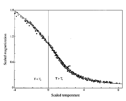
Figure 4: The universal scaling plot of the equation of state of the three-dimensional Heisenberg universality class ($n=3$). The experimental data of five different magnetic materials are shown: $\mathrm{CrBr}_{\scriptscriptstyle 3}$ (characterized by a lattice anisotropy), $\mathrm{EuO}$ (second neighbor interactions), $\mathrm{Ni}$ (itinerant-electron ferromagnet), $\mathrm{YIG}$ (Yttrium Iron Garnet, ferrimagnet), $\mathrm{Pd}_{\scriptscriptstyle 3}\mathrm{Fe}$ (ferromagnetic alloy). Despite of the different interaction details all data collapse onto the universal scaling function. Furthermore the solid line was obtained from a series expansion of the Heisenberg model (see [4, 67]). The figure is taken from H. E. Stanley, Rev. Mod. Phys. 71, S358 (1999).

Second, Figure 4 displays the universal scaling function ${\tilde{M}}(x,1)$ of the three-dimensional Heisenberg universality class. Here the data of five different magnetic materials (note that none of these materials is an idealized ferromagnet [1]) agree with the calculated curve of the Heisenberg model, obtained from a series expansion [67, 4]. Both universal scaling plots demonstrate perfectly the robustness of each universality class with respect to variations of the microscopic interactions.

In addition to the critical exponents and scaling functions one often refers the universality also to certain amplitude combinations (see [68] for an excellent review). These amplitude combinations are very useful in order to identify the universality class of a phase transition since the amplitude combinations vary more widely than the corresponding exponents. Furthermore, the measurement of amplitude combinations in experiments or numerical simulations yields a reliable test for theoretical predictions, obtained e.g. from renormalization group approximations. Consider the singular behavior of the susceptibility by approaching the transition point from above and below

$$\chi(T>T_{\scriptscriptstyle\mathrm{c}},h=0) \sim a_{\scriptscriptstyle\chi,+}\,\delta T^{-\gamma}\,,$$ (1.41)

$$\chi(T<T_{\scriptscriptstyle\mathrm{c}},h=0) \sim a_{\scriptscriptstyle\chi,-}\,(-\delta T)^{-\gamma}\,.$$ (1.42)

The amplitudes $a_{\scriptscriptstyle\chi,+}$ and $a_{\scriptscriptstyle\chi,-}$ are related to the non-universal metric factors and to particular values of universal scaling functions. The universal scaling form of the susceptibility is obtained from Eq. (1.28)

$$\chi(\delta T,h)\;=\;\left(\frac{\partial\,m(\delta T,h)}{\partial\,h}\right)_{T}\;\sim\;a_{\scriptscriptstyle h}\;\lambda^{\gamma}\;\;{\tilde{\mathrm{X}}}(a_{\scriptscriptstyle T}\delta T\,\lambda,a_{\scriptscriptstyle h}h\,\lambda^{\beta\delta})\,,$$ (1.43)

with ${\tilde{\mathrm{X}}}(x,y)=\partial_{\scriptscriptstyle y}{\tilde{M}}(x,y)$. Setting $a_{\scriptscriptstyle T}|\delta T|\lambda=1$ we obtain for the amplitudes

$$a_{\scriptscriptstyle\chi,+} = a_{\scriptscriptstyle h}\,a_{\scriptscriptstyle T}^{-\gamma}\,{\tilde{\mathrm{X}}}(+1,0)\,$$ (1.44)

$$a_{\scriptscriptstyle\chi,-} = a_{\scriptscriptstyle h}\,a_{\scriptscriptstyle T}^{-\gamma}\,{\tilde{\mathrm{X}}}(-1,0)\,.$$ (1.45)

Obviously, the amplitudes $a_{\scriptscriptstyle\chi,+}$ and $a_{\scriptscriptstyle\chi,-}$ are non-universal, but the ratio

$$\frac{a_{\scriptscriptstyle\chi,+}}{\,a_{\scriptscriptstyle\chi,-}\,}\;=\;\frac{\,{\tilde{\mathrm{X}}}(+1,0)\,}{{\tilde{\mathrm{X}}}(-1,0)}$$ (1.46)

is a universal quantity. For example, the mean field behavior of the susceptibility takes the form

$$\chi(\delta T,h=0)\;=\;\frac{1}{\,b_{\scriptscriptstyle 2}\,\delta T\,+\,3\,b_{\scriptscriptstyle 4}\,m^{2}\,}\,,$$ (1.47)

leading to [see Eq. (1.36)]

$$a_{\scriptscriptstyle\chi,+}\,=\,\frac{1}{b_{\scriptscriptstyle 2}}\,,\quad\quad a_{\scriptscriptstyle\chi,-}\,=\,\frac{1}{2\,b_{\scriptscriptstyle 2}}\,,\quad\quad\Longrightarrow\quad\quad\frac{a_{\scriptscriptstyle\chi,+}}{\,a_{\scriptscriptstyle\chi,-}\,}\;=\;2\,.$$ (1.48)

Similar to the amplitude ratio of the susceptibility other universal combinations can be defined. Well known and experimentally important is the quantity (see [68])

$$R_{\chi}\;=\;\Gamma\,D_{\scriptscriptstyle\mathrm{c}}\,B^{\delta-1}\,.$$ (1.49)

Here, $\Gamma$, $D_{\scriptscriptstyle\mathrm{c}}$, $B$ are the traditional, but unfortunately unsystematical, notations for the amplitudes of

$$\left.\chi\sim\Gamma\,\delta T^{-\gamma{\vphantom{\beta}}}\right|_{T>T_{\scriptscriptstyle\mathrm{c}}}\,,\quad\quad\left.h\sim D_{\scriptscriptstyle\mathrm{c}}\,m^{\delta}\right|_{T=T_{\scriptscriptstyle\mathrm{c}}}\,,\quad\quad\left.m\sim B\,(-\delta T)^{\beta}\right|_{T<T_{\scriptscriptstyle\mathrm{c}}}\,.$$ (1.50)

These amplitudes correspond to the values [see Eq. (1.28)]

$$\Gamma=a_{\scriptscriptstyle\chi,+}=a_{\scriptscriptstyle h}\,a_{\scriptscriptstyle T}^{-\gamma}\,{\tilde{\mathrm{X}}}(1,0)\,,\quad\quad D_{\scriptscriptstyle\mathrm{c}}=a_{\scriptscriptstyle h}^{-1}\,{\tilde{M}}(0,1)^{-\delta}\,,\quad\quad B=a_{\scriptscriptstyle T}^{\beta}\,{\tilde{M}}(-1,0)\,.$$ (1.51)

Using the normalizations ${\tilde{M}}(-1,0)={\tilde{M}}(0,1)=1$ we find for the amplitude combination

$$R_{\chi}\;=\;{\tilde{\mathrm{X}}}(1,0)$$ (1.52)

which is obviously a universal quantity. In case of the mean field theory we find $R_{\chi}=1$. These two examples show how the universality of amplitude combinations emerges naturally from the universality of the scaling functions, i.e., universal amplitude combinations are just particular values of the universal scaling functions.

The above presented phenomenological concepts of scaling and universality have been tested in a variety of systems with remarkable success. Nevertheless, they have certain shortcomings. For example, there is no way of determining the critical exponents and scaling functions explicitly. Furthermore, no mathematical substantiation for the underlying scaling form of thermodynamic potentials is provided. It requires Wilson renormalization group theory to remedy these shortcomings. This is sketched in the next section.

1.4 Remarks on renormalization group theory

A foundation for the understanding of the scaling theory and the concept of universality has been provided by Wilson’s renormalization group (RG) theory [15, 16]. In equilibrium systems the RG theory maps the critical point onto a fixed point of a certain transformation of the system’s Hamiltonian (introductions are presented in e.g. [21, 17, 19, 18]). In case of the instructive real space RG [34] the transformation contains a rescaling of a microscopic length scale, e.g. the lattice spacing $a$, by a factor $b$ ($a\mapsto b\,a$) and the elimination of those degrees of freedom that correspond to the range between $a$ and $b\,a$. This rescaling will change the system’s properties away from the critical point where the system exhibits only finite characteristic length scales. But at criticality the infinite correlation length [Eq. (1.5)] determines the physical behavior and the properties of the system remain unaffected by the rescaling procedure. In this way, criticality corresponds to a fixed point of the renormalization transformation.

Denoting the system’s Hamiltonian by ${\mathcal{H}}$ and the rescaled Hamiltonian by ${\mathcal{H}}^{\prime}$ the renormalization transformation is described by an appropriate operator ${\mathcal{R}}$,

$${\mathcal{H}}^{\prime}\;=\;{\mathcal{R}}\circ{\mathcal{H}}\,.$$ (1.53)

Fixed point Hamiltonians ${\mathcal{H}}^{\ast}$ satisfy

$${\mathcal{H}}^{\ast}\;=\;{\mathcal{R}}\circ{\mathcal{H}}^{\ast}\,$$ (1.54)

and it turns out that different fixed point Hamiltonians are related to different universality classes [21]. For the sake of concreteness consider the reduced Ising Hamiltonian

$${\tilde{\mathcal{H}}}\;=\;-\,\frac{\mathcal{H}}{\,k_{\scriptscriptstyle\mathrm{B}}T\,}\;=\;\frac{J}{\,k_{\scriptscriptstyle\mathrm{B}}T\,}\sum_{\scriptscriptstyle\langle i,j\rangle}\,S_{\scriptscriptstyle i}S_{\scriptscriptstyle j}\,+\,\frac{h}{\,k_{\scriptscriptstyle\mathrm{B}}T\,}\sum_{\scriptscriptstyle i}\,S_{\scriptscriptstyle i},$$ (1.55)

with the spin variables $S=\raisebox{0.86108pt}{$\scriptstyle\pm$}1$, the nearest neighbor interaction coupling $J$, and the homogeneous external field $h$, and where the first sum is taken over all pairs of neighboring spins on a given $D$-dimensional lattice. The partition function for a system of $N$ spins is

$$Z_{\scriptscriptstyle N}(K_{\scriptscriptstyle 1},K_{\scriptscriptstyle 2})\;=\;\sum_{\scriptscriptstyle\{S\}}\,{\mathrm{e}}^{{\tilde{\mathcal{H}}}(K_{\scriptscriptstyle 1},K_{\scriptscriptstyle 2})}\,,$$ (1.56)

where the sum is taken over all possible spin configurations and where we introduce the couplings

$$K_{\scriptscriptstyle 1}\;=\;\frac{J}{\,k_{\scriptscriptstyle\mathrm{B}}T\,}\,,\quad\quad K_{\scriptscriptstyle 2}\;=\;\frac{h}{\,k_{\scriptscriptstyle\mathrm{B}}T\,}\,.$$ (1.57)

In general the Hamiltonian can be written as a function of the couplings

$${\tilde{\mathcal{H}}}(\underline{K})\;=\;\sum_{\scriptscriptstyle i}\,K_{\scriptscriptstyle i}\,{\mathcal{O}}_{\scriptscriptstyle i}\,,$$ (1.58)

where ${\mathcal{O}}_{\scriptscriptstyle i}$ are the operators appearing in the Hamiltonian. Performing a renormalization transformation reduces the spin numbers ($N\mapsto N^{\prime}=N/b^{D}$) and leads to a rescaled Hamiltonian, characterized by the couplings

$$K^{\prime}_{\scriptscriptstyle 1}\;=\;K^{\prime}_{\scriptscriptstyle 1}(K_{\scriptscriptstyle 1},K_{\scriptscriptstyle 2})\,,\quad\quad K^{\prime}_{\scriptscriptstyle 2}\;=\;K^{\prime}_{\scriptscriptstyle 2}(K_{\scriptscriptstyle 1},K_{\scriptscriptstyle 2})\,,\quad\quad K^{\prime}_{\scriptscriptstyle 3}\;=\;K^{\prime}_{\scriptscriptstyle 3}(K_{\scriptscriptstyle 1},K_{\scriptscriptstyle 2})\,,\ldots\;.$$ (1.59)

Here, $K^{\prime}_{\scriptscriptstyle i>2}$ account for additional coupling terms of the renormalized Hamiltonian which may appear as a result of the renormalization transformation even if they are not present in the initial Hamiltonian. These so-called RG recursion relations generate trajectories in the space of couplings, i.e., the couplings $\underline{K}$ flow under successive renormalizations

$${\underline{K}}\;\mathop{\longrightarrow}\limits_{\mathcal{R}}\;{\underline{K}}^{\scriptscriptstyle(1)}\;\mathop{\longrightarrow}\limits_{\mathcal{R}}\;{\underline{K}}^{\scriptscriptstyle(2)}\;\mathop{\longrightarrow}\limits_{\mathcal{R}}\;\ldots\;\mathop{\longrightarrow}\limits_{\mathcal{R}}\;{\underline{K}}^{\scriptscriptstyle(n)}\;\mathop{\longrightarrow}\limits_{\mathcal{R}}\;{\underline{K}}^{\scriptscriptstyle(n+1)}\;\mathop{\longrightarrow}\limits_{\mathcal{R}}\;\ldots\,$$ (1.60)

along the RG trajectories towards a certain fixed point ${\underline{K}}^{\ast}$. If the system is not initially at criticality the couplings will flow towards a trivial fixed point, e.g., a fixed points that corresponds to zero or infinite temperature.

Linearizing the problem close to a fixed point yields

$${\mathcal{R}}\circ{\tilde{\mathcal{H}}}({\underline{K}}^{\ast}+\delta{\underline{K}}) = {\tilde{\mathcal{H}}}^{\ast}\,+\,{\mathcal{R}}\circ\sum_{\scriptscriptstyle i}\,\delta K_{\scriptscriptstyle i}\,{\mathcal{O}}_{\scriptscriptstyle i}$$ (1.61)

$$\approx {\tilde{\mathcal{H}}}^{\ast}\,+\,\sum_{\scriptscriptstyle i}\,\delta K_{\scriptscriptstyle i}\,\sum_{\scriptscriptstyle j}{\mathcal{L}}_{\scriptscriptstyle i,j}\,{\mathcal{O}}_{\scriptscriptstyle j}$$

$$= {\tilde{\mathcal{H}}}^{\ast}\,+\,\sum_{\scriptscriptstyle j}\left(\sum_{\scriptscriptstyle i}\,\delta K_{\scriptscriptstyle i}\,{\mathcal{L}}_{\scriptscriptstyle i,j}\right)\,{\mathcal{O}}_{\scriptscriptstyle j}$$

$$= {\tilde{\mathcal{H}}}^{\ast}\,+\,\sum_{\scriptscriptstyle j}\delta K_{\scriptscriptstyle j}^{\prime}\,{\mathcal{O}}_{\scriptscriptstyle j}\,.$$

Assuming that the diagonalized operator ${\mathcal{L}}$ has the eigenoperators $\Omega_{\scriptscriptstyle i}$ and eigenvalues $\Lambda_{\scriptscriptstyle i}$ such that ${\mathcal{L}}\Omega_{\scriptscriptstyle i}=\lambda_{\scriptscriptstyle i}\Omega_{\scriptscriptstyle i}$ we find that the couplings transform in the diagonal representation ($\delta\kappa$) according to $\delta\kappa_{\scriptscriptstyle i}^{\prime}=\Lambda_{\scriptscriptstyle i}\delta\kappa_{\scriptscriptstyle i}$, thus

$${\mathcal{R}}\circ{\tilde{\mathcal{H}}}({\underline{K}}^{\ast}+\delta{\underline{K}})\;=\;{\tilde{\mathcal{H}}}^{\ast}\,+\,\sum_{\scriptscriptstyle i}\,\Lambda_{\scriptscriptstyle i}\,\delta\kappa_{\scriptscriptstyle i}\,{\Omega}_{\scriptscriptstyle i}\,.$$ (1.62)

The couplings $\delta\kappa_{\scriptscriptstyle i}$ are termed scaling fields and their recursion relation can be expressed by the rescaling factor $b$

$$\delta\kappa_{\scriptscriptstyle i}^{\prime}\;=\;b^{y_{\scriptscriptstyle i}}\;\delta\kappa_{\scriptscriptstyle i}\quad\quad{\mathrm{with}}\quad\quad\Lambda_{\scriptscriptstyle i}\;=\;b^{y_{\scriptscriptstyle i}}\,.$$ (1.63)

Successive renormalizations correspond to

$$\delta\kappa_{\scriptscriptstyle i}\;\mathop{\longrightarrow}\limits_{\mathcal{R}}\;b^{y_{\scriptscriptstyle i}}\,\delta\kappa_{\scriptscriptstyle i}\;\mathop{\longrightarrow}\limits_{\mathcal{R}}\;b^{2y_{\scriptscriptstyle i}}\,\delta\kappa_{\scriptscriptstyle i}\;\mathop{\longrightarrow}\limits_{\mathcal{R}}\;b^{3y_{\scriptscriptstyle i}}\,\delta\kappa_{\scriptscriptstyle i}\;\mathop{\longrightarrow}\limits_{\mathcal{R}}\;\ldots\;.$$ (1.64)

Thus, the renormalization flow depends in the vicinity of a given fixed point ${\tilde{\mathcal{H}}}^{\ast}$ on the exponents $y_{\scriptscriptstyle i}$. For $y_{\scriptscriptstyle i}>0$ ($\Lambda_{\scriptscriptstyle i}>1$) the corresponding scaling field $\delta\kappa_{i}$ is called relevant since successive renormalization transformations drive the system away from ${\tilde{\mathcal{H}}}^{\ast}$. In case of a negative exponent $y_{\scriptscriptstyle i}<0$ ($\Lambda_{\scriptscriptstyle i}<1$) the system approaches the fixed point under repeated transformations and the scaling field is termed irrelevant. Marginal scaling fields correspond to $y_{\scriptscriptstyle i}=0$ ($\Lambda_{\scriptscriptstyle i}=1$) and require higher than linear order in the expansion. In this way each fixed point is characterized by its associated scaling fields and by a domain of attraction which corresponds to the set of points flowing eventually to the fixed point. This set forms a hypersurface in the space of couplings and is termed the critical surface.

In summary, a fixed point ${\tilde{\mathcal{H}}}^{\ast}$ is approached if all associated relevant scaling fields are zero, otherwise the system flows away from ${\tilde{\mathcal{H}}}^{\ast}$. Examples for relevant scaling fields in ferromagnetism are the temperature $\delta T$ and the conjugated field $h$. Criticality is only achieved for $\delta T\to 0$ and $h\to 0$, therefore we may identify

$$\delta\kappa_{\scriptscriptstyle 1} = \delta\kappa_{\scriptscriptstyle T}\;=\;a_{\scriptscriptstyle T}\delta T\,,\quad\quad y_{\scriptscriptstyle 1}\;=\;y_{\scriptscriptstyle T}\,>\,0\,,$$ (1.65)

$$\delta\kappa_{\scriptscriptstyle 2} = \delta\kappa_{\scriptscriptstyle h}\;=\;a_{\scriptscriptstyle h}h\,,\;\;\,\quad\quad y_{\scriptscriptstyle 2}\;=\;y_{\scriptscriptstyle h}\,>\,0\,,$$ (1.66)

and $y_{\scriptscriptstyle i>2}<0$. On the other hand, all Hamiltonians that differ from the fixed point ${\tilde{\mathcal{H}}}^{\ast}$ only by irrelevant scaling fields flow towards ${\tilde{\mathcal{H}}}^{\ast}$. For example the five magnetic materials presented in Figure 4 differ only by irrelevant scaling fields.

Although the above linear recursion relations [Eq. (1.63)] describe the RG trajectories only in the vicinities of fixed points they provide some insight in the topology of the entire RG flow (see Figure 5). These RG flow diagrams are useful in order to illustrate the RG transformations schematically and present a classification scheme in terms of fixed point stability. The stability of a given fixed point is determined by the number of relevant and irrelevant scaling fields. Instable fixed points are characterized by at least one relevant scaling field since Hamiltonians arbitrarily close to the fixed point will flow away under successive RG iterations. Ordinary critical points correspond to singly unstable fixed points, i.e., unstable with respect to the control parameter (e.g. temperature) of the phase transition. Tricritical points are characterized by a second instability. An applied external field conjugated to the order parameter implies an additional instability of the fixed point.

Figure 5: Sketch of the renormalization group flow of an Ising ferromagnet (see [Eq. (1.55)]) on a hierarchical lattice. Hierarchical lattices are iteratively constructed lattices [69, 70] where the so-called Migdal-Kadanoff scheme of renormalization is exact [71, 72]. The flowlines show the motion of the coupling constants $x=\exp{(2K_{\scriptscriptstyle 1})}$ (temperature-like variable) and $y=\exp{(K_{\scriptscriptstyle 2})}$ (field-like variable) under successive iterations of the recursion relations $x^{\prime}=(x^{2}+y^{2})(x^{-2}+y^{2})(1+y^{2})^{-2}$ and $y^{\prime}=y^{2}(1+x^{2}y^{2})(x^{2}+y^{2})^{-1}$. The flowlines are attracted and repelled by the fixed points $(1,1)$, $(1,\infty)$, $(\infty,1)$, and $(x_{\scriptscriptstyle c},1)$ with $x_{\scriptscriptstyle c}=3.38298\ldots$. The phase transition corresponds to the non-trivial fixed point $(x_{\scriptscriptstyle c},1)$ with the eigenvalues $\Lambda_{\scriptscriptstyle 1}\approx 1.6785$ and $\Lambda_{\scriptscriptstyle 2}\approx 3.6785$, leading to $\beta\approx 0.16173$ and $\delta\approx 15.549$.

Furthermore, the stability of fixed points depends on the spatial dimensionality $D$ of a system. Above a certain dimension $D_{\scriptscriptstyle\mathrm{c}}$ the scaling behavior is determined by a trivial fixed point with classical mean field exponents, whereas a different fixed point with non-classical exponents determines the scaling behavior below $D_{\scriptscriptstyle\mathrm{c}}$. This exchange of the scaling behavior is caused by an exchange of the stability of the corresponding fixed points below and above $D_{\scriptscriptstyle\mathrm{c}}$ [17, 22, 73]. At the so-called upper critical dimension $D_{\scriptscriptstyle\mathrm{c}}$ both fixed points are identical and marginally stable. The scaling behavior is characterized by mean field exponents modified by logarithmic corrections [74, 20]. We will discuss the scaling behavior of certain non-equilibrium phase transitions at the upper critical dimension in detail in the following chapters.

Let us now consider how scaling emerges from the renormalization transformation. It is essential that the partition function is invariant under the renormalization operation ${\mathcal{R}}$ [21]

$$Z_{\scriptscriptstyle N}(\delta\kappa_{\scriptscriptstyle T},\delta\kappa_{\scriptscriptstyle h},\delta\kappa_{\scriptscriptstyle 3},\ldots)\;=\;Z_{\scriptscriptstyle N^{\prime}}(\delta\kappa^{\prime}_{\scriptscriptstyle T},\delta\kappa_{\scriptscriptstyle h}^{\prime},\delta\kappa_{\scriptscriptstyle 3}^{\prime},\ldots)\,.$$ (1.67)

Therefore, the free energy per degree of freedom transforms according to

$$f(\delta\kappa_{\scriptscriptstyle T},\delta\kappa_{\scriptscriptstyle h},\delta\kappa_{\scriptscriptstyle 3},\ldots)\;=\;b^{-D}\,f(\delta\kappa^{\prime}_{\scriptscriptstyle T},\delta\kappa_{\scriptscriptstyle h}^{\prime},\delta\kappa_{\scriptscriptstyle 3}^{\prime},\ldots)\,.$$ (1.68)

Combining this equation with Eq. (1.63) and using the identifications Eq. (1.65) and Eq. (1.66) yields the scaling form

$$f(a_{\scriptscriptstyle T}\delta T,a_{\scriptscriptstyle h}h,\delta\kappa_{\scriptscriptstyle 3},\ldots)\;\sim\;b^{-D}\,f(b^{y_{\scriptscriptstyle T}}\,a_{\scriptscriptstyle T}\delta T,b^{y_{\scriptscriptstyle h}}\,a_{\scriptscriptstyle h}h,b^{y_{\scriptscriptstyle 3}}\,\delta\kappa_{\scriptscriptstyle 3},\ldots)\,.$$ (1.69)

Introducing $\lambda=b^{y_{\scriptscriptstyle T}}$ we obtain the scaling form of the free energy [see Eq. (1.13)]

$$f(a_{\scriptscriptstyle T}\delta T,a_{\scriptscriptstyle h}h,\delta\kappa_{\scriptscriptstyle 3},\ldots)\;\sim\;\lambda^{\alpha-2}\;\;{f}(a_{\scriptscriptstyle T}\delta T\,\lambda,a_{\scriptscriptstyle h}h\,\lambda^{\beta\delta},\delta\kappa_{\scriptscriptstyle 3}\,\lambda^{\phi_{\scriptscriptstyle 3}},\ldots)\,,$$ (1.70)

where we have identified the exponents

$$y_{\scriptscriptstyle T}\,=\,\frac{1}{\nu}\,,\quad y_{\scriptscriptstyle h}\,=\,\frac{\beta\,\delta}{\nu}\,,\quad y_{\scriptscriptstyle i>2}\,=\,\frac{\phi_{\scriptscriptstyle i>2}}{\nu}\,.$$ (1.71)

The possible additional scaling fields $\delta\kappa_{i>2}$ deserve comments. Irrelevant scaling fields ($\phi_{i>2}<0$) may cause corrections to the asymptotic scaling behavior [75]. For example, choosing $\lambda=1/|a_{\scriptscriptstyle T}\delta T|$ we obtain at zero field

$$f(a_{\scriptscriptstyle T}\delta T,0,\delta\kappa_{\scriptscriptstyle 3}) \sim |a_{\scriptscriptstyle T}\delta T|^{2-\alpha}\;f(\raisebox{0.86108pt}{$\scriptstyle\pm$}1,0,\delta\kappa_{\scriptscriptstyle 3}\,|a_{\scriptscriptstyle T}\delta T|^{|\phi_{\scriptscriptstyle 3}|})$$

$$\approx |a_{\scriptscriptstyle T}\delta T|^{2-\alpha}\,f(\raisebox{0.86108pt}{$\scriptstyle\pm$}1,0,0)+|a_{\scriptscriptstyle T}\delta T|^{2-\alpha+|\phi_{\scriptscriptstyle 3}|}\,\delta\kappa_{\scriptscriptstyle 3}\,\left.\partial_{\scriptscriptstyle x}^{\vphantom{X}}f(\raisebox{0.86108pt}{$\scriptstyle\pm$}1,0,x)\right|_{\scriptscriptstyle x=0}+\ldots\,.$$

The non-universal corrections to the leading order $|\delta T|^{2-\alpha}$ are termed confluent singularities and they determine the size of the critical region. Often confluent singularities have to be taken into account in order to analyze high precision data. Impressive examples of confluent singularity effects of superfluid Helium are reviewed in [55]. The above expansion of $f(\raisebox{0.86108pt}{$\scriptstyle\pm$}1,0,x)$ implies that the free energy is an analytic function in $\delta\kappa_{\scriptscriptstyle 3}$. If the free energy is non-analytic the scaling field $\delta\kappa_{\scriptscriptstyle 3}$ is termed a dangerous irrelevant variable [76, 77]. In that case, the free energy exhibits e.g. a power-law divergence

$$f(x,y,z)\;=\;z^{-\mu}\,{\hat{f}}(x,y)$$ (1.73)

characterized by the exponent $\mu>0$. Singularities of this type occur for example in the mean field regime of the well-known Landau-Ginzburg-Wilson Hamiltonian for short range interacting ferromagnets (see e.g. [78]). There, the dangerous irrelevant variable corresponds to the coupling constant of the $\phi^{4}$ interactions. The nonanalytic behavior leads to the modified scaling form of the free energy

$$f(a_{\scriptscriptstyle T}\delta T,a_{\scriptscriptstyle h}h,\delta\kappa_{\scriptscriptstyle 3}) \sim \lambda^{-\nu D}\;\;{f}(a_{\scriptscriptstyle T}\delta T\,\lambda,a_{\scriptscriptstyle h}h\,\lambda^{\beta\delta},\delta\kappa_{\scriptscriptstyle 3}\,\lambda^{\phi_{\scriptscriptstyle 3}})$$ (1.74)

$$= \left.\lambda^{-\nu D-\mu\phi_{\scriptscriptstyle 3}}\;\delta\kappa_{\scriptscriptstyle 3}^{-\mu}\;{\hat{f}}(a_{\scriptscriptstyle T}\delta T\,\lambda,a_{\scriptscriptstyle h}h\,\lambda^{\beta\delta})\right|_{\scriptscriptstyle h=0}$$

$$= |a_{\scriptscriptstyle T}\delta T|^{\nu D+\mu\phi_{\scriptscriptstyle 3}}\;\delta\kappa_{\scriptscriptstyle 3}^{-\mu}\;{\hat{f}}(\raisebox{0.86108pt}{$\scriptstyle\pm$}1,0)\,.$$

Compared to the standard behavior $f\,{\tilde{\propto}}\,|\delta T|^{2-\alpha}$ the above result reflects the breakdown of the hyperscaling law $2-\alpha=\nu D$. Additionally to the violation of scaling laws, dangerous irrelevant variables also cause the breakdown of common finite-size scaling within the mean field regime [79, 77]. This is well established in equilibrium e.g. in the $n\to\infty$ limit. We will address this point in detail in Chapter 3 where high-dimensional non-equilibrium phase transitions are considered.

The situation is different when the scaling field $\delta\kappa_{\scriptscriptstyle 3}$ is relevant, i.e., $\phi_{\scriptscriptstyle 3}>0$. In that case the free energy at zero field is given by

$$f(a_{\scriptscriptstyle T}\delta T,0,\delta\kappa_{\scriptscriptstyle 3})\;\sim\;|a_{\scriptscriptstyle T}\delta T|^{2-\alpha}\;f(\raisebox{0.86108pt}{$\scriptstyle\pm$}1,0,\delta\kappa_{\scriptscriptstyle 3}\,|a_{\scriptscriptstyle T}\delta T|^{-\phi_{\scriptscriptstyle 3}})\,.$$ (1.75)

For sufficient small arguments ($|\delta\kappa_{\scriptscriptstyle 3}|\delta T|^{-\phi_{\scriptscriptstyle 3}}|\ll 1$) the relevant scaling field leads again to corrections to the asymptotic scaling behavior. But approaching the transition point ($\delta T\to 0$) the scaling argument diverges and gives rise to a different critical behavior, i.e., the system crosses over to a different universality class. We will discuss crossover phenomena in detail in Chapter 5. Eventually a marginal scaling field causes logarithmic corrections via

$$\delta\kappa_{\scriptscriptstyle 3}\,|a_{\scriptscriptstyle T}\delta T|^{-\phi_{\scriptscriptstyle 3}} = \delta\kappa_{\scriptscriptstyle 3}\,\exp{(-\phi_{\scriptscriptstyle 3}\,\ln{|a_{\scriptscriptstyle T}\delta T|})}$$ (1.76)

$$\mathop{\longrightarrow}\limits_{\phi_{\scriptscriptstyle 3}\to 0} \delta\kappa_{\scriptscriptstyle 3}\;(\,1-\phi_{\scriptscriptstyle 3}\,\ln{|a_{\scriptscriptstyle T}\delta T|}\,+\,\ldots)\,.$$

Often, these logarithmic contributions mask the power law singularities and make the analysis of experimental or numerical data notoriously difficult.

Analogous to the free energy, the renormalization group implies the scaling form of the correlation length $\xi$. Performing a renormalization transformation, the correlation length $\xi$, like all length scales, is decreased by the factor $b$,

$$\xi^{\prime}\;=\;b^{-1}\,\xi\,.$$ (1.77)

It is essential for the understanding of phase transitions that fixed points are characterized by an infinite (or trivial zero) correlation length since $\xi$ satisfies at a fixed point

$$\xi^{\prime}=\xi\,.$$ (1.78)

In this way, a singular correlation length, or in other words, scale invariance is the hallmark of criticality. The scaling form of the correlation length is obtained from Eq. (1.77)

$$\xi(\delta\kappa_{\scriptscriptstyle T},\delta\kappa_{\scriptscriptstyle h},\delta\kappa_{\scriptscriptstyle 3},\ldots)\;=\;b\;\xi(\delta\kappa^{\prime}_{\scriptscriptstyle T},\delta\kappa_{\scriptscriptstyle h}^{\prime},\delta\kappa_{\scriptscriptstyle 3}^{\prime},\ldots)\,,$$ (1.79)

yielding with $\lambda=b^{y_{\scriptscriptstyle T}}$ and Eq. (1.63)

$$\xi(a_{\scriptscriptstyle T}\delta T,a_{\scriptscriptstyle h}h,\delta\kappa_{\scriptscriptstyle 3},\ldots)\;\sim\;\lambda^{\nu}\;\;{\xi}(a_{\scriptscriptstyle T}\delta T\,\lambda,a_{\scriptscriptstyle h}h\,\lambda^{\beta\delta},\delta\kappa_{\scriptscriptstyle 3}\,\lambda^{\phi_{\scriptscriptstyle 3}},\ldots)\,.$$ (1.80)

Instead of the real space renormalization considered so far, it is convenient to work in momentum space. This can be achieved by reformulating the above derivations in terms of Fourier transforms. We refer the interested reader to the reviews of [16, 38, 17]. The momentum space formulation allows a perturbative definition of the RG which leads technically to a formulation in terms of Feyman graph expansions. The appropriate small parameter for the perturbation expansion is the dimensionality difference to the upper critical dimension $\epsilon=D_{\scriptscriptstyle\mathrm{c}}-D$ [80], i.e., the $\epsilon$-expansion gives systematic corrections to mean field theory in powers of $\epsilon$. The $\epsilon$-expansion provides a powerful tool for calculating the critical exponents and the scaling functions. For example, the exponent $\gamma$ for $n$-component magnetic systems with short range interactions is given in second order $\epsilon^{2}$ by (see e.g. [73, 81])

$$\gamma\;=\;1\,+\,\epsilon\,\frac{n+2}{2(n+8)}\,+\,\epsilon^{2}\,\frac{(n+2)}{4(n+8)^{3}}\,(n^{2}+22n+52)\,+\,{\mathcal{O}}(\epsilon^{3})\,.$$ (1.81)

Furthermore the Widom-Griffiths scaling function can be written as a power series in $\epsilon$

$${\tilde{H}}(x,1)\;=\;1\,+\,x\,+\,\epsilon\,{\tilde{H}}_{\scriptscriptstyle 1}(x,1)\,+\,\epsilon^{2}\,{\tilde{H}}_{\scriptscriptstyle 2}(x,1)\,+\,{\mathcal{O}}(\epsilon^{3})\,.$$ (1.82)

Obviously the mean field scaling behavior [Eq. (1.39)] is obtained for $\epsilon=0$. The functions become complicated with increasing order and we just note [82]

$${\tilde{H}}_{\scriptscriptstyle 1}(x,1) = \frac{1}{2(n+8)}\;[\,3(x+3)\ln{(x+3)}\,+\,(n-1)(x+1)\ln{(x+1)}$$ (1.83)

$$+\,6\,x\ln{2}\,-\,9(x+1)\ln{3}\,]\,.$$

For ${\tilde{H}}_{\scriptscriptstyle 2}(x,1)$ we refer to the reviews of [73, 81]. Thus the $\epsilon$-expansion provides estimates of almost all quantities of interest as an asymptotic expansion in powers of $\epsilon$ around the mean field values. Unfortunately it is impossible to estimate within this approximation scheme the corresponding error bars since the extrapolation to larger values of $\epsilon$ is uncontrolled. Detailed analyses turn out that the critical exponents are more accurately estimated than the scaling functions and therefore the amplitudes. For example, the $\epsilon^{2}$-approximation [Eq. (1.81)] for the susceptibility exponent of the two-dimensional Ising model ($n=1$, $\epsilon=2$) yields $\gamma\approx 1.642$. This value differs by $6\%$ from the exact value $\gamma=7/4$ [83]. The amplitude ratio of the susceptibility [Eq. (1.46)] can be expanded as [84]

$$\frac{\,{\tilde{\mathrm{X}}}(+1,0)\,}{{\tilde{\mathrm{X}}}(-1,0)}\;=\;2^{\gamma(\epsilon)-1}\;\frac{\gamma(\epsilon)}{\beta(\epsilon)}$$ (1.84)

proposing the estimate $81.14\ldots$ for $\epsilon=2$. This result differs significantly ($115\%$) from the exact value $37.69\ldots$ [83, 85]. The different accuracy reflects a conceptual difference between the universality of critical exponents and the universality of scaling functions. As pointed out clearly in [68], the universality of exponents arises from the linearized RG flow in the vicinity of the fixed point, whereas the scaling functions are obtained from the entire, i.e., non-linear, RG flow. More precisely, the relevant trajectories from the fixed point of interest to other fixed points determine the universal scaling functions. This illuminates also why exponents between different universality classes may differ slightly while the scaling functions and therefore the amplitude combinations differ significantly. Thus deciding on a system’s universality class by considering the scaling functions and amplitude combinations instead of critical exponents appears to be more sensitive. Hence, nothing demonstrates universality more convincing than the universal data-collapse of various systems (as shown in Figure 3 and Figure 4).

Chapter 2 Absorbing phase transitions

The minimization of the free energy is the governing principle of equilibrium statistical physics. In non-equilibrium situations no such framework exists. But nevertheless, the concepts and techniques which were developed for equilibrium critical phenomena can also be applied to non-equilibrium phase transitions. In particular, the order parameter concept, scaling, universality as well as renormalization group analyses are as powerful as in equilibrium, i.e., although they were developed in equilibrium theories their applicability is far beyond. Therefore, numerous non-equilibrium critical phenomena were successfully investigated by such methods, including the geometrical problem of percolation [86, 87, 88], interface motion and depinning phenomena [89, 90, 91], irreversible growth processes like diffusion-limited aggregation [92], as well as turbulence [93, 94]. In the following we focus our attention on a certain class of non-equilibrium phase transitions, the so-called absorbing phase transitions (APT) [95]. These transitions were investigated intensively in the last two decades (see [7, 8] for recent reviews), since they are related to a great variety of non-equilibrium critical phenomena such as forest fires [96, 97], epidemic spreadings in biology [98], catalytic chemical reactions in chemistry [99], spatio-temporal intermittency at the onset of turbulence [100, 101, 102], scattering of elementary particles at high energies and low-momentum transfer [103], interface growth [104], self-organized criticality [105, 106, 107, 108], damage spreading [7, 109, 110], as well as wetting transitions [7, 111]. But like in equilibrium critical phenomena, most of the work focuses onto the determination of the critical exponents, neglecting the determination of the universal scaling functions.

2.1 Definitions and the contact process at first glance

Absorbing phase transitions occur in dynamical systems that are characterized by at least one absorbing state. Any configuration in which a system becomes trapped forever is an absorbing state. The essential physics of absorbing phase transitions is the competition between the proliferation and the annihilation of a quantity of interest $A$, for example particles, energy units, molecules in catalytic reactions, viruses, etc. Often the proliferation and the annihilation processes are described in terms of reaction-diffusion schemes, e.g.,

$${\mathrm{proliferation:}} A\,\longrightarrow\,2\,A\,,\quad 2\,A\,\longrightarrow\,3\,A\,,\quad\hskip 6.45831ptA\,\longrightarrow\,3\,A\,,\ldots$$ (2.1)

$${\mathrm{annihilation:}} A\,\longrightarrow\,0\,,\hskip 8.61108pt\quad 2\,A\,\longrightarrow\,0\,,\hskip 8.61108pt\,\quad 3\,A\,\longrightarrow\,2\,A\,,\ldots\;.$$ (2.2)

Obviously any configuration with zero density ($\rho_{\scriptscriptstyle A}=0$) is an absorbing state if spontaneous particle generation processes

$$0\,\longrightarrow\,A\,,\quad 0\,\longrightarrow\,2\,A\,,\quad 0\,\longrightarrow\,3\,A\,,\ldots$$ (2.3)

do not take place. When the annihilation processes prevail the proliferation processes, the system will eventually reach the absorbing state after a transient regime. On the other hand, the system will be characterized by a non-zero steady-state density $\rho_{\scriptscriptstyle A}$ in the thermodynamic limit if the proliferation processes outweigh the annihilation processes. In the latter case the system is said to be in the active phase whereas the absorbing phase contains all absorbing configurations. Let us assume that the competition between the proliferation and annihilation is described by a single rate $r$. An absorbing phase transition, i.e., a transition from the active phase to the absorbing phase takes place at the critical rate $r_{\scriptscriptstyle\mathrm{c}}$ if the steady state density $\rho_{\scriptscriptstyle A}$ vanishes below $r_{\scriptscriptstyle\mathrm{c}}$

$$\begin{array}[]{rcl}\rho_{\scriptscriptstyle A}=0&{\mathrm{for}}&r<r_{\scriptscriptstyle\mathrm{c}}\,,\\[5.69054pt] \rho_{\scriptscriptstyle A}>0&{\mathrm{for}}&r>r_{\scriptscriptstyle\mathrm{c}}\,.\end{array}$$ (2.4)

In other words, the density $\rho_{\scriptscriptstyle A}$ is the order parameter and the rate $r$ is the control parameter of the absorbing phase transition. Analogous to equilibrium phase transitions, an order parameter exponent $\beta$ can be defined if the order parameter vanishes continuously

$$\rho_{\scriptscriptstyle A}\;\,{\tilde{\propto}}\,\;(r-r_{\scriptscriptstyle\mathrm{c}})^{\beta}\,.$$ (2.5)

It is worth mentioning that absorbing phase transitions have no equilibrium counterparts since they are far from equilibrium per definition. In equilibrium, the associated transition rates between two states satisfy detailed balance [112]. In case of absorbing phase transitions the rate out of an absorbing state is zero. Therefore, an absorbing state can not obey detailed balance with any other active state [95].

For the sake of concreteness, let us consider the so-called contact process (CP) on a $D$-dimensional lattice. The contact process was introduced by Harris [113] in order to model the spreading of epidemics (see for a review [114]). A lattice site may be empty ($n=0$) or occupied ($n=1$) by a particle representing a healthy or an infected site. Infected sites will recover with probability $1-p$ corresponding to a process of particle annihilation. With probability $p$ an infected site will create an offspring at a randomly chosen vacant nearest neighbor site reflecting particle propagation. Thus the dynamics of the contact process is described by the reaction scheme

$$A\longrightarrow\,0\,,\quad\quad\quad A\longrightarrow\,2\,A\,,$$ (2.6)

where the quantity $A$ represents a particle. Particles are considered as active in the sense that they proliferate with rate $p$ and annihilate with rate $1-p$. Empty lattice sites remain inactive and the empty lattice ($\rho(A)=0$) is the unique absorbing state. In the following we denote the density of active sites, i.e., the order parameter of the absorbing phase transition with $\rho_{\scriptscriptstyle\mathrm{a}}$.

In order to provide a deeper insight into absorbing phase transitions, we present a simple but intriguing mean field treatment. The probability that a given lattice is occupied is $\rho_{\scriptscriptstyle\mathrm{a}}$. This particle will be annihilated with probability $1-p$. Thus in an elementary update step the number of particles $n$ is decreased with the probability $p(\Delta n=-1)=\rho_{\scriptscriptstyle\mathrm{a}}(1-p)$. On the other hand, a new particle is created with rate $p$ at a randomly chosen vacant neighbor. The associate probability is $p(\Delta n=1)=\rho_{\scriptscriptstyle\mathrm{a}}\,p(1-\rho_{\scriptscriptstyle\mathrm{a}})$. The number of particles remains unchanged with probability $p(\Delta n=0)=(1-\rho_{\scriptscriptstyle\mathrm{a}})+\rho_{\scriptscriptstyle\mathrm{a}}^{2}p$. Since we have neglected spatial fluctuations and correlations of $\rho_{\scriptscriptstyle\mathrm{a}}$, the above reaction scheme describes the simplest mean field theory of the contact process. This reaction scheme leads to the differential equation

$$\partial_{\scriptscriptstyle t}\rho_{\scriptscriptstyle\mathrm{a}}\;=\;\,p\,\rho_{\scriptscriptstyle\mathrm{a}}(1-\rho_{\scriptscriptstyle\mathrm{a}})\,-\,\rho_{\scriptscriptstyle\mathrm{a}}\,(1-p)\;=\;(2p-1)\rho_{\scriptscriptstyle\mathrm{a}}\,-\,p\,\rho_{\scriptscriptstyle\mathrm{a}}^{2}\,,$$ (2.7)

with the steady state solutions ($\partial_{\scriptscriptstyle t}\rho_{\scriptscriptstyle\mathrm{a}}=0$)

$$\rho_{\scriptscriptstyle\mathrm{a}}\;=\;0\quad\quad\vee\quad\quad\rho_{\scriptscriptstyle\mathrm{a}}\;=\;\frac{2p-1}{p}\quad\mathrm{for}\quad p>0\,.$$ (2.8)

The first equation corresponds to the absorbing state and is unstable for $p>1/2$. The second equation yields unphysical results ($\rho_{\scriptscriptstyle\mathrm{a}}<0$) for $p<1/2$ but describes the order parameter for $p>1/2$. The behavior of the order parameter is sketched in Figure 6. In the vicinity of the critical value $p_{\scriptscriptstyle\mathrm{c}}=1/2$ we find

$$\rho_{\scriptscriptstyle\mathrm{a}}\;=\;2\,\delta p\,+\,{\mathcal{O}}(\delta p^{2})$$ (2.9)

with the reduced control parameter $\delta p=(p-p_{\scriptscriptstyle\mathrm{c}})/p_{\scriptscriptstyle\mathrm{c}}$. Thus the order parameter exponent is $\beta=1$.

Figure 6: Sketch of the steady state behavior (left) of the order parameter of the contact process within the mean field approximation [Eq. (2.8)]. The dashed lines mark unphysical or unstable solutions. The right figure displays the dynamical behavior of the order parameter. The parameters of the presented mean field curves are $\rho_{\scriptscriptstyle{\mathrm{a}},t=0}=1$, $\delta p=0$ and $\delta p=\raisebox{0.86108pt}{$\scriptstyle\pm$}0.02$, respectively.

Consider now the dynamical behavior of the order parameter. Solving Eq. (2.7) we obtain

$$\rho_{\scriptscriptstyle\mathrm{a}}(t)\;=\;\frac{\delta p}{\;p\,+\,({\delta p}/{\rho_{\scriptscriptstyle{\mathrm{a}},t=0}}-p)\;\exp{(-\delta p\;t)}\;}\,.$$ (2.10)

Asymptotically ($t\to\infty$) the order parameter behaves as

$$\left.\rho_{\scriptscriptstyle\mathrm{a}}(t)^{\vphantom{X}}\right|_{\scriptscriptstyle\delta p<0} \sim -\,\delta p\,\left(p-\frac{\delta p}{\rho_{\scriptscriptstyle{\mathrm{a}},t=0}}\right)^{-1}\;{\mathrm{e}}^{\delta p\,t}\,,$$ (2.11)

$$\left.\rho_{\scriptscriptstyle\mathrm{a}}(t)^{\vphantom{X}}\right|_{\scriptscriptstyle\delta p>0} \sim \frac{\,\delta p\,}{p}\;+\;\frac{\delta p}{p^{2}}\left(p-\frac{\delta p}{\rho_{\scriptscriptstyle{\mathrm{a}},t=0}}\right){\mathrm{e}}^{-\delta p\,t}\,.$$ (2.12)

Apart from criticality, the steady state solutions ($\rho_{\scriptscriptstyle\mathrm{a}}=\delta p/p$ and $\rho_{\scriptscriptstyle\mathrm{a}}=0$) are approached exponentially, independent of the initial value $\rho_{\scriptscriptstyle{\mathrm{a}},t=0}$. The associated correlation time diverges as $|\delta p|^{-1}$. At criticality ($\delta p=0$) the order parameter exhibits an algebraic decay

$$\rho_{\scriptscriptstyle\mathrm{a}}(t)\;=\;\frac{1}{\,\rho_{\scriptscriptstyle\rm a,t=0}^{-1}\,+\,p\,t\,}\;\mathop{\longrightarrow}\limits_{t\to\infty}\;\frac{1}{\,p\,t\,}\,.$$ (2.13)

The dynamical behavior of the order parameter is sketched in Figure 6.

Similar to equilibrium phase transitions, it is often possible for absorbing phase transitions to apply an external field that is conjugated to the order parameter. Being a conjugated field it has to destroy the absorbing phase, it has to be independent of the control parameter, and the corresponding linear response function has to diverge at the critical point

$$\chi\;=\;\frac{\partial\,\rho_{\scriptscriptstyle\mathrm{a}}}{\partial\,h}\;\longrightarrow\;\infty\,.$$ (2.14)

For the contact process the conjugated field causes a spontaneous creation of particles ($0\rightarrow A$). Clearly spontaneous particle generation destroys the absorbing state and therefore the absorbing phase transition at all. In the above mean field scheme the conjugated field creates a particle at an empty lattice site with probability $(1-\rho_{\scriptscriptstyle\mathrm{a}})h$. This particle will survive the next update with probability $p$ or will be annihilated with probability $1-p$, respectively. The modified differential equation [Eq. (2.7)] is given by

$$\partial_{\scriptscriptstyle t}\rho_{\scriptscriptstyle\mathrm{a}}\;=\;\delta p\,\rho_{\scriptscriptstyle\mathrm{a}}\,-\,p\,\rho_{\scriptscriptstyle\mathrm{a}}^{2}\,+\,p\,(1-\rho_{\scriptscriptstyle\mathrm{a}})\,h\,.$$ (2.15)

The steady state order parameter is a function of both the control parameter and the conjugated field

$$\rho_{\scriptscriptstyle\mathrm{a}}(\delta p,h)\;=\;\frac{\delta p-p\,h}{2\,p}\,\pm\,\sqrt{\left(\frac{\delta p-p\,h}{2\,p}\right)^{2}\,+\,{h}\;}\,.$$ (2.16)

The solution with the $+$ sign describes the order parameter as a function of the control parameter and of the conjugated field whereas the $-$ sign solution yields unphysical results $\rho_{\scriptscriptstyle\mathrm{a}}<0$. Both solutions are sketched in Figure 7 for various field values. As requested, the absorbing phase is no longer a steady state solution for $h>0$. At criticality ($\delta p=0$) the order parameter behaves as

$$\rho_{\scriptscriptstyle\mathrm{a}}(\delta p=0,h)\;=\;\sqrt{{h}\,}\;+\;{\mathcal{O}}(h)\,.$$ (2.17)

Now we examine the order parameter behavior close to the critical point. Therefore we perform in Eq. (2.15) the limits $\rho_{\scriptscriptstyle\mathrm{a}}\to 0$, $\delta p\to 0$, and $h\to 0$ with the constraints that $\rho_{\scriptscriptstyle\mathrm{a}}/\sqrt{h}$ and $\rho_{\scriptscriptstyle\mathrm{a}}/\delta p$ are finite. The remaining leading order yields

$$\rho_{\scriptscriptstyle\mathrm{a}}(\delta p,h)\;\sim\;\frac{\delta p}{2\,p}\,+\,\sqrt{\left(\frac{\delta p}{2\,p}\right)^{2}\,+\,{h}\;}\,.$$ (2.18)

The Eq. (2.9) and Eq. (2.17) are recovered from this result by setting $h=0$ and $\delta p=0$, respectively. It is straight forward to derive the dynamical behavior of the order parameter $\rho_{\scriptscriptstyle\mathrm{a}}(\delta p,h,t)$ close to the critical point ($\rho_{\scriptscriptstyle\mathrm{a}}\ll 1$). The differential equation Eq. (2.15) yields that the steady state solution is approached from above as

$$\rho_{\scriptscriptstyle\mathrm{a}}(\delta p,h,t)\;\sim\;\frac{\delta p}{2\,p}\,+\,\sqrt{\left(\frac{\delta p}{2\,p}\right)^{2}\,+\,{h}\;}\;\;\left(1\,\raisebox{0.86108pt}{$\scriptstyle\pm$}\,2\,c_{\scriptscriptstyle 0}{\mathrm{e}}^{-t/\xi_{\raisebox{0.0pt}{$\scriptscriptstyle\parallel$}}}\,+\,{\mathcal{O}}({\mathrm{e}}^{-2t/\xi_{\raisebox{0.0pt}{$\scriptscriptstyle\parallel$}}})\,\right)\,,$$ (2.19)

where the constant $c_{\scriptscriptstyle 0}$ contains the initial conditions. The $+$ sign corresponds to initial conditions with $\rho_{\scriptscriptstyle{\mathrm{a}},t=0}>\rho_{\scriptscriptstyle{\mathrm{a}},t\to\infty}$ whereas the $-$ sign is valid for $\rho_{\scriptscriptstyle{\mathrm{a}},t=0}<\rho_{\scriptscriptstyle{\mathrm{a}},t\to\infty}$. Again, the steady state value is exponentially approached independent of the initial condition. The corresponding temporal correlation length is usually denoted as $\xi_{\raisebox{0.0pt}{$\scriptscriptstyle\parallel$}}$ for absorbing phase transitions, and we find [115]

$$\xi_{\raisebox{0.0pt}{$\scriptscriptstyle\parallel$}}(\delta p,h)\;=\;\frac{1}{2\,p\,\sqrt{\left(\frac{\delta p}{2p}\right)^{2}+h\,}\,}\,.$$ (2.20)

Thus the correlation time diverges at the critical point as

$$\xi_{\raisebox{0.0pt}{$\scriptscriptstyle\parallel$}}(\delta p,h=0)\;=\;|\delta p|^{-1}\quad\quad{\mathrm{and}}\quad\quad\xi_{\raisebox{0.0pt}{$\scriptscriptstyle\parallel$}}(\delta p=0,h)\;=\;\frac{1}{2\,p}\,h^{-1/2}\,.$$ (2.21)

The zero-field singularity is usually associated with the temporal correlation length exponent $\nu_{\raisebox{0.0pt}{$\scriptscriptstyle\parallel$}}=1$.

Furthermore, the derivative of $\rho_{\scriptscriptstyle\mathrm{a}}$ with respect to the conjugated field yields the order parameter susceptibility

$$\chi(\delta p,h)\;=\;\frac{\partial\,\rho_{\scriptscriptstyle\mathrm{a}}}{\partial\,h}\;\sim\;\frac{1}{2}\;\left[\left(\frac{\delta p}{2\,p}\right)^{2}\,+\,{h}\;\right]^{\,-1/2}\,.$$ (2.22)

As required, the order parameter susceptibility becomes infinite at the transition point

$$\left.\chi(\delta p,h)^{\vphantom{X}}\right|_{h\to 0\,} \propto |\delta p|^{-1}\;\;\,\mathop{\longrightarrow}\limits_{\delta p\to 0}\;\infty\,,$$ (2.23)

$$\left.\chi(\delta p,h)^{\vphantom{X}}\right|_{\delta p\to 0} \propto h^{-1/2}\;\;\;\mathop{\longrightarrow}\limits_{h\to 0}\;\infty\,.$$ (2.24)

The mean field behavior of the susceptibility is displayed in Figure 7.

Figure 7: The mean field order parameter (left) and the mean field order parameter susceptibility (right) of the contact process. The dashed lines mark unphysical or unstable solutions. Thick lines correspond to the zero-field behavior whereas the thin lines sketch the smooth non-zero field behavior. The susceptibility displays a finite peak for non-zero field. In the limit $h\to 0$ this peak diverges signalling the critical point.

It is possible to incorporate spatial variations of the order parameter in the mean field theory. Therefore Eq. (2.15) has to be modified and we assume that the order parameter obeys close to criticality ($\rho_{\scriptscriptstyle\mathrm{a}}\ll 1$)

$$\partial_{\scriptscriptstyle t}\rho_{\scriptscriptstyle\mathrm{a}}(\underline{x},t)\;=\;\delta p\,\rho_{\scriptscriptstyle\mathrm{a}}(\underline{x},t)\,-\,p\,\rho_{\scriptscriptstyle\mathrm{a}}(\underline{x},t)^{2}\,+\,p\,h\,+\,\Gamma\,\nabla^{2}\rho_{\scriptscriptstyle\mathrm{a}}(\underline{x},t)\,,$$ (2.25)

where $\rho_{\scriptscriptstyle\mathrm{a}}(\underline{x},t)$ represents the local particle density and where we add the diffusive coupling with $\Gamma>0$. Usually, continuous equations like Eq. (2.25) are obtained from microscopic models by a coarse graining procedure or they are phenomenologically motivated by a Landau expansion [30]. According to Landau, a given system is described by an appropriate functional containing all analytic terms that are consistent with the symmetries of the microscopic problem. Consider small spatial deviations from the homogeneous steady state value $\rho_{\scriptscriptstyle\mathrm{a}}(\delta p,h)$ [Eq. (2.18)] by introducing $\delta\rho_{\scriptscriptstyle\mathrm{a}}(\underline{x},t)=\rho_{\scriptscriptstyle\mathrm{a}}(\underline{x},t)-\rho_{\scriptscriptstyle\mathrm{a}}(\delta p,h)$. The order parameter variations $\delta\rho_{\scriptscriptstyle\mathrm{a}}(\underline{x},t)$ obey the differential equation

$$\partial_{\scriptscriptstyle t}\,\delta\rho_{\scriptscriptstyle\mathrm{a}}(\underline{x},t)\;=\;[\delta p\,-\,2\,p\,\rho_{\scriptscriptstyle\mathrm{a}}(\delta p,h)]\;\delta\rho_{\scriptscriptstyle\mathrm{a}}(\underline{x},t)\,+\,\Gamma\,\nabla^{2}\,\delta\rho_{\scriptscriptstyle\mathrm{a}}(\underline{x},t)\,+\,{\mathcal{O}}(\delta\rho_{\scriptscriptstyle\mathrm{a}}^{2})\,,$$ (2.26)

where nonlinear terms are neglected. Working in Fourier space and using Eq. (2.18) we find that small deviations with wavevector $\underline{k}$ decay as

$$\partial_{\scriptscriptstyle t}\,\delta\rho_{\scriptscriptstyle\mathrm{a}}(\underline{k},t)\;=\;-\,\Gamma\,\left[k^{2}\,+\,\xi_{\raisebox{0.0pt}{$\scriptscriptstyle\perp$}}^{-2}\,\right]\;\delta\rho_{\scriptscriptstyle\mathrm{a}}(\underline{k},t)\,.$$ (2.27)

Here, the characteristic length

$$\xi_{\raisebox{0.0pt}{$\scriptscriptstyle\perp$}}(\delta p,h)\;=\;\sqrt{\,\frac{\Gamma}{2\,p}\,}\;\left[\left(\frac{\delta p}{2\,p}\right)^{2}\,+\,{h}\;\right]^{\,-1/4}$$ (2.28)

is introduced that describes spatial correlations of the order parameter variations [116, 117]. Approaching the transition point, the spatial correlation length becomes infinite

$$\xi_{\raisebox{0.0pt}{$\scriptscriptstyle\perp$}}(\delta p,h=0)\;=\;\sqrt{\Gamma\,}\,|\delta p|^{-1/2}\quad\quad{\mathrm{and}}\quad\quad\xi_{\raisebox{0.0pt}{$\scriptscriptstyle\perp$}}(\delta p=0,h)\;=\;\sqrt{\frac{\Gamma}{2\,p}\,}\,h^{-1/4}\,.$$ (2.29)

Thus the mean field value of the exponent of the correlation length at zero field is $\nu_{\raisebox{0.0pt}{$\scriptscriptstyle\perp$}}=1/2$. Note that the temporal and spatial correlation length are related via [115]

$$\xi_{\raisebox{0.0pt}{$\scriptscriptstyle\perp$}}^{2}\;=\;\Gamma\,\xi_{\raisebox{0.0pt}{$\scriptscriptstyle\parallel$}}\,.$$ (2.30)

Solving Eq. (2.27) and taking the inverse transform we obtain the order parameter variations

$$\delta\rho_{\scriptscriptstyle\mathrm{a}}(\underline{x},t)\;=\;\rho_{\scriptscriptstyle{\mathrm{a}},0}\,\left(\frac{1}{4\,\pi\,\Gamma\,t}\,\right)^{D/2}\;{\mathrm{e}}^{-t/\xi_{\raisebox{0.0pt}{$\scriptscriptstyle\parallel$}}}\;{\mathrm{e}}^{-(\underline{x}-{\underline{x}}_{\scriptscriptstyle 0})^{2}/4\Gamma t}\,,$$ (2.31)

where we have assumed a seed-like initial density variation $\delta\rho_{\scriptscriptstyle\mathrm{a}}(\underline{x},t=0)=\rho_{\scriptscriptstyle{\mathrm{a}},0}\delta(\underline{x}-{\underline{x}}_{\scriptscriptstyle 0})$. Similar to the homogeneous case the lifetime of the localized density fluctuation is determined by the temporal correlation time $\xi_{\raisebox{0.0pt}{$\scriptscriptstyle\parallel$}}$. Furthermore the activity diffuses over regions of distance $\sqrt{2\Gamma t\,}$ from the origin ${\underline{x}}_{\scriptscriptstyle 0}$.

Fluctuations within the steady state can be investigated by adding an appropriate noise term $\eta({\underline{x}},t)$ in Eq. (2.25) representing rapidly-varying degrees of freedom (see e.g. [115, 116]). The noise has zero mean and the correlator is assumed to be given by

$$\langle\,\eta({\underline{x}},t)\,\eta({\underline{x}}^{\prime},t^{\prime})\,\rangle\;=\;\kappa\;\rho_{\scriptscriptstyle\mathrm{a}}\;\delta({\underline{x}}-{\underline{x}}^{\prime})\;\delta(t-t^{\prime})\,.$$ (2.32)

In that case, the mean field steady state fluctuations are given by [116]

$$\langle\,\delta\rho_{\scriptscriptstyle\mathrm{a}}^{2}\,\rangle\;\propto\;\frac{\kappa}{\,4p\,}\;\frac{\,\frac{\delta p}{2\,p}\,+\,\sqrt{\left(\frac{\delta p}{2\,p}\right)^{2}\,+\,{h}\;}\,}{\sqrt{\left(\frac{\delta p}{2\,p}\right)^{2}\,+\,{h}\;}\,}\,.$$ (2.33)

For zero-field the fluctuations reduce to

$$\langle\,\delta\rho_{\scriptscriptstyle\mathrm{a}}^{2}\rangle\,\ \;\propto\;\left\{\begin{array}[]{ll}0&\mathrm{if}\quad\delta p<0\\[5.69054pt] \kappa/2p&\mathrm{if}\quad\delta p>0\,,\end{array}\right.$$ (2.34)

i.e., the fluctuations do not diverge at the critical point but exhibit a finite jump.

In summary, the mean field theory presented above describes the absorbing phase transition of the contact process. The steady state and dynamical order parameter behavior have been derived and certain critical exponents are determined. In contrast to the one characteristic length scale of ordinary critical equilibrium systems, absorbing phase transitions are characterized by two length scales, $\xi_{\raisebox{0.0pt}{$\scriptscriptstyle\perp$}}$ and $\xi_{\raisebox{0.0pt}{$\scriptscriptstyle\parallel$}}$, with different critical exponents $\nu_{\raisebox{0.0pt}{$\scriptscriptstyle\perp$}}$ and $\nu_{\raisebox{0.0pt}{$\scriptscriptstyle\parallel$}}$. This scaling behavior of directed percolation can be interpreted in terms of so-called strongly anisotropic scaling [118], where a different steady state scaling behavior occurs along different directions (indicated by different critical exponents, $\nu_{\raisebox{0.0pt}{$\scriptscriptstyle\parallel$}}/\nu_{\raisebox{0.0pt}{$\scriptscriptstyle\perp$}}\neq 1$). Paradigms of strongly anisotropic scaling are Lifshitz points [119], e.g. in Ising models with competing interactions [120, 121].

Unfortunately, the notations of some critical exponents for absorbing phase transitions differ from those of equilibrium systems. In particular the field dependence of the order parameter at the critical isotherm is written as [7]

$$\rho_{\scriptscriptstyle\mathrm{a}}(\delta p=0,h)\;\,{\tilde{\propto}}\,\;h^{\beta/\sigma}\,,$$ (2.35)

in contrast to the usual equilibrium notation $M\,{\tilde{\propto}}\,h^{1/\delta}$. Thus the field exponent $\sigma$ corresponds in equilibrium to $\beta\,\delta$, i.e., the exponent $\sigma$ of absorbing phase transitions is identical to the gap exponent $\Delta=\beta\,\delta$ of equilibrium systems. In order to avoid friction with the literature of absorbing phase transitions, where $\delta$ is reserved to describe the dynamical scaling behavior, we will use the notation of Eq. (2.35) in the following. Eventually we summarize that the mean field theory is characterized by the exponents $\beta=1$, $\sigma=2$, $\nu_{\raisebox{0.0pt}{$\scriptscriptstyle\parallel$}}=1$, $\nu_{\raisebox{0.0pt}{$\scriptscriptstyle\perp$}}=1/2$, as well as $\gamma=1$, where the latter one describes the divergence of the zero-field susceptibility ($\chi\,{\tilde{\propto}}\,|\delta p|^{-\gamma}$).

2.2 Numerical simulation methods

Despite the simplicity of the contact process, a rigorous solution is still lacking. Like in equilibrium the mean field theory provides correct results only above the upper critical dimension $D_{\scriptscriptstyle\mathrm{c}}$. It fails below $D_{\scriptscriptstyle\mathrm{c}}$ since different sites are strongly correlated whereas they are considered as independent within the mean field approach. Beside of approximation schemes like series expansions [122, 123, 124, 125, 126, 127, 128, 129, 130, 131, 132, 133] and $\epsilon$-expansion within renormalization group approaches, numerical simulations were intensively used in order to determine the critical behavior of the contact process and related models. There are two primary ways to perform numerical simulations of lattice models exhibiting absorbing phase transitions. The first method is to study the steady state behavior of certain quantities of interest, e.g., the order parameter and its fluctuations as a function of various parameters like the control parameter and the external field (e.g. [134, 135, 136, 137]). Especially the equation of state as well as the susceptibility can be obtained in that way [138, 139, 140, 141, 142, 143]. But approaching the critical point, the simulations are affected by diverging fluctuations and correlations causing finite-size and critical slowing down effects (see e.g. [112]). Techniques such as finite-size scaling analysis have to be applied in order to handle these effects.

In contrast to steady state measurements, the second method is based on the dynamical scaling behavior. Often the evolution of a prepared state close to the absorbing phase is investigated. For example the spreading of activity started from a single seed is studied in the vicinity of the critical point [144]. This method is known to be very efficient and the critical exponents can be determined with high accuracy (see for instance [24, 145, 146, 147, 148, 149, 150, 151]). A drawback of this technique is that it is restricted to the vicinity of the absorbing state. For example the conjugated field drives the systems away from the absorbing phase and can therefore not be incorporated. In the following both methods are discussed and the associated exponents are defined. For the sake of concreteness corresponding data of the five-dimensional contact process are presented as an exemplification and are compared to the mean field results.

2.2.1 Steady state scaling behavior

Figure 8: The density of active sites $\rho_{\scriptscriptstyle\mathrm{a}}$ as a function of time for the five-dimensional contact process ($L=16$, $\delta p=0.02$, and $\rho_{\scriptscriptstyle{\mathrm{a}},t=0}=1$). After a transient regime, which depends on the initial configuration, the density of active sites fluctuates around the steady state value $\rho_{\scriptscriptstyle\mathrm{a}}$ (dashed line).

In order to perform simulations of a system exhibiting an absorbing phase transition we have to specify the lattice type and the boundary conditions. In case of the contact process it is customary to consider $D$-dimensional simple cubic lattices of linear size $L$ and periodic boundary conditions. Steady state simulations usually start far away from the absorbing state, e.g. with a fully occupied lattice. The system is updated according to the microscopic rules presented on page 2.6 using a randomly sequential update scheme. Therefore all occupied sites are listed and one active site after the other is updated, selected at random. After a sufficient number of update steps the system reaches a steady state where the number of active sites fluctuates around the average value (see Figure 8). It is customary to interpret one complete lattice update with $n_{\scriptscriptstyle\mathrm{a}}$ active sites as one time step ($t\to t+1$). Thus an elementary update of one lattice site corresponds to a time increment $t\to t+1/n_{\scriptscriptstyle\mathrm{a}}$. Monitoring the density of active sites $\rho_{\scriptscriptstyle\mathrm{a}}(t)$ in the steady state one obtains an estimate of the order parameter $\rho_{\scriptscriptstyle\mathrm{a}}=\langle\rho_{\scriptscriptstyle\mathrm{a}}(t)\rangle$ as well as of its fluctuations

$$\Delta\rho_{\scriptscriptstyle\mathrm{a}}\;=\;L^{D}\,\left(\,\langle\rho_{\scriptscriptstyle\mathrm{a}}(t)^{2}\rangle\,-\,\langle\rho_{\scriptscriptstyle\mathrm{a}}(t)\rangle^{2}\,\right)\,,$$ (2.36)

where $\langle\ldots\rangle$ corresponds to the temporal average

$$\langle\rho_{\scriptscriptstyle\mathrm{a}}(t)^{k}\rangle\;=\;\frac{1}{T}\,\sum_{\scriptscriptstyle t=1}^{\scriptscriptstyle T}\,\rho_{\scriptscriptstyle\mathrm{a}}(t)^{k}\,.$$ (2.37)

Of course reliable results are only obtained if the number of update steps significantly exceeds the correlation time $T\gg\xi_{\raisebox{0.0pt}{$\scriptscriptstyle\parallel$}}$. This becomes notoriously difficult close to the critical point since $\xi_{\raisebox{0.0pt}{$\scriptscriptstyle\parallel$}}\to\infty$. Furthermore the accuracy can be improved if an additional averaging over different initial configurations is performed.

The average density of active sites as well as its fluctuations are plotted in Figure 9 as a function of the control parameter $p$ for various system sizes $L$. As can be seen the order parameter tends to zero in the vicinity of $p\approx 0.532$. Assuming that the scaling behavior of $\rho_{\scriptscriptstyle\mathrm{a}}$ obeys asymptotically the power law

$$\rho_{\scriptscriptstyle\mathrm{a}}(p)\;\,{\tilde{\propto}}\,\;(p-p_{\scriptscriptstyle\mathrm{c}})^{\beta}\,,$$ (2.38)

the critical value $p_{\scriptscriptstyle\mathrm{c}}$ is varied until a straight line in a log-log plot is obtained (see Figure 9). Convincing results are observed for $p_{\scriptscriptstyle\mathrm{c}}=0.53237\raisebox{0.86108pt}{$\scriptstyle\pm$}0.00006$ and the corresponding curve is shown in Figure 9. For $p_{\scriptscriptstyle\mathrm{c}}=0.53231$ and $p_{\scriptscriptstyle\mathrm{c}}=0.53243$ significant curvatures in the log-log plot occur. In this way it is possible to estimate the critical value $p_{\scriptscriptstyle\mathrm{c}}$ as well as its error-bars. Then a regression analysis yields the value of the order parameter exponent $\beta=0.991\raisebox{0.86108pt}{$\scriptstyle\pm$}0.015$ in agreement with the mean field value $\beta=1$.

Figure 9: The order parameter (upper left) and its fluctuations (upper right) of the five-dimensional contact process for various system sizes $L$. The data are averaged over at least $T=10^{7}$ lattice updates. The lower figures show the order parameter as a function of $p-p_{\scriptscriptstyle\mathrm{c}}$. The dashed line corresponds to the mean field behavior with $\beta=1$. A straight line is obtained for $p_{\scriptscriptstyle\mathrm{c}}=0.53237$, whereas $p_{\scriptscriptstyle\mathrm{c}}=0.53243$ and $p_{\scriptscriptstyle\mathrm{c}}=0.53231$ lead to significant curvatures (see lower right figure). For the sake of simplicity lines are plotted instead of symbols.

Usually the order parameter fluctuations diverge at the transition point

$$\Delta\rho_{\scriptscriptstyle\mathrm{a}}\;\,{\tilde{\propto}}\,\;(p-p_{\scriptscriptstyle\mathrm{c}})^{-\gamma^{\prime}}\,.$$ (2.39)

But as can be seen the fluctuations are characterized by a finite jump at $p_{\scriptscriptstyle\mathrm{c}}$ corresponding to the value $\gamma^{\prime}=0$. This agrees well with the mean field result Eq. (2.34). We will see in the next chapter that low-dimensional systems are characterized by a non-zero exponent.

The effects of finite system sizes deserve comment. Of course a finite system reaches the absorbing state with a finite probability even for $p>p_{\scriptscriptstyle\mathrm{c}}$. But this probability tends to zero for $L\to\infty$. It turns out that sufficiently large systems will never reach the absorbing phase within reasonable simulation times for $p>p_{\scriptscriptstyle\mathrm{c}}$. The situation changes close to the transition point since the finite system size $L$ prevents the correlation length $\xi_{\raisebox{0.0pt}{$\scriptscriptstyle\perp$}}$ from becoming infinite. As a result so-called finite-size effects occur, i.e., the corresponding singularities become rounded and shifted (see for example [112]). A typical feature of finite-size effects in equilibrium systems is that a given system may pass within the simulations from one phase to the other. This behavior is caused by critical fluctuations that increases if one approaches the transition point. In case of absorbing phase transitions the scenario is different. Approaching the transition point the correlation length $\xi_{\raisebox{0.0pt}{$\scriptscriptstyle\perp$}}$ increases and as soon as $\xi_{\raisebox{0.0pt}{$\scriptscriptstyle\perp$}}$ is of the order of $L$ the system may pass to an absorbing state and is trapped forever. For example finite-size effects are expected to occur for $\delta p<\Gamma L^{-2}$ according to the mean field result Eq. (2.29). In that case the absorbing state is reached by finite fluctuations even for $p>p_{\scriptscriptstyle\mathrm{c}}$. A simple way to handle that problem is to increase the system size before finite-size effects occur (see Figure 9). Considering overlapping data regions for different system sizes ensures that the obtained results are not affected by finite-size effects. Additionally it is suggested (see, for instance [135]) to consider metastable or quasisteady-state values of the order parameter. But as pointed out in [152] this method is inefficient and can be seriously questioned since the metastable values are not well defined.

Figure 10: The order parameter (upper left) and its fluctuations (upper right) of the five-dimensional contact process for various field values ($h=3\,10^{-5},8\,10^{-6},10^{-6}$). The order parameter and the fluctuations exhibit an analytic behavior for non-zero field. The order parameter susceptibility (lower left) displays the characteristic peak at the critical point (dashed line). The lower right figure shows the order parameter as a function of the conjugated field at $p=p_{\scriptscriptstyle\mathrm{c}}$ for various system sizes $L=4,8,16$ (from right to left). The dashed line corresponds to the mean field behavior with $\beta/\sigma=1/2$.

A better way to analyze finite-size effects for absorbing phase transitions is to incorporate the conjugated field. Due to the conjugated field the system cannot be trapped forever in the absorbing phase. Therefore steady state quantities are available for all values of the control parameter. Analogous to equilibrium phase transitions, the conjugated field results in a rounding of the zero-field curves, i.e., the order parameter and its fluctuations behave smoothly as a function of the control parameter $p$ for finite field values (see Figure 10). For $h\to 0$ we recover the non-analytical behavior of $\rho_{\scriptscriptstyle\mathrm{a}}$ and $\Delta\rho_{\scriptscriptstyle\mathrm{a}}$, respectively. Furthermore, the order parameter susceptibility $\chi$ can be obtained by performing the numerical derivative of the order parameter $\rho_{\scriptscriptstyle\mathrm{a}}(\delta p,h)$ with respect to the conjugated field [Eq. (2.14)]. Similar to the mean field solution the susceptibility displays the characteristic peak at the critical point $p_{\scriptscriptstyle\mathrm{c}}$. In the limit $h\to 0$ this peak diverges, signalling the critical point.

The order parameter and fluctuation data presented in Figure 10 are obtained from simulations where the correlation length is small compared to the systems size. Thus these data do not suffer from finite-size effects. But approaching the transition point finite-size effects emerge. Figure 10 shows the order parameter at $p_{\scriptscriptstyle\mathrm{c}}$ as a function of the conjugated field. The behavior of the infinite system ($L\gg\xi_{\raisebox{0.0pt}{$\scriptscriptstyle\perp$}}$) agrees with the mean field result $\rho_{\scriptscriptstyle\mathrm{a}}\,{\tilde{\propto}}\,h^{1/2}$. Approaching the transition point ($h\to 0$), finite-size effects, i.e., deviations from the behavior of the infinite system occur. The larger the system size $L$ the larger is the scaling regime where the power-law behavior is observed. In this way it is possible to study finite-size effects of steady state measurements in absorbing phase transitions. A detailed analysis of the order parameter, the fluctuations, as well as of a fourth order cumulant is presented in the next chapter. Similar to equilibrium phase transitions, we formulate scaling forms which incorporate the system size as an additional scaling field.

2.2.2 Dynamical scaling behavior

Figure 11: The dynamical behavior of the order parameter of the five-dimensional contact process for $L=32$. The parameters of the presented curves are $\delta p=0$, $\delta p=\raisebox{0.86108pt}{$\scriptstyle\pm$}0.02$ (thick lines), $\delta p=\raisebox{0.86108pt}{$\scriptstyle\pm$}0.00006$ (thin lines) respectively. The data are averaged over at least $N=10^{3}$ different runs. Started from a fully occupied lattice ($\rho_{\scriptscriptstyle{\mathrm{a}},t=0}=1$) the order parameter saturates for $p>p_{\scriptscriptstyle\mathrm{c}}$ and decays exponentially for $p<p_{\scriptscriptstyle\mathrm{c}}$. At the critical point the order parameter displays an algebraic decay. The dashed line corresponds to the mean field exponent $\alpha=1$ and is shown to guide the eye.

In the following we investigate the dynamical scaling behavior at zero field close to the critical point. First, we consider how the order parameter decays starting from a fully occupied lattice, i.e., starting from a so-called homogenous particle source. Studying the temporal evolution of the system one has to average over different runs $\rho_{\scriptscriptstyle\mathrm{a}}(t)=[\rho_{\scriptscriptstyle\mathrm{a}}(t,n_{\scriptscriptstyle{\mathrm{rnd}}})]$ with

$$[\rho_{\scriptscriptstyle\mathrm{a}}(t)]\;=\;\frac{1}{N}\,\sum_{\scriptscriptstyle k=1}^{\scriptscriptstyle N}\,\rho_{\scriptscriptstyle\mathrm{a}}(t,n_{\scriptscriptstyle{\mathrm{rnd}},k})\,.$$ (2.40)

Here, $n_{\scriptscriptstyle{\mathrm{rnd}}}$ denotes the seed number of the random number generator. Simulation results for various values of the control parameter are shown in Figure 11.

Similar to the mean field behavior [Eqs. (2.11-2.13)], the order parameter tends exponentially to the steady state value above $p_{\scriptscriptstyle\mathrm{c}}$ (positive curvature in the log-log plot). Below the transition point the absorbing state is approached exponentially (negative curvature). At the critical point the order parameter decays asymptotically as

$$\rho_{\scriptscriptstyle\mathrm{a}}(t)\;\,{\tilde{\propto}}\,\;t^{-\alpha}\,.$$ (2.41)

As can be seen in Figure 11 the decay exponent agrees with the mean field value $\alpha=1$. Again, deviations from the power-law behavior allow to estimate the critical value $p_{\scriptscriptstyle\mathrm{c}}$. The obtained result and its uncertainty is in agreement with the steady state measurement $p_{\scriptscriptstyle\mathrm{c}}=0.53237\pm 0.00006$.

More accurate estimates for the critical value $p_{\scriptscriptstyle\mathrm{c}}$ and for the critical exponents can be obtained by considering the activity spreading generated from a single active seed [144], a so-called localized particle source. Three typical snapshots of activity spreading of the one-dimensional contact process are shown in Figure 12. Below the critical point the activity ceases after a certain transient regime whereas above $p_{\scriptscriptstyle\mathrm{c}}$ the activity spreading continues infinitely with a finite probability. At the transition point a cluster is generated by the temporal evolution that exhibits fractal properties [145]. Interpreting active sites, e.g., as viruses this figure illustrates the spreading of epidemics through a population.

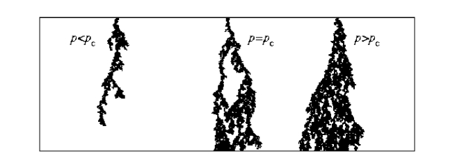
Figure 12: Snapshots of activity spreading in the one-dimensional contact process (time increases downward from $t=0$ to $10^{3}$). The parameters of the presented clusters are $\delta p=0$ and $\delta p=\raisebox{0.86108pt}{$\scriptstyle\pm$}0.02$.

In order to analyze the scaling behavior of activity spreading it is useful to measure the survival probability $P_{\scriptscriptstyle\mathrm{a}}(t)$, the number of active sites $N_{\scriptscriptstyle\mathrm{a}}(t)$ as well as the average mean square distance of the spreading $R_{\scriptscriptstyle\mathrm{a}}(t)^{2}$ [144]. Here, $N_{\scriptscriptstyle\mathrm{a}}(t)$ is averaged over all clusters whereas $R_{\scriptscriptstyle\mathrm{a}}(t)^{2}$ is averaged only over surviving clusters. At criticality, the following power-law behavior are expected to occur asymptotically

$$P_{\scriptscriptstyle\mathrm{a}}(t)\,\,{\tilde{\propto}}\,\,t^{-\delta}\,,\quad\quad N_{\scriptscriptstyle\mathrm{a}}(t)\,\,{\tilde{\propto}}\,\,t^{\theta}\,,\quad\quad R_{\scriptscriptstyle\mathrm{a}}(t)^{2}\,\,{\tilde{\propto}}\,\,t^{2/z}\,,$$ (2.42)

where we have used the notation of [7]. The so-called dynamical exponent $z$ describes the relationship between spatial and temporal correlations and is therefore identified as

$$z\;=\;\frac{\,\nu_{\raisebox{0.0pt}{$\scriptscriptstyle\parallel$}}\,}{\nu_{\raisebox{0.0pt}{$\scriptscriptstyle\perp$}}}\,.$$ (2.43)

According to Eq. (2.30) the mean field value is given by $z=2$. The survival probability $P_{\scriptscriptstyle\mathrm{a}}(t)$ is shown in Figure 13. Again, a positive curvature for $t\to\infty$ indicates in a log-log plot the active phase whereas a negative curvature indicates the absorbing phase. Similar to the steady state [Eq. (2.38)] and dynamical [Eq. (2.41)] order parameter behavior, the survival probability obeys power-law behavior Eq. (2.42) only asymptotically, i.e., confluent singularities have to be taken into consideration. Often, local slopes are considered

$$\delta_{\scriptscriptstyle{\mathrm{local}}}(t)\,=\,-\,\frac{\,\ln{[\,P_{\scriptscriptstyle\mathrm{a}}(t)\,/\,P_{\scriptscriptstyle\mathrm{a}}(t/c)\,]}\,}{\ln{c}}$$ (2.44)

to handle this problem. The parameter $c$ defines the distance of the local slopes and typical values used in previous studies are for example $c=4$ [153], $c=5$ [149, 154], $c=8$ [145] as well as $c=10$ [155]. Of course, for $c\to 1$ the local slopes equals the so-called effective exponent [156]

$$\delta_{\scriptscriptstyle\mathrm{eff}}(t)\;=\;-\,\frac{\partial\,\ln{P_{\scriptscriptstyle\mathrm{a}}(t)}}{\partial\,\ln{t}}\,.$$ (2.45)

The analysis of the local slope is illustrated in Figure 13. Above criticality the local slope tends to zero whereas $\delta_{\mathrm{local}}(t)\to\infty$ for $\delta p<0$. Both limiting cases are separated by the local slope at criticality and the exponent $\delta$ can be estimated from an extrapolation to $t\to\infty$.

Figure 13: The survival probability of the five-dimensional contact process close to criticality (left figure). The parameters of the presented data are $\delta p=0$ (straight asymptotic line) and $\delta p=\raisebox{0.86108pt}{$\scriptstyle\pm$}0.02$ (curved lines). The dashed line corresponds to the asymptotic mean field behavior ($\delta=1$). The right figure shows the local slope $\delta_{\scriptscriptstyle{\mathrm{local}}}$ [Eq. (2.44)]. The parameters of the presented data are $\delta p=0$ (thick line) and $\delta p=\raisebox{0.86108pt}{$\scriptstyle\pm$}0.00002$ (upper and lower thin line). The data are averaged over $N=10^{7}$ independent runs and $c=8$ is used to calculate the local slope. As can be seen the mean field value $\delta=1$ is approached for $\delta p=0$ and $t\to\infty$, whereas the local slopes tend to $0$ or $\infty$ for $\delta p\neq 0$.

The exponents $\theta$ and $z$ can be determined in an analogous way and the mean field values $\delta=1$, $\theta=0$, and $z=2$ are obtained in case of the five dimensional contact process. The dynamical scaling behavior at $p_{\scriptscriptstyle\mathrm{c}}$ equals a critical branching process (see appendix) and the value $\theta=0$ corresponds to $N_{\scriptscriptstyle\mathrm{a}}(t)\sim{\mathrm{const}}$. The accuracy of the exponents can be checked using the hyperscaling relation [144]

$$\theta\,+\,2\,\delta\;=\;\frac{\,D\,}{z}\,,$$ (2.46)

which is valid for $D\hskip 2.15277pt\raisebox{1.72218pt}{$\scriptstyle\leq$}\hskip 2.15277ptD_{\scriptscriptstyle\mathrm{c}}$. A derivation of this scaling law is presented in the next chapter. Notice that the mean field values $\delta=1$, $\theta=0$, and $z=2$ fulfill the scaling law Eq. (2.46) for $D=4$, indicating that four is the upper critical dimension of the contact process.

Other exponents can be derived from $\delta$, $\theta$, and $z$ by additional scaling laws. For example, the average number of active sites per surviving cluster scales as $N_{\scriptscriptstyle{\mathrm{a,sur}}}(t)=N_{\scriptscriptstyle\mathrm{a}}(t)/P_{\scriptscriptstyle\mathrm{a}}(t)\,{\tilde{\propto}}\,t^{\theta+\delta}$. As usually, the fractal dimension $D_{\scriptscriptstyle{\mathrm{f}}}$ is defined via $N_{\scriptscriptstyle{\mathrm{a,sur}}}(t)\,{\tilde{\propto}}\,R(t)^{D_{\scriptscriptstyle{\mathrm{f}}}}$ yielding [145]

$$D_{\scriptscriptstyle{\mathrm{f}}}\;=\;z\,(\theta+\delta)\,.$$ (2.47)

In case of the one-dimensional contact process, the critical clusters are characterized by the fractal dimension $D_{\scriptscriptstyle{\mathrm{f}}}\approx 0.75$, whereas the mean field values yield $D_{\scriptscriptstyle{\mathrm{f}}}=2$.

In summary, activity spreading measurements provide very accurate estimates for the critical value $p_{\scriptscriptstyle\mathrm{c}}$ as well as for the exponents $\delta$, $\theta$, and $z$ of systems exhibiting absorbing phase transitions (see e.g. [24, 145, 146, 147, 148, 149, 154, 151]). The efficiency of this technique can be increased significantly by performing off-lattice simulations using the fact that clusters of active sites are fractal at the critical point, i.e., huge parts of the lattice remains empty. Storing just the coordinates of active sites in dynamically generated lists makes the algorithm much more efficient compared to steady state exponents. Another advantage of such off-lattice simulations is that no finite-size effects occur. But a drawback of activity spreading measurements is that the determination of the exponents $\delta$, $\theta$, and $z$ via Eq. (2.42) is not sufficient to describe the scaling behavior of absorbing phase transition. Due to the hyperscaling relation [Eq. (2.46)] only two independent exponents can be determined. But we will see in the next chapter that the scaling behavior of the contact process is characterized by three independent exponents. Thus additional measurements have to be performed in order to complete the set of critical exponents.

Additionally to the consideration of lattice models, direct numerical integrations of the corresponding Langevin equations are used to investigate the behavior of the contact process or other related models [157, 158, 159]. But this technique runs into difficulties, for example negative densities occur if the absorbing phase is approached. To bypass this problem, a discretization of the density variable was proposed in [157]. This approach has been applied to various absorbing phase transitions. The obtained estimates of the exponents agree with those of simulations of lattice models but are of less accuracy.

Chapter 3 Directed percolation

The problem of directed percolation was introduced in the mathematical literature in 1957 by Broadbent and Hammersley to mimic various processes like epidemic spreading, wetting in porous media as well as wandering in mazes [160]. In a lattice formulation, directed percolation is an anisotropic modification of isotropic percolation. Consider for instance the problem of bond directed percolation as shown in Figure 14. Here, two lattice sites are connected by a bond with probability $p$ [86, 87, 88]. If the bond probability is sufficiently large, a cluster of connected sites will propagate through the system. The probability that a given site belongs to a percolating cluster is the order parameter of the percolation transition and obeys

$$P_{\scriptscriptstyle\mathrm{perc}}(p)\;\,{\tilde{\propto}}\,\;(p-p_{\scriptscriptstyle\mathrm{c}})^{\beta^{\prime}}$$ (3.1)

for $p>p_{\scriptscriptstyle\mathrm{c}}$, whereas it is zero below the critical value $p_{\scriptscriptstyle\mathrm{c}}$. Due to a duality symmetry the critical value of bond percolation on a square lattice is $p_{\scriptscriptstyle\mathrm{c}}=1/2$.

In case of directed percolation (DP) a preferred spatial direction is introduced. For example, only branching of the cluster in the downward direction in Figure 14 is allowed. Similar to isotropic percolation one considers the probability $P_{\scriptscriptstyle\mathrm{perc}}(p)$ that a path of connected sites percolates through the entire system. Again, depending on the probability $p$, a continuous phase transition takes place at a certain threshold $p_{\scriptscriptstyle\mathrm{c}}$ and the percolation probability $P_{\scriptscriptstyle\mathrm{perc}}(p)$ vanishes algebraically [Eq. (3.1)]. Thus both percolation transitions are characterized by the order parameter $P_{\scriptscriptstyle\mathrm{perc}}(p)$, but as expected the critical value for directed percolation ($p_{\scriptscriptstyle\mathrm{c}}=0.644700185(5)$ [133]) is larger than the isotropic value $p_{\scriptscriptstyle\mathrm{c}}=1/2$. Another important difference is that isotropic percolation can be mapped exactly to the equilibrium $q$-state Potts model [161, 162] in the limit $q\to 1$ [163, 164] and the critical exponents are known exactly, $\beta^{\prime}=5/36$ and $\nu=4/3$ [165, 166]. On the other hand, directed percolation is a non-equilibrium system and is not exactly solved so far. Furthermore, the critical exponents do not seem to be given by rational numbers in contrast to isotropic percolation. And finally the upper critical dimension of isotropic percolation is $D_{\scriptscriptstyle\mathrm{c}}=6$ [88] whereas $D_{\scriptscriptstyle\mathrm{c}}=4$ [103, 167] in case of directed percolation. In other words, despite their similarities isotropic and directed percolation belong to different universality classes.

Figure 14: Isotropic bond percolation (left) and directed bond percolation (right) on a rotated square lattice. Only the cluster is shown that is connected to the marked lattice site (bold circle). The same bond configuration leads to different clusters for isotropic and directed percolation. In case of directed percolation the cluster propagates only along the preferred direction (arrows). Therefore, each site generates an individual cluster for a given bond configuration.

Although, directed percolation is a geometrical problem according to the original definition, it appears in different contexts as a dynamic process. In those cases the preferred direction is interpreted as a representation of time instead of space. Therefore, directed percolation describes the propagation or spreading of a non-conserved quantity (particles, viruses etc.) through a one-dimensional cellular automata. Each row represents the state of the system at time step $t$ and particles are associated to lattice sites that belong to a cluster at that time step. Obviously, an empty row is an absorbing state if no spontaneous particle creation takes place. In this way the geometrical percolation transition of two-dimensional directed percolation is mapped to an absorbing phase transition of a one-dimensional cellular automaton. Furthermore, the percolation order parameter [Eq. (3.1)] corresponds to the ultimate survival probability

$$P_{\scriptscriptstyle\mathrm{perc}}(p)\;=\;\lim_{t\to\infty}\,P_{\scriptscriptstyle\mathrm{a}}(t,p)$$ (3.2)

that a cluster generated by an active single seed propagates through the entire system. Thus the critical behavior of directed percolation can be described by both the percolation probability and the steady state density order parameter

$$P_{\scriptscriptstyle\mathrm{perc}}(p)\;\,{\tilde{\propto}}\,\;(p-p_{\scriptscriptstyle\mathrm{c}})^{\beta^{\prime}}\,,\quad\quad\quad\rho_{\scriptscriptstyle\mathrm{a}}(p)\;\,{\tilde{\propto}}\,\;(p-p_{\scriptscriptstyle\mathrm{c}})^{\beta}\,.$$ (3.3)

Today, directed percolation is considered as the most important universality class of absorbing phase transitions. Directed percolation transitions occur, for example, in systems describing the spreading of epidemics like the contact process, catalytic reactions, the percolation in porous media, etc. (see for recent reviews [7, 8]). The widespread occurrence of directed percolation is reflected by the universality hypothesis of Janssen and Grassberger [23, 24]: Short-range interacting systems, exhibiting a continuous phase transition into a unique absorbing state generically belong to the universality class of directed percolation, provided they have no additional symmetries. Different universality classes are expected to occur in the presence of additional symmetries, e.g. particle-hole symmetry, or relevant disorder effects.

Similar to equilibrium critical phenomena, the universality of directed percolation is understood by renormalization group treatments of an associated continuous field theory. Amazingly the field theoretic description of directed percolation is well established in high energy physics, termed Reggeon field theory (see e.g. [103, 168]). Reggeon field theory describes hadron scattering at high energies and low-momentum transfer. The time direction of directed percolation is related to the longitudinal momentum, the spatial direction equals the impact parameter and the total cross section corresponds to the square of the percolation probability, i.e., to the order parameter [103].

The process of directed percolation might be represented by the Langevin equation [23]

$$\partial_{\scriptscriptstyle t}\,\rho_{\scriptscriptstyle\mathrm{a}}({\underline{x}},t)\;=\;r\,\rho_{\scriptscriptstyle\mathrm{a}}({\underline{x}},t)\,-\,u\,\rho_{\scriptscriptstyle\mathrm{a}}^{2}({\underline{x}},t)\,+\,\Gamma\,\nabla^{2}\,\rho_{\scriptscriptstyle\mathrm{a}}({\underline{x}},t)\,+\,\eta({\underline{x}},t)$$ (3.4)

which describes the order parameter $\rho_{\scriptscriptstyle\mathrm{a}}({\underline{x}},t)$ on a mesoscopic scale and where $\eta$ denotes the multiplicative noise which accounts for fluctuations of the particle density $\rho_{\scriptscriptstyle\mathrm{a}}({\underline{x}},t)$. According to the central limit theorem, $\eta({\underline{x}},t)$ is a Gaussian random variable with zero mean and whose correlator is given by

$$\langle\,\eta({\underline{x}},t)\,\eta({\underline{x}}^{\prime},t^{\prime})\,\rangle\;=\;\kappa\;\rho_{\scriptscriptstyle\mathrm{a}}({\underline{x}},t)\;\delta({\underline{x}}-{\underline{x}}^{\prime})\;\delta(t-t^{\prime})\,.$$ (3.5)

Notice, that the multiplicative noise ensures that the systems is trapped in the absorbing state $\rho_{\scriptscriptstyle\mathrm{a}}({\underline{x}},t)=0$. Furthermore, higher order terms as $\rho_{\scriptscriptstyle\mathrm{a}}({\underline{x}},t)^{3},\rho_{\scriptscriptstyle\mathrm{a}}({\underline{x}},t)^{4},\ldots$ (or $\nabla^{4}\rho_{\scriptscriptstyle\mathrm{a}}({\underline{x}},t),\nabla^{6}\rho_{\scriptscriptstyle\mathrm{a}}({\underline{x}},t),\ldots$) are irrelevant under renormalization group transformations as long as $u>0$. Negative values of $u$ give rise to a first order phase transition whereas $u=0$ is associated to a tricritical point [169, 170] similar to the Landau functional of ferromagnets [Eq. (1.34)] with terms of order $m^{6}$ [30].

Obviously, the above Langevin equation corresponds to the mean field equation of the contact process [Eq. (2.25)] if the noise can be neglected. More precisely, the mean field equation describes the macroscopic behavior correctly if the noise is irrelevant on large scales, whereas it fails if the noise is relevant on large scales. The question whether the noise is relevant or irrelevant can be answered by the so-called dimensional analysis. Similar to the renormalization group approach in equilibrium (see 1.4) one considers how the coupling constants $r$, $u$, $\Gamma$, $\kappa$ of the Langevin equation behave under the rescaling transformations (see e.g. [7, 95])

$${\underline{x}}\,\mapsto\,b\,{\underline{x}}\,,\quad\quad\quad t\,\mapsto\,b^{z}\,t\,\,,\quad\quad\quad\rho_{\scriptscriptstyle\mathrm{a}}\,\mapsto\,b^{-\beta/\nu_{\raisebox{0.0pt}{$\scriptscriptstyle\perp$}}}\,\rho_{\scriptscriptstyle\mathrm{a}}\,\,,\quad\quad\quad$$ (3.6)

with $b>1$. Replacing ${\underline{x}}$, $t$, and $\rho_{\scriptscriptstyle\mathrm{a}}$ in Eq. (3.4) and Eq. (3.5) by the rescaled quantities yields the recursion relations for the couplings constants

$$r\,\mapsto\,b^{z}\,r\,,\quad u\,\mapsto\,b^{z-\beta/\nu_{\raisebox{0.0pt}{$\scriptscriptstyle\perp$}}}\,u\,,\quad\Gamma\,\mapsto\,b^{z-2}\,\Gamma\,,\quad\kappa\,\mapsto\,b^{\beta/\nu_{\raisebox{0.0pt}{$\scriptscriptstyle\perp$}}+z-D}\,\kappa\,.$$ (3.7)

Thus the mean field solution is consistent for $D>4$ since the Langevin equation is at criticality ($r=0$) invariant under the transformations Eq. (3.6) for the mean field values $\beta=1$, $\nu_{\raisebox{0.0pt}{$\scriptscriptstyle\perp$}}=1/2$, $z=2$. The situation is different below the upper critical dimension $D_{\scriptscriptstyle\mathrm{c}}=4$ where the noise is relevant and the mean field solution does not describe the macroscopic behavior of the system.

Below the upper critical dimension, renormalization group techniques have to be applied to determine the critical exponents and the scaling functions. In that case path integral formulations are more adequate than the Langevin equation (see e.g. [171]). Stationary correlation functions as well as response functions can be determined by calculating path integrals with weight $\exp{(-{\mathcal{S}})}$, where the dynamic functional ${\mathcal{S}}$ describes the considered stochastic process. Up to higher irrelevant orders the dynamic functional associated to directed percolation is given by [23, 172, 173, 174]

$${\mathcal{S}}[{\tilde{n}},n]\;=\;\int{\mathrm{d}}^{D}{\underline{x}}\,{\mathrm{d}}t\;{\tilde{n}}\,\left[\,\partial_{\scriptscriptstyle t}n-(r+\nabla^{2})n-\left(\frac{\kappa}{2}\,{\tilde{n}}-u\,n\right)n\,\right]$$ (3.8)

where the particle density equals $n({\underline{x}},t)$ and where ${\tilde{n}}({\underline{x}},t)$ denotes the response field conjugated to the Langevin noise field [175]. This functional corresponds to the Lagrangian of Reggeon field theory [168]. Rescaling the fields

$${\tilde{n}}({\underline{x}},t)\;=\;\mu\,{\tilde{s}}({\underline{x}},t)\,,\quad\quad{n}({\underline{x}},t)\;=\;\mu^{-1}\,{s}({\underline{x}},t)\,$$ (3.9)

the functional $S$ is invariant under the duality transformation (so-called rapidity reversal in Reggeon field theory)

$${\tilde{s}}({\underline{x}},t)\,\longleftrightarrow\,-\,{s}({\underline{x}},-t)\,$$ (3.10)

for $\mu^{2}=2u/\kappa$. Note that $\mu$ is a redundant variable from the renormalization group point of view [23, 176]. As usual, the duality transformation defines a dual stochastic process that might differ from the original one [177]. Close to criticality, the average density of particles of the dual process $\rho_{\scriptscriptstyle\mathrm{a}}^{\scriptscriptstyle\mathrm{dual}}$ is connected to the survival probability [176] via

$$P_{\scriptscriptstyle\mathrm{a}}(t)\;\sim\;\mu^{2}\,\rho_{\scriptscriptstyle\mathrm{a}}^{\scriptscriptstyle\mathrm{dual}}(t)\,.$$ (3.11)

Here, $P_{\scriptscriptstyle\mathrm{a}}(t)$ denotes again the probability that a cluster generated by a single seed is still active after $t$ time steps. On the other hand, $\rho_{\scriptscriptstyle\mathrm{a}}^{\scriptscriptstyle\mathrm{dual}}(t)$ describes the particle decay of the dual process started from a fully occupied lattice. The self-duality of directed percolation implies $\rho_{\scriptscriptstyle\mathrm{a}}(t)=\rho_{\scriptscriptstyle\mathrm{a}}^{\scriptscriptstyle\mathrm{dual}}(t)$ and therefore [144, 176]

$$P_{\scriptscriptstyle\mathrm{a}}(t)\;\sim\;\mu^{2}\,\rho_{\scriptscriptstyle\mathrm{a}}(t)\,.$$ (3.12)

Numerical simulations confirm this result, as can be seen in Figure 15 for the five dimensional contact process. The asymptotic equivalence ensures that both quantities have the same exponents [144], including

$$\beta\;=\;\beta^{\prime}\,.$$ (3.13)

It is worth mentioning that Eq. (3.12) follows from the rapidity reversal symmetry of the dynamical functional ${\mathcal{S}}[{\tilde{n}},n]$, i.e., it is a specific property of the directed percolation universality class. Thus, compared to general absorbing phase transitions, the number of independent critical exponents for directed percolation is reduced. Furthermore, the self-duality is restricted to the field theoretical treatment (e.g. after a course-graining procedure) and does not necessarily represent a physical symmetry of microscopic models [23].

Figure 15: The asymptotic equivalence of $\rho_{\scriptscriptstyle\mathrm{a}}(t)$ and $P_{\scriptscriptstyle\mathrm{a}}(t)$ for the five dimensional contact process. The survival probability $P_{\scriptscriptstyle\mathrm{a}}(t)$ (here multiplied by a factor) measures the probability that a cluster generated by a single seed is still active after $t$ time steps. On the other hand $\rho_{\scriptscriptstyle\mathrm{a}}(t)$ describes the decay of the particle density started from a fully occupied lattice.

Using standard renormalization group techniques such as $\epsilon$-expansion, the critical exponents as well as the scaling functions were obtained. For example the exponents $\beta$, $z$, and $\nu_{\raisebox{0.0pt}{$\scriptscriptstyle\perp$}}$ are in two loop order [23, 178, 179, 180]

$$\beta = 1\,-\,\frac{\epsilon}{6}\,\left[1-\left(\frac{11}{288}-\frac{53}{144}\,\ln{\frac{4}{3}}\right)\,\epsilon\,+\ldots\,\right]\,,$$ (3.14)

$$\nu_{\raisebox{0.0pt}{$\scriptscriptstyle\perp$}} = \frac{1}{2}\,+\,\frac{\epsilon}{16}\,\left[1+\left(\frac{107}{288}-\frac{17}{144}\,\ln{\frac{4}{3}}\right)\,\epsilon\,+\ldots\,\right]\,,$$ (3.15)

$$z = 2\,-\,\frac{\epsilon}{12}\,\left[1+\left(\frac{67}{288}-\frac{59}{144}\,\ln{\frac{4}{3}}\right)\,\epsilon\,+\ldots\,\right]\,,$$ (3.16)

with $\epsilon=4-D$. Furthermore, the Widom-Griffiths scaling form of the equation of state is given close to the transition point (to be specific for $x<0$ and $|x|\ll 1$) by [181]

$${\tilde{H}}(x,1) = 1\,-\,x\,+\,\frac{\epsilon}{6}\,K\,\left[(2-x)\ln{(2-x)-2(1-x)\ln{2}}\right]$$ (3.17)

$$+\,\frac{\epsilon^{2}}{72}\,\left[(4-x)\ln^{2}{(2-x)-4(1-x)\ln^{2}{2}}\right]$$

with

$$K\;=\;1\,+\,\epsilon\,\left(\frac{85}{288}+\frac{29}{72}\,\ln{2}-\frac{53}{144}\,\ln{3}\,\right)\,.$$ (3.18)

Below, these universal quantities will be compared to various lattice models belonging to the directed percolation universality class.

3.1 Lattice models of directed percolation

In the following we consider various lattice models that belong to the universality class of directed percolation. First, we revisit the contact process that is well known in the mathematical literature. Second we consider the Domany-Kinzel (DK) cellular automaton [182] which is very useful in order to perform numerical investigations of directed bond and directed site percolation. Furthermore, the Domany-Kinzel automaton exhibits a non-trivial phase diagram and allows therefore to study how non-directed percolation behavior arises if an additional symmetry occurs. Third we consider the pair contact process (PCP) [134] that is characterized in contrast to the other models by infinitely many absorbing states. In contrast to the first two models the universal behavior of the pair contact process is still a matter of controversial discussions in the literature. In particular the scaling behavior in higher dimension and the effects of additional particle diffusion are investigated. Furthermore we briefly discuss the threshold transfer process [136] as well as the Ziff-Gularí-Barshad model [99]. The latter one mimics the catalysis of the carbon monoxide oxidation.

3.1.1 Contact process

The contact process (CP) is a continuous-time Markov process that is usually defined on a $D$-dimensional simple cubic lattice. A lattice site may be empty ($n=0$) or occupied ($n=1$) by a particle and the dynamics is characterized by spontaneously occurring processes, taking place with certain transition rates. In numerical simulations the asynchronous update is realized by a random sequential update scheme (see section 2.2 for details): A particle on a randomly selected lattice site $n_{\scriptscriptstyle i}$ is annihilated with rate one, whereas particle creation takes places on an empty neighboring site with rate $\lambda n/2D$, i.e.,

$$n_{\scriptscriptstyle i}=1\quad \mathop{\longrightarrow}\limits_{1} \quad n_{\scriptscriptstyle i}=0\,,$$ (3.19)

$$n_{\scriptscriptstyle i}=0\quad \mathop{\longrightarrow}\limits_{\lambda n/2D} \quad n_{\scriptscriptstyle i}=1\,,$$ (3.20)

where $n$ denotes the number of occupied neighbors of $n_{\scriptscriptstyle i}$. Notice that the rates are defined as transition probabilities per time unit, i.e., they are not normalized probabilities and may be larger than one. Thus rescaling the time will change the transition rates. In simulations a discrete time formulation of the contact process is performed. In that case a particle creation takes place at a randomly chosen lattice site with probability $p=\lambda/(1+\lambda)$ whereas particle annihilation occurs with probability $1-p=1/(1+\lambda)$. In dynamical simulations, the time increment $1/N_{\scriptscriptstyle\mathrm{a}}$ is associated to each attempted elementary update step, where $N_{\scriptscriptstyle\mathrm{a}}$ denotes the number of active sites (see sections 2.1 and 2.2.1). It is usual to present the critical value in terms of $\lambda_{\scriptscriptstyle\mathrm{c}}$ instead of $p_{\scriptscriptstyle\mathrm{c}}$. To avoid friction with the literature of absorbing phase transitions we list the corresponding values of $\lambda_{\scriptscriptstyle\mathrm{c}}$ in Table 4.

For the sake of completeness, we mention that the master equation of the contact process may be written as (see e.g. [7])

$$\partial_{\scriptscriptstyle t}\,P(n_{\scriptscriptstyle 1},\ldots,n_{\scriptscriptstyle N},t)\;=\;\sum_{i=1}^{N}\,(2n_{\scriptscriptstyle i}-1) \left[\vphantom{X^{X}}\right. \lambda\,n_{\scriptscriptstyle i-1}\;P(n_{\scriptscriptstyle 1},\ldots,n_{\scriptscriptstyle i-2},1,0,n_{\scriptscriptstyle i+1},\ldots,n_{\scriptscriptstyle N},t)$$ (3.21)

$$+ \lambda\,n_{\scriptscriptstyle i+1}\;P(n_{\scriptscriptstyle 1},\ldots,n_{\scriptscriptstyle i-1},0,1,n_{\scriptscriptstyle i+2},\ldots,n_{\scriptscriptstyle N},t)$$

$$- P(n_{\scriptscriptstyle 1},\ldots,n_{\scriptscriptstyle i-1},1,n_{\scriptscriptstyle i+1},\ldots,n_{\scriptscriptstyle N},t)\left.\vphantom{X^{X}}\right]\,.$$

Here, $P(n_{\scriptscriptstyle 1},\ldots,n_{\scriptscriptstyle N},t)$ denotes the probability to find the system at time $t$ in the configuration $(n_{\scriptscriptstyle 1},n_{\scriptscriptstyle 2}\ldots,n_{\scriptscriptstyle N})$. Although a complete analytical solution of the contact process is still lacking, a number of rigorous results are available. For example, the transition is known to be continuous, upper and lower bounds on $\lambda_{\scriptscriptstyle\mathrm{c}}$ exist, as well as a complete convergence theorem has been proven (see e.g. [177, 183, 184, 185]).

3.1.2 Domany-Kinzel automaton

Another important $1+1$-dimensional stochastic cellular automaton exhibiting directed percolation scaling behavior is the Domany-Kinzel (DK) automaton [182]. It is defined on a diagonal square lattice with a discrete time variable and evolves by parallel update according to the following rules (see Figure 16). A site at time $t$ is occupied with probability $p_{\scriptscriptstyle 2}$ ($p_{\scriptscriptstyle 1}$) if both (only one) backward sites (at time $t-1$) are occupied. Otherwise the site remains empty. If both backward sites are empty a spontaneous particle creation takes place with probability $p_{\scriptscriptstyle 0}$. Similar to the contact process, the spontaneous particle creation destroys the absorbing phase (empty lattice) and corresponds therefore to the conjugated field $h$.

Figure 16: The $1+1$-dimensional Domany-Kinzel automaton. Occupied sites are marked by full circles. A spreading of particles is sketched in the left part. The state of the one dimensional system at time $t+1$ is obtained by an iteration of the dynamics rules that are embodied in the conditional probabilities $P(n_{\scriptscriptstyle t+1}|n_{{\scriptscriptstyle\mathrm{l},t}},n_{{\scriptscriptstyle\mathrm{r},t}})$. Thus the occupation $n_{\scriptscriptstyle t+1}$ of a given site at time $t$ depends on the state of the left (l) and right (r) backward neighbors ($n_{{\scriptscriptstyle\mathrm{l},t}},n_{{\scriptscriptstyle\mathrm{r},t}}$) at time $t$. Spontaneous particle creation corresponds to the conjugated field and is usually forbidden, i.e., $p_{\scriptscriptstyle 0}=h=0$.

As pointed out above, the geometrical problem of $D+1$-dimensional directed percolation corresponds to a $D$-dimensional dynamic process. This mapping becomes evident for the Domany-Kinzel automaton [182] where the problems of bond and site directed percolation are recovered for a particular choice of the conditional probabilities $p_{\scriptscriptstyle 1}$ and $p_{\scriptscriptstyle 2}$. Suppose that the bonds of the square lattice of Figure 16 are present with probability $q$ and that the sites of the lattice are present with  probability $p$. This equals the site directed percolation (sDP) problem for $q=1$ whereas the bond directed percolation (bDP) problem is recovered for $p=1$. These occupation rules correspond on the other hand to the conditional probabilities $p_{\scriptscriptstyle 1}=p\,q$ and $p_{\scriptscriptstyle 2}=p\,q(2-q)$ [182], respectively. Thus bond directed percolation ($p=1$) is recovered for

$$p_{\scriptscriptstyle 2}\;=\;p_{\scriptscriptstyle 1}\,(2-p_{\scriptscriptstyle 1})\,,$$ (3.22)

whereas site directed percolation ($q=1$) corresponds to

$$p_{\scriptscriptstyle 2}\;=\;p_{\scriptscriptstyle 1}\,.$$ (3.23)

Figure 17: The mean field treatment of the $1+1$-dimensional Domany-Kinzel automaton. In the simplest case one considers a lattice consisting of two sites $i=1,2$. The sites are updated ($n_{\scriptscriptstyle i}\to n_{\scriptscriptstyle i}^{\prime}$) in parallel according to the conditional probabilities presented in Figure 16.

Analogous to the contact process (see page 2.1), mean field treatments present some insight into the critical behavior of the Domany-Kinzel automaton (see e.g. [186, 187, 188, 189]). Here, we consider an automaton consisting of two-sites $i=1,2$. Depending on the state of the system $\{n_{\scriptscriptstyle 1},n_{\scriptscriptstyle 2}\}$ a new configuration $\{n_{\scriptscriptstyle 1}^{\prime},n_{\scriptscriptstyle 2}^{\prime}\}$ is obtained by applying the dynamical rules that are embodied in the conditional probabilities $p_{\scriptscriptstyle 0}=h$, $p_{\scriptscriptstyle 1}$, and $p_{\scriptscriptstyle 2}$. Neglecting correlations, the associated probabilities for a change of the number of active sites by $\Delta n_{\scriptscriptstyle\mathrm{a}}$ are

$$p(\Delta n_{\scriptscriptstyle\mathrm{a}}=-2) = \rho_{\scriptscriptstyle\mathrm{a}}^{2}\,(1-p_{\scriptscriptstyle 2})^{2}\,,$$

$$p(\Delta n_{\scriptscriptstyle\mathrm{a}}=-1) = 2\,\rho_{\scriptscriptstyle\mathrm{a}}^{2}\,p_{\scriptscriptstyle 2}(1-p_{\scriptscriptstyle 2})\,+\,2\,\rho_{\scriptscriptstyle\mathrm{a}}\,\rho_{\scriptscriptstyle\mathrm{e}}(1-p_{\scriptscriptstyle 1})^{2}\,,$$

$$p(\Delta n_{\scriptscriptstyle\mathrm{a}}=\phantom{-}0) = 2\,\rho_{\scriptscriptstyle\mathrm{a}}^{2}\,p_{\scriptscriptstyle 2}^{2}\,+\,4\,\rho_{\scriptscriptstyle\mathrm{a}}\,\rho_{\scriptscriptstyle\mathrm{e}}p_{\scriptscriptstyle 1}\,(1-p_{\scriptscriptstyle 1})\,+\,\rho_{\scriptscriptstyle\mathrm{e}}^{2}\,(1-h)^{2}\,,$$

$$p(\Delta n_{\scriptscriptstyle\mathrm{a}}=\phantom{-}1) = 2\,\rho_{\scriptscriptstyle\mathrm{a}}\,\rho_{\scriptscriptstyle\mathrm{e}}\,p_{\scriptscriptstyle 1}^{2}\,+\,2\,\rho_{\scriptscriptstyle\mathrm{e}}^{2}\,h\,(1-h)\,,$$

$$p(\Delta n_{\scriptscriptstyle\mathrm{a}}=\phantom{-}2) = \rho_{\scriptscriptstyle\mathrm{e}}^{2}\,h^{2}\,,$$ (3.24)

where $\rho_{\scriptscriptstyle\mathrm{a}}$ denotes the density of (active) occupied sites and the density of empty sites is $\rho_{\scriptscriptstyle\mathrm{e}}=1-\rho_{\scriptscriptstyle\mathrm{a}}$. This reaction scheme leads to the differential equation

$$\partial_{\scriptscriptstyle t}\,\rho_{\scriptscriptstyle\mathrm{a}}(p_{\scriptscriptstyle 1},p_{\scriptscriptstyle 2},h)\;=\;2\,(2p_{\scriptscriptstyle 1}-1)\,\rho_{\scriptscriptstyle\mathrm{a}}\,-\,2\,(2p_{\scriptscriptstyle 1}-p_{\scriptscriptstyle 2})\,\rho_{\scriptscriptstyle\mathrm{a}}^{2}\,+\,2(1-\rho_{\scriptscriptstyle\mathrm{a}})^{2}\,h\,.$$ (3.25)

Focusing on the steady state behavior ($\partial_{\scriptscriptstyle t}\rho_{\scriptscriptstyle\mathrm{a}}=0$) we find that the order parameter at zero field is given by

$$\rho_{\scriptscriptstyle\mathrm{a}}(p_{\scriptscriptstyle 1},p_{\scriptscriptstyle 2},h=0)\;=\;0\quad\quad\vee\quad\quad\rho_{\scriptscriptstyle\mathrm{a}}(p_{\scriptscriptstyle 1},p_{\scriptscriptstyle 2},h=0)\;=\;\frac{2p_{\scriptscriptstyle 1}-1}{\,2p_{\scriptscriptstyle 1}-p_{\scriptscriptstyle 2}\,}$$ (3.26)

The first solution is stable for $p_{\scriptscriptstyle 1}<1/2$ and corresponds to the inactive phase. The active phase is described by the second solution which is stable for $p_{\scriptscriptstyle 1}>1/2$. Thus within this approximation, the phase diagram of the Domany-Kinzel automaton exhibits two phases separated by the critical line $p_{\scriptscriptstyle\mathrm{c}}=p_{\scriptscriptstyle 1}=1/2$ (see Figure 18). Along this critical line the order parameter vanishes linearly ($\beta=1$) in the active phase

$$\rho_{\scriptscriptstyle\mathrm{a}}(p_{\scriptscriptstyle 1},p_{\scriptscriptstyle 2},h=0)\;=\;\frac{1}{1-p_{\scriptscriptstyle 2}}\,\delta p\,+\,{\mathcal{O}}(\delta p^{2})$$ (3.27)

with $\delta p=(p-p_{\scriptscriptstyle\mathrm{c}})/p_{\scriptscriptstyle\mathrm{c}}$. The field dependence of the order parameter at the critical line is given by

$$\rho_{\scriptscriptstyle\mathrm{a}}(p_{\scriptscriptstyle 1}=p_{\scriptscriptstyle\mathrm{c}},p_{\scriptscriptstyle 2},h)\;=\;\sqrt{\frac{h}{1-p_{\scriptscriptstyle 2}}\,}\,+\,{\mathcal{O}}(h)\,,$$ (3.28)

yielding the field exponent $\sigma=2$. The asymptotic behavior of the equation of state

$$\rho_{\scriptscriptstyle\mathrm{a}}(p_{\scriptscriptstyle 1},p_{\scriptscriptstyle 2},h)\;\sim\;\frac{a_{\scriptscriptstyle p}\delta p}{2}\,+\,\sqrt{\left(\frac{a_{\scriptscriptstyle p}\delta p}{2}\right)^{2}\,+\,a_{\scriptscriptstyle h}h\;}\,,$$ (3.29)

is obtained by performing the limits $\rho_{\scriptscriptstyle\mathrm{a}}\to 0$, $\delta p\to 0$, and $h\to 0$ with the constraints that $\rho_{\scriptscriptstyle\mathrm{a}}/\sqrt{h}$ and $\rho_{\scriptscriptstyle\mathrm{a}}/\delta p$ remain finite. The metric factors are given by $a_{\scriptscriptstyle r}=a_{\scriptscriptstyle p}=1/(1-p_{\scriptscriptstyle 2})$. Thus the mean field behavior of the Domany-Kinzel automaton is characterized by the same critical exponents and despite of the metric factors $a_{\scriptscriptstyle p}$, $a_{\scriptscriptstyle h}$ by the same scaling function as the mean field contact process [see Eq. (2.18)].

Figure 18: The phase diagram of the Domany-Kinzel automaton. The left figure shows the phase diagram of the mean field approximation. The $1+1$-dimensional behavior is sketched in the right figure. In both cases, the inactive phase ($\rho_{\scriptscriptstyle\mathrm{a}}=0$) is separated from the active phase ($0<\rho_{\scriptscriptstyle\mathrm{a}}<1$) by a line of second-order transitions (solid line). Bond directed percolation corresponds to $p_{\scriptscriptstyle 2}=p_{\scriptscriptstyle 1}(2-p_{\scriptscriptstyle 1})$ whereas site directed percolation is obtained for $p_{\scriptscriptstyle 1}=p_{\scriptscriptstyle 2}$. For $p_{\scriptscriptstyle 2}=0$ the Domany-Kinzel automaton corresponds to the cellular automata rule ”18” of Wolfram’s classification scheme [13, 190]. Furthermore, the fully occupied lattice ($\rho_{\scriptscriptstyle\mathrm{a}}=1$) remains inactive for $p_{\scriptscriptstyle 1}>1/2$ and $p_{\scriptscriptstyle 2}=1$ (thick dashed line). For $p_{\scriptscriptstyle 2}=1$ the system is characterized by a particle-hole symmetry which gives rise to a different universal scaling behavior (marked by the full circle), so-called compact directed percolation.

It is possible to improve the mean field approximations presented above by considering higher orders of correlations (see e.g. [187]). In this way, better approximations of the phase diagram of the $1+1$-dimensional system can be obtained. But the results are still mean field-like, i.e., the critical exponents as well as the asymptotic scaling functions equal $\beta=1$, $\sigma=2$, and Eq. (3.29).

Figure 19: The order parameter and its fluctuations of the $2+1$-dimensional generalized Domany-Kinzel automaton on a bcc lattice for various field values (from $h=10^{-6}$ to $h=2\,10^{-4}$). The data corresponds to the site directed percolation (sDP) process. For non-zero field (lines) $\rho_{\scriptscriptstyle\mathrm{a}}$ and $\Delta\rho_{\scriptscriptstyle\mathrm{a}}$ exhibit an analytical behavior. For zero field (symbols) the typical critical behavior of the order parameter and its fluctuations are obtained. The data are obtained from simulations on various system sizes $L\hskip 2.15277pt\raisebox{1.72218pt}{$\scriptstyle\leq$}\hskip 2.15277pt2048$ with periodic boundary conditions.

Clearly, the above derived mean field results are not valid for $p_{\scriptscriptstyle 2}=1$. In that case no particle annihilation takes place within a domain of occupied sites, i.e., the creation and annihilation processes are bounded to the domain walls where empty and occupied sites are adjacent. This corresponds to the particle-hole symmetry

$$n\;\;\leftrightarrow\;\;1-n$$ (3.30)

which is also reflected in the mean field differential equation [Eq. (3.25)]

$$\partial_{\scriptscriptstyle t}\,\rho_{\scriptscriptstyle\mathrm{a}}(p_{\scriptscriptstyle 1},p_{\scriptscriptstyle 2}=1,h=0)\;=\;4\,(2p_{\scriptscriptstyle 1}-1)\;\rho_{\scriptscriptstyle\mathrm{a}}\,(1-\rho_{\scriptscriptstyle\mathrm{a}})\,.$$ (3.31)

Obviously, the fully occupied lattice is another absorbing state. The behavior of the domain wall boundaries can be mapped to a simple random walk [182] and the domains of particles grow on average for $p_{\scriptscriptstyle 1}>1/2$ whereas they shrink for $p_{\scriptscriptstyle 1}<1/2$. Thus the steady state density $\rho_{\scriptscriptstyle\mathrm{a}}$ is zero below $p_{\scriptscriptstyle\mathrm{c}}=1/2$ and $\rho_{\scriptscriptstyle\mathrm{a}}=1$ above $p_{\scriptscriptstyle\mathrm{c}}$. At the critical value the order parameter $\rho_{\scriptscriptstyle\mathrm{a}}$ exhibits a jump. The associated critical exponent $\beta=0$ differs in all dimensions from the directed percolation values $0<\beta_{\scriptscriptstyle\mathrm{DP}}\hskip 2.15277pt\raisebox{1.72218pt}{$\scriptstyle\leq$}\hskip 2.15277pt1$. Since domain branching does not take place the dynamical process for $p_{\scriptscriptstyle 2}=1$ is termed compact directed percolation (CDP). The critical behavior equals that of the $1+1$-dimensional voter model [177] and is analytically tractable due to the mapping to random walks. Exact results are derived for the critical exponents [182, 191] ($\beta=0$, $\beta^{\prime}=1$, $\nu_{\raisebox{0.0pt}{$\scriptscriptstyle\parallel$}}=2$, $\nu_{\raisebox{0.0pt}{$\scriptscriptstyle\perp$}}=1$, see also Table 2) as well as for certain finite-size scaling functions [192]. In particular, the domain growths from a single seed exhibits a one-to-one correspondence to a pair of annihilating random walkers. That correspondence allows to calculate the percolation probability [191] [Eq. (3.2)]

$$P_{\scriptscriptstyle\mathrm{perc}}(p_{\scriptscriptstyle 1})\;=\;\left\{\begin{array}[]{lcl}0&\mathrm{if}&p_{\scriptscriptstyle 1}<1/2\,,\\[5.69054pt] \frac{2\,p_{\scriptscriptstyle 1}-1}{p_{\scriptscriptstyle 1}^{2}}&\mathrm{if}&p_{\scriptscriptstyle 1}>1/2\,,\end{array}\right.$$ (3.32)

yielding the percolation exponent $\beta^{\prime}=1$. In contrast to directed percolation the universality class of compact directed percolation is characterized by the inequality

$$\beta\;\neq\;\beta^{\prime}\,.$$ (3.33)

The number of independent critical exponents is therefore greater than for directed percolation. In summary, the universality class of compact directed percolation is characterized by a continuously vanishing percolation order parameter $P_{\scriptscriptstyle\mathrm{perc}}$ and algebraically diverging correlations lengths [191], indicating a second order phase transition. But due to the misleading discontinuous behavior of the steady state order parameter $\rho_{\scriptscriptstyle\mathrm{a}}$ the phase transition was often considered as first order.

It is straight forward to generalize the $1+1$-dimensional Domany-Kinzel automaton to higher dimensions (see e.g. [145, 193, 142]). In the following, we consider cellular automata on a $D+1$-dimensional body centered cubic (bcc) lattice where the time corresponds to the $[0,0,\ldots,0,1]$ direction. A lattice site at time $t$ is occupied with probability $p$ if at least one of its $2^{D}$ backward neighboring sites (at time $t-1$) is occupied. Otherwise the site remains empty. This parameter choice corresponds to the condition probabilities $p_{\scriptscriptstyle 1}=p_{\scriptscriptstyle 2}=\ldots=p_{\scriptscriptstyle 2^{D}}=p$, i.e., site directed percolation is considered. In Figure 19 we present simulation results for the $2+1$-dimensional Domany-Kinzel automaton. The data show the expected critical behavior of the order parameter and its fluctuations.

3.1.3 Pair contact process

The pair contact process (PCP) was introduced by Jensen [134] and is one of the simplest models with infinitely many absorbing states showing a continuous phase transition. The process is defined on a $D$-dimensional cubic lattice and an asynchronous (random sequential) update scheme is applied. A lattice site may be either occupied ($n=1$) or empty ($n=0$). Pairs of adjacent occupied sites, linked by an active bond, annihilate each other with rate $p$ otherwise an offspring is created at a neighboring site provided the target site is empty (see Figure 20). The density of active bonds $\rho_{\rm{a}}$ is the order parameter of a continuous phase transition from an active state to an inactive absorbing state without particle pairs. Similar to the contact process and to the Domany-Kinzel automaton a spontaneous particle creation acts as a conjugated field [140]. The behavior of the PCP order parameter and its fluctuations are plotted in Figure 21.

Figure 20: The $1+1$-dimensional pair contact process [131]. Lattice sites may be either empty (open circles) or occupied by a particle (full circles). Pairs of occupied sites (solid bonds) are considered as active whereas isolated particles remain inactive. A pair is annihilated with rate $p$, otherwise an offspring is created at an empty neighboring site selected at random.

Since isolated particles remain inactive, any configuration containing only isolated particles is absorbing. In case of the $1+1$-dimensional pair contact process with $L$ sites and periodic boundary conditions the number of absorbing states is asymptotically given by the golden mean [194]

$$N_{\scriptscriptstyle\mathrm{absorb.~{}states}}\;\sim\,\left(\frac{\,1+\sqrt{5}}{2}\right)^{L}\,.$$ (3.34)

In the thermodynamic limit the pair contact process is characterized by infinitely many absorbing states.

Figure 21: The order parameter and its fluctuations (inset) of the $2+1$-dimensional pair contact process on a square lattice for various values of the field (from $h=10^{-6}$ to $h=6\,10^{-5}$). The symbols mark zero-field behavior. The data are obtained from simulations on various system sizes $L\hskip 2.15277pt\raisebox{1.72218pt}{$\scriptstyle\leq$}\hskip 2.15277pt2048$ with periodic boundary conditions.

Due to that non-unique absorbing phase the universality hypothesis of Janssen and Grassberger can not be applied. Therefore, the critical behavior of the pair contact process was intensively investigated by simulations (including [131, 135, 195, 196, 197]). It was shown numerically that the critical scaling behavior of the $1+1$-dimensional pair contact process is characterized by the same critical exponents [134, 135] as well as by the same universal scaling functions as directed percolation [140]. In particular the latter result provides a convincing identification of the universal behavior. Thus despite the different structure of the absorbing phase the $1+1$-dimensional pair contact process belongs to the directed percolation universality class. This numerical evidence confirms a corresponding renormalization group analysis predicting DP universal behavior [198] in all dimensions. But the scaling behavior of the PCP in higher dimension is still a matter of controversial discussions. A recently performed renormalization group analysis conjectures that the pair contact process exhibits a dynamical percolation-like scaling behavior [199, 200]. A dynamical percolation cluster at criticality equals a fractal cluster of ordinary percolation on the same lattice. Thus, the dynamical percolation universality class [201, 202, 203, 204] differs from the directed percolation universality class. In particular the upper critical dimension equals $D_{\scriptscriptstyle\mathrm{c}}=6$ instead of $D_{\scriptscriptstyle\mathrm{c}}=4$ for DP. So far the investigations of the PCP are limited to the $1+1$- and $2+1$-dimensional [205] systems. Only recently performed numerical simulations [143] provide estimates of the scaling behavior in higher dimensions, including the exponents as well as the scaling functions. The results are presented in this work.

A modification of the pair contact process, the so-called pair contact process with diffusion (PCPD), attracted a lot of attention in the last years (e.g. [24, 206, 207, 194, 208, 209, 210, 155, 211, 212, 213, 214, 215, 216, 217, 218]). In contrast to the original PCP isolated particles are allowed to diffuse in case of the PCPD. Clearly, the diffusion of isolated particles changes the structure of the absorbing phase. It only contains the empty lattice and a state with a single endlessly wandering particle. The question of the universal scaling behavior of the pair contact process with diffusion is still a matter of controversial discussions in the literature (see [219] for a recent review). For example, non-universal continuously varying exponents [211, 155], a new universality class [208, 213, 214] as well as a crossover to the universality class of directed percolation [215] are reported. The striking variety of the observed conflicting scaling scenarios reflects the non-trivial character of the pair contact process with diffusion which remains a topic for future research.

3.1.4 Other models

In this section we briefly consider two lattice models exhibiting a directed percolation-like phase transition. The first one is the threshold transfer process (TTP) which was introduced in [136]. Here, lattice sites may be empty ($n=0$), occupied by one particle ($n=1$), or occupied by two particles ($n=2$). Double occupied lattice sites are considered as active. In that case both particles may move to the left ($\mathrm{l}$) and right ($\mathrm{r}$) neighbor if possible, i.e.,

$$n_{\scriptscriptstyle\mathrm{l}} \longrightarrow n_{\scriptscriptstyle\mathrm{l}}+1\quad\quad{\mathrm{if}}\quad n_{\scriptscriptstyle\mathrm{l}}<2\,,$$

$$n_{\scriptscriptstyle\mathrm{r}} \longrightarrow n_{\scriptscriptstyle\mathrm{r}}+1\quad\quad{\mathrm{if}}\quad n_{\scriptscriptstyle\mathrm{r}}<2\,.$$ (3.35)

Additionally to the particle movement, creation and annihilation processes are incorporated. A particle is created at an empty lattice site ($0\to 1$) with probability $r$ whereas a particle annihilation ($1\to 0$) takes place with probability $1-r$. In the absence of double occupied sites the dynamics is characterized by a fluctuating steady state with a density $r$ of single occupied sites. The density of double occupied sites is identified as the order parameter of the process, and any configuration devoid of double occupied sites is absorbing. The probability $r$ controls the particle density, and a non-zero density of active sites occurs only for sufficiently large values of $r$. In contrast to the infinitely many frozen absorbing configurations of the pair contact process, the threshold transfer process is characterized by fluctuating absorbing states. Nevertheless steady state numerical simulations of the $1+1$-dimensional threshold transfer process yield critical exponents that are in agreement with the corresponding DP values [136]. So far no systematic analysis of the TTP in higher dimensions was performed.

In this work we focus on the $2+1$-dimensional model. In that case one tries to transfer both particles of a given active site to randomly chosen empty or single occupied nearest neighbor sites. Furthermore we apply an external field that is conjugated to the order parameter. In contrast to the models discussed above the conjugated field can not be implemented by a particle creation. A particle creation with rate $h$ would affect the particle density, i.e., the control parameter of the phase transition. But the conjugated field has to be independent of the control parameter. Therefore we implement the conjugated field by a diffusion-like field that acts by particle movements. A particle on a given lattice site moves to a randomly selected neighbor with probability $h$, if $n<2$. Thus the conjugated field of the TTP differs from the conjugated field of the Domany-Kinzel automaton, the contact process, and the pair contact process.

Another model exhibiting a directed percolation-like absorbing phase transition is the Ziff-Gularí-Barshad (ZGB) model [99]. This model mimics the heterogeneous catalysis of the carbon monoxide oxidation

$$2\,{\mathrm{CO}}\;+\;{\mathrm{O}}_{\scriptscriptstyle 2}\;\longrightarrow\;2\,{\mathrm{CO}}_{\scriptscriptstyle 2}$$ (3.36)

on a catalytic material, e.g. platinum. The catalytic surface is represented by a square lattice where ${\mathrm{CO}}$ or ${\mathrm{O}}_{\scriptscriptstyle 2}$ can be adsorbed from a gas phase with concentration $y$ for carbon monoxide and $1-y$ for oxygen, respectively. The concentration $y$ is the control parameter of the model determining the density of the components on the catalytic surface. Adsorbed oxygen molecules dissociate at the catalytic surface into pairs of ${\mathrm{O}}$ atoms. It is assumed that the lattice sites are either empty, occupied by an ${\mathrm{CO}}$ molecule, or occupied by an ${\mathrm{O}}$ atom. Adjacent ${\mathrm{CO}}$ and ${\mathrm{O}}$ react instantaneously and the resulting ${\mathrm{CO}}_{\scriptscriptstyle 2}$ molecule leaves the system. Obviously, the system is trapped in absorbing configurations if the lattice is completely covered by carbon monoxide or completely covered by oxygen. The dynamics of the system is attracted by these absorbing configurations for sufficiently large ${\mathrm{CO}}$ concentrations and for sufficiently large ${\mathrm{O}}_{\scriptscriptstyle 2}$ concentrations. Numerical simulations show that catalytic activity occurs in the range $0.390<y<0.525$ [146] only (see Figure 22). The system undergoes a second order phase transition to the oxygen passivated phase whereas a first order phase transition takes place if the ${\mathrm{CO}}$ passivated phase is approached. In particular, the continuous phase transition belongs to the universality class of directed percolation [220, 146, 151]. This might be surprising at a first glance since the ZGB model is characterized by two distinct chemical components, ${\mathrm{CO}}$ and ${\mathrm{O}}$. But the catalytic activity is connected to the density of vacant sites, i.e., to a single component order parameter [220]. Thus the observed directed percolation behavior is in full agreement with the universality hypothesis of Janssen and Grassberger.

Figure 22: The schematic phase diagram of the Ziff-Gularí-Barshad model for the catalytic carbon-monoxide oxidation. The steady state concentrations of ${\mathrm{CO}}$ and ${\mathrm{O}}_{\scriptscriptstyle 2}$ on the catalytic surface are plotted as function of the ${\mathrm{CO}}$ concentration $y$ in the gas phase. The system undergoes a second order phase transition to the oxygen passivated phase whereas a first order phase transition takes place if the ${\mathrm{CO}}$ passivated phase is approached. The right figure shows the density of vacant lattice sites and its fluctuations.

But one has to stress that the ZGB model is an oversimplified representation of the catalytic carbon monoxide oxidation. A more realistic modeling has to incorporate for example mobility and desorption processes as well as a repulsive interaction between adsorbed oxygen molecules (see e.g. [99, 221]). These features affect the critical behavior and drive the system out of the directed percolation universality class.

Eventually we just mention that depinning phenomena can be mapped to directed percolation. Whereas certain interface depinning phenomena are related to $1+1$-dimensional DP, higher dimensional behavior is related to line pinning phenomena. Instead of going into the details we refer the interested readers to the reviews [7, 8, 90].

3.2 Steady state scaling behavior

In the following we consider the steady state scaling behavior of different models in various dimensions. We focus our attention on the order parameter, i.e., the equation of state, its fluctuations as well as on the order parameter susceptibility. First we consider the scaling behavior below the upper critical dimension and compare the results to those of an renormalization group approach. Then we show that the scaling behavior above the upper critical dimension is in full agreement with the mean field predictions. The scaling scenario at the upper critical dimension is characterized by logarithmic corrections, and will be discussed in detail. Furthermore, certain universal amplitude combinations are considered which are related to the order parameter and its fluctuations. Analogous to equilibrium phase transitions, these amplitude combinations are directly related to particular values of the universal scaling functions and are of great experimental interest. A finite-size scaling analysis of the order parameter, its fluctuations as well as a fourth order cumulant is presented at the end of this section.

3.2.1 Below the upper critical dimension

Similar to equilibrium phase transitions we assume that sufficiently close to the critical point the order parameter $\rho_{\scriptscriptstyle\mathrm{a}}$, its fluctuations $\Delta\rho_{\scriptscriptstyle\mathrm{a}}$, and the order parameter susceptibility $\chi$ can be described by generalized homogeneous functions (see Eq. (1.28))

$$\rho_{\scriptscriptstyle\mathrm{a}}(\delta p,h)\; \sim \;\lambda^{-\beta}\,\,{\tilde{R}}(a_{\scriptscriptstyle p}\delta p\;\lambda,a_{\scriptscriptstyle h}h\;\lambda^{\sigma})\,,$$ (3.37)

$$a_{\scriptscriptstyle\Delta}\,\Delta\rho_{\scriptscriptstyle\mathrm{a}}(\delta p,h)\; \sim \;\lambda^{\gamma^{\prime}}\,\,{\tilde{D}}(a_{\scriptscriptstyle p}\delta p\;\lambda,a_{\scriptscriptstyle h}h\,\lambda^{\sigma})\,,$$ (3.38)

$$a_{\scriptscriptstyle\chi}\,\chi(\delta p,h)\; \sim \;\lambda^{\gamma}\,\,{\tilde{\mathrm{X}}}(a_{\scriptscriptstyle p}\delta p\;\lambda,a_{\scriptscriptstyle h}h\,\lambda^{\sigma})\,.$$ (3.39)

The fluctuation exponent fulfills the hyperscaling law [see Eq. (A.6)]

$$\gamma^{\prime}\;=\;\nu_{\raisebox{0.0pt}{$\scriptscriptstyle\perp$}}\,D\,-\,2\,\beta\,.$$ (3.40)

Note that in contrast to the scaling behavior of equilibrium phase transitions the non-equilibrium absorbing phase transition of directed percolation is characterized by $\gamma\neq\gamma^{\prime}$. Furthermore, the spatial and temporal correlation length are expected to scale as

$$a_{\raisebox{0.0pt}{$\scriptscriptstyle\perp$}}\,\xi_{\raisebox{0.0pt}{$\scriptscriptstyle\perp$}}(\delta p,h)\; \sim \;\lambda^{-\nu_{\raisebox{0.0pt}{$\scriptscriptstyle\perp$}}}\,\,{\tilde{\Xi}}_{\raisebox{0.0pt}{$\scriptscriptstyle\perp$}}(a_{\scriptscriptstyle p}\delta p\;\lambda,a_{\scriptscriptstyle h}h\;\lambda^{\sigma})\,,$$ (3.41)

$$a_{\raisebox{0.0pt}{$\scriptscriptstyle\parallel$}}\,\xi_{\raisebox{0.0pt}{$\scriptscriptstyle\parallel$}}(\delta p,h)\; \sim \;\lambda^{-\nu_{\raisebox{0.0pt}{$\scriptscriptstyle\parallel$}}}\,\;{\tilde{\Xi}}_{\raisebox{0.0pt}{$\scriptscriptstyle\parallel$}}(a_{\scriptscriptstyle p}\delta p\;\lambda,a_{\scriptscriptstyle h}h\,\lambda^{\sigma})\,.$$ (3.42)

As usual, $h$ denotes the conjugated field and $\delta p$ denotes the distance to the critical point, e.g. $\delta p=(\lambda-\lambda_{\scriptscriptstyle\mathrm{c}})/\lambda_{\scriptscriptstyle\mathrm{c}}$ for the contact process, $\delta p=(p-p_{\scriptscriptstyle\mathrm{c}})/p_{\scriptscriptstyle\mathrm{c}}$ for site directed percolation and for the pair contact process, $\delta p=(r-r_{\scriptscriptstyle\mathrm{c}})/r_{\scriptscriptstyle\mathrm{c}}$ for the threshold transfer process, etc. Additionally to the above Hankey-Stanley scaling forms one may consider the corresponding Widom-Griffiths scaling forms, e.g.

$$a_{\scriptscriptstyle h}\,h(\delta p,\rho_{\scriptscriptstyle\mathrm{a}})\;\sim\;\lambda^{-\sigma}\;\;{\tilde{H}}(a_{\scriptscriptstyle p}\delta p\,\lambda,\rho_{\scriptscriptstyle\mathrm{a}}\,\lambda^{\beta})\,.$$ (3.43)

Once the non-universal metric factors are chosen in a specified way, the universal scaling functions ${\tilde{R}}$, ${\tilde{H}}$, ${\tilde{D}}$, ${\tilde{\mathrm{X}}}$, ${\tilde{\Xi}}_{\raisebox{0.0pt}{$\scriptscriptstyle\perp$}}$ and ${\tilde{\Xi}}_{\raisebox{0.0pt}{$\scriptscriptstyle\parallel$}}$ are the same for all systems within a given universality class. All non-universal system-dependent features (e.g. the lattice structure, the range of interaction, as long as the interaction decreases sufficient rapidly as function of separation, etc.) are contained in the non-universal metric factors $a_{\scriptscriptstyle p}$, $a_{\scriptscriptstyle h}$, $a_{\scriptscriptstyle\Delta}$, $\ldots$ [66]. The above scaling forms are valid for $D\neq D_{\scriptscriptstyle\mathrm{c}}$. At the upper critical dimension $D_{\scriptscriptstyle\mathrm{c}}$ they have to be modified by logarithmic corrections [141].

Note that all universal functions are characterized by the same arguments. Identical scaling arguments arise naturally in equilibrium thermodynamics where in principle all functions can be derived from a single thermodynamic potential, e.g. the free energy (see 1.2). In case of non-equilibrium phase transitions one can argue that the functions can be derived from a corresponding Langevin equation. Furthermore, beyond the equation of state [Eq. (3.37)], one new metric factor is introduced for each additional quantity being under consideration, here $a_{\scriptscriptstyle\Delta}$, $a_{\scriptscriptstyle\chi}$, $a_{\raisebox{0.0pt}{$\scriptscriptstyle\perp$}}$, and $a_{\raisebox{0.0pt}{$\scriptscriptstyle\parallel$}}$. But this phenomenological ansatz does not imply that the metric factors are independent of each other. For example only two metric factors are needed to describe the scaling behavior in equilibrium [222], often termed two-scale-factor-universality.

Figure 23: The determination of the non-universal metric factors $a_{\scriptscriptstyle p}$ and $a_{\scriptscriptstyle h}$ for site directed percolation (sDP), the contact process (CP), and the pair contact process (PCP) in $D=2$. The left figure shows the order parameter at zero-field ($h=0$) whereas the right figure displays the order parameter at the critical value ($\delta p=0$). Plotting $\rho_{\scriptscriptstyle\mathrm{a}}^{1/\beta}$ vs. $a_{\scriptscriptstyle p}\delta p$ and $\rho_{\scriptscriptstyle\mathrm{a}}^{\sigma/\beta}$ vs. $a_{\scriptscriptstyle h}h$ the curves tend asymptotically to the function $f(x)=x$ (dashed lines) when the transition point ($\delta p\to 0$ and $h\to 0$) is approached.

Similar to equilibrium [Eq. (1.29)] we norm the universal scaling functions by

$${\tilde{R}}(1,0)\;=\;1\,,\quad\quad{\tilde{R}}(0,1)\;=\;1\,,\quad\quad{\tilde{D}}(0,1)\;=\;1\,.$$ (3.44)

The first two normalizations imply

$${\tilde{H}}(1,1)\,=\,0\,,\quad\quad\quad{\tilde{H}}(0,1)\,=\,1\,.$$ (3.45)

In that way the non-universal metric factors $a_{\scriptscriptstyle p}$, $a_{\scriptscriptstyle h}$, and $a_{\scriptscriptstyle\Delta}$ are determined by the amplitudes of the power-laws

$$\rho_{\scriptscriptstyle\mathrm{a}}(\delta p,h=0)\; \sim \;(a_{\scriptscriptstyle p}\,\delta p)^{\beta}\,,$$ (3.46)

$$\rho_{\scriptscriptstyle\mathrm{a}}(\delta p=0,h)\; \sim \;(a_{\scriptscriptstyle h}\,h)^{\beta/\sigma}\,,$$ (3.47)

$$a_{\scriptscriptstyle\Delta}\,\Delta\rho_{\scriptscriptstyle\mathrm{a}}(\delta p=0,h)\; \sim \;(a_{\scriptscriptstyle h}\,h)^{-\gamma^{\prime}/\sigma}\,.$$ (3.48)

The determination of the metric factors $a_{\scriptscriptstyle p}$ and $a_{\scriptscriptstyle h}$ for site directed percolation, the contact process, and the pair contact process is shown in Figure 23. For this purpose the best known estimates for the critical exponents, as given in Table 1, are used. The values of the non-universal metric factors are listed in [142, 143].

Taking into consideration that the susceptibility is defined as the derivative of the order parameter with respect to the conjugated field [Eq. (2.14)] we find

$${\tilde{\mathrm{X}}}(x,y)\;=\;\partial_{y}\,{\tilde{R}}(x,y)\,,\quad\quad\quad a_{\scriptscriptstyle\chi}\;=\;a_{\scriptscriptstyle h}^{-1}\,,$$ (3.49)

as well as the scaling law

$$\gamma\;=\;\sigma\,-\,\beta\,.$$ (3.50)

This scaling law corresponds to the well known Widom law [Eq. (1.9)] of equilibrium phase transitions. Furthermore, comparing Eq. (3.39) for $\delta p=0$ to the definition of the susceptibility

$$a_{\scriptscriptstyle\chi}\,\chi(\delta p,h)\;\sim\;(a_{\scriptscriptstyle h}h)^{-\gamma/\sigma}\;{\tilde{\mathrm{X}}}(0,1)\,,\quad\quad\quad\quad\chi\;=\;\partial_{\scriptscriptstyle h}\,\rho_{\scriptscriptstyle\mathrm{a}}\;=\;\partial_{\scriptscriptstyle h}\,(a_{\scriptscriptstyle h}h)^{\beta/\sigma}$$ (3.51)

leads to the condition

$${\tilde{\mathrm{X}}}(0,1)\;=\;\frac{\,\beta\,}{\sigma}\,.$$ (3.52)

The above result offers a useful consistency check of the numerical estimates of the susceptibility. It is worth mentioning that the validity of the scaling form Eq. (3.37) implies the required singularity of the susceptibility [Eq. (2.14)], confirming that the applied external field is conjugated to the order parameter.

Figure 24: The universal scaling function ${\tilde{R}}(x,1)$ of the directed percolation universality class (left). The data are plotted according to Eq. (3.53). All models considered are characterized by the same universal scaling function, an impressive manifestation of the robustness of the directed percolation universality class with respect to variations of the microscopic interactions. Neglecting the non-universal metric factors each model is characterized by its own scaling function (right). For all models considered the scaling plots contain at least four different curves corresponding to four different field values (see e.g. Figure 19 and Figure 21). The circles mark the condition ${\tilde{R}}(0,1)=1$.

Choosing $a_{\scriptscriptstyle h}h\,\lambda^{\sigma}=1$ in Eqs. (3.37-3.39) we obtain the scaling forms

$$\rho_{\scriptscriptstyle\mathrm{a}}(\delta p,h)\; \sim \;(a_{\scriptscriptstyle h}\,h)^{\beta/\sigma}\,\,{\tilde{R}}(a_{\scriptscriptstyle p}\delta p\;(a_{\scriptscriptstyle h}\,h)^{-1/\sigma},1)\,,$$ (3.53)

$$a_{\scriptscriptstyle\Delta}\,\Delta\rho_{\scriptscriptstyle\mathrm{a}}(\delta p,h)\; \sim \;(a_{\scriptscriptstyle h}\,h)^{-\gamma^{\prime}/\sigma}\,\,{\tilde{D}}(a_{\scriptscriptstyle p}\delta p\;(a_{\scriptscriptstyle h}\,h)^{-1/\sigma},1)\,,$$ (3.54)

$$a_{\scriptscriptstyle\chi}\,\chi(\delta p,h)\; \sim \;(a_{\scriptscriptstyle h}\,h)^{-\gamma/\sigma}\,\,{\tilde{\mathrm{X}}}(a_{\scriptscriptstyle p}\delta p\;(a_{\scriptscriptstyle h}\,h)^{-1/\sigma},1)\,.$$ (3.55)

Thus plotting the rescaled quantities

$$\rho_{\scriptscriptstyle\mathrm{a}}(\delta p,h)\;(a_{\scriptscriptstyle h}\,h)^{-\beta/\sigma}\,,\quad\quad a_{\scriptscriptstyle\Delta}\,\Delta\rho_{\scriptscriptstyle\mathrm{a}}(\delta p,h)\;(a_{\scriptscriptstyle h}\,h)^{\gamma^{\prime}/\sigma}\,,\quad\quad a_{\scriptscriptstyle\chi}\,\chi(\delta p,h)\;(a_{\scriptscriptstyle h}\,h)^{-\gamma/\sigma}\,$$ (3.56)

as a function of the rescaled control parameter $a_{\scriptscriptstyle p}\delta p\,(a_{\scriptscriptstyle h}h)^{-1/\sigma}$ the corresponding data of all systems belonging to the same universality class have to collapse onto the universal curves ${\tilde{R}}(x,1)$, ${\tilde{D}}(x,1)$, and ${\tilde{\mathrm{X}}}(x,1)$. This is shown for ${\tilde{R}}(x,1)$ in Figure 24 where the rescaled order parameter is plotted for various two-dimensional models. As can be seen the data of all considered models collapse onto the same scaling function, clearly supporting the assumption that all models belong to the universality class of directed percolation. Furthermore, the data-collapse confirms the accuracy of the numerically estimated values [151] of the critical exponents.

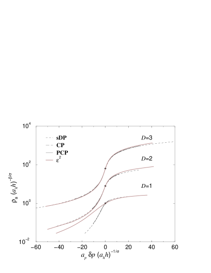
Figure 25: The universal scaling function ${\tilde{R}}(x,1)$ of the directed percolation universality class in various dimensions. The two- and three-dimensional data are vertically shifted by a factor $8$ and $64$ in order to avoid overlaps. The circles mark the condition ${\tilde{R}}(0,1)=1$. The gray lines correspond to an $\epsilon$-expansion of a renormalization group approach [181].

The universal scaling function ${\tilde{R}}(x,1)$ is displayed in Figure 25 for $D=1,2,3$. For each dimension, the data of the site directed percolation process, of the contact process as well as of the pair contact process collapse onto the unique scaling function. As expected the scaling functions vary with the spatial dimensionality below $D_{\scriptscriptstyle\mathrm{c}}$.

Similar to equilibrium the powerful and versatile $\epsilon$-expansion provides estimates for almost all quantities of interest (see page 15), in particular for the critical exponents [23, 178, 179, 180] and for the equation of state [181, 223]. Using a parametric representation [224, 225] of the directed percolation phase transition Janssen et al. showed that the equation of state is given within the $\epsilon^{2}$-approximation by the remarkable simple scaling function [181]

$$H(\theta)\;=\;\theta\,(2-\theta)+{\mathcal{O}}(\epsilon^{3})\,.$$ (3.57)

Here the scaling behavior of the quantities $\rho_{\scriptscriptstyle\mathrm{a}}$, $\delta p$, and $h$ is transformed to the variables $R$ and $\theta$ through the relations

$$b\,\delta p\;=\;R\,(1-\theta),\quad\quad\quad\rho_{\scriptscriptstyle\mathrm{a}}\;=\;R^{\beta}\,\frac{\theta}{2}\,.$$ (3.58)

The equation of state is given by

$$a\,h\;=\;\left(\frac{R^{\beta}}{2}\right)^{\delta}\;H(\theta)$$ (3.59)

with the metric factors $a$ and $b$. The whole phase diagram is described by the parameter range $R\geq 0$ and $\theta\in[0,2]$.

Figure 26: The universal scaling functions of the fluctuations ${\tilde{D}}(x,1)$ (left) and of the susceptibility ${\tilde{\mathrm{X}}}(x,1)$ (right) in various dimensions. The two- and three-dimensional fluctuation data are vertically shifted by a factor $8$ and $64$ in order to avoid overlaps. The circles mark the condition ${\tilde{D}}(0,1)=1$. In case of the susceptibility the two- and three-dimensional data are vertically shifted by a factor $3/2$ and $9/4$ in order to avoid overlaps. The circles mark the condition ${\tilde{\mathrm{X}}}(0,1)=\beta/\sigma$ and reflect the accuracy of the performed analysis.

Compared to the Widom-Griffiths scaling form [Eq. (3.17)] the parametric representation is not restricted to sufficiently small scaling arguments in the absorbing phase. The scaling function ${\tilde{R}}(x,1)$ can be calculated from the equation above, and the results are compared to the numerical data in Figure 25. As expected, the differences increase with increasing perturbation parameter $\epsilon$, i.e., with decreasing dimension and are especially strong in $D=1$ [140]. Thus higher orders than ${\mathcal{O}}(\epsilon^{2})$ are necessary to describe the scaling behavior of directed percolation in low dimensions. A more detailed discussion of the accuracy of the renormalization group data will be presented in 3.2.4.

The universal scaling functions of the order parameter fluctuations and the order parameter susceptibility are shown in Figure 26. The susceptibility is obtained by performing the numerical derivative of the order parameter with respect to the conjugated field. The perfect data-collapses confirm the scaling forms Eqs. (3.38-3.39). All scaling functions exhibit for $D=1,2,3$ a clear maximum signalling the divergence of $\Delta\rho_{\scriptscriptstyle\mathrm{a}}$ and $\chi$ at the critical point. The susceptibility data fulfills Eq. (3.52), reflecting the accuracy of the performed analysis. In summary all considered models are characterized by the same critical exponents and the same steady state scaling functions ${\tilde{R}}$, ${\tilde{D}}$, and ${\tilde{\mathrm{X}}}$. Thus the models are characterized by the same scaling behavior for $D=1,2,3$.

3.2.2 Above the upper critical dimension

According to the renormalization group scenario the stable fixed point of the recursion relations for $D>D_{\scriptscriptstyle\mathrm{c}}$ is usually the trivial fixed point with classical, i.e., mean field universal quantities. Thus, in contrast to the situation below $D_{\scriptscriptstyle\mathrm{c}}$ the critical exponents as well as the universal scaling functions are independent of the particular value of the dimension for $D>D_{\scriptscriptstyle\mathrm{c}}$. In most cases it is possible to derive these mean field exponents and even the scaling functions exactly since correlations and fluctuations can be neglected above $D_{\scriptscriptstyle\mathrm{c}}$. The mean field behavior of the contact process and the Domany-Kinzel automaton was considered in section 2.1 and in section 3.1.2, respectively. A corresponding analysis of the pair contact process can be found in [140]. The obtained universal scaling functions are given by (see e.g. [116])

$${\tilde{R}}_{\scriptscriptstyle\mathrm{MF}}(x,y) = \frac{x}{2}\,+\,\sqrt{y\,+\,\left(\frac{x}{2}\right)^{2}\;}\,,$$ (3.60)

$${\tilde{D}}_{\scriptscriptstyle\mathrm{MF}}(x,y) = \frac{{\tilde{R}}_{\scriptscriptstyle\mathrm{MF}}(x,y)}{\,{\sqrt{y\,+\,\left({x}/{2}\right)^{2}\;}}\,}\,,$$ (3.61)

$${\tilde{\mathrm{X}}}_{\scriptscriptstyle\mathrm{MF}}(x,y) = \frac{1}{\,2\,\,{\sqrt{y\,+\,\left({x}/{2}\right)^{2}\;}}\,}\,$$ (3.62)

$${\tilde{\Xi}}_{\raisebox{0.0pt}{$\scriptscriptstyle\perp$},\scriptscriptstyle\mathrm{MF}}(x,y) = \frac{1}{\,{\sqrt[4]{y\,+\,\left({x}/{2}\right)^{2}\;}}\,}\,$$ (3.63)

$${\tilde{\Xi}}_{\raisebox{0.0pt}{$\scriptscriptstyle\parallel$},\scriptscriptstyle\mathrm{MF}}(x,y) = \frac{1}{\,{\sqrt{y\,+\,\left({x}/{2}\right)^{2}\;}}\,}\,$$ (3.64)

yieldling the mean field exponents $\beta_{\scriptscriptstyle\mathrm{MF}}=1$, $\sigma_{\scriptscriptstyle\mathrm{MF}}=2$, $\gamma_{\scriptscriptstyle\mathrm{MF}}=1$, $\gamma^{\prime}_{\scriptscriptstyle\mathrm{MF}}=0$, $\nu_{\raisebox{0.0pt}{$\scriptscriptstyle\perp$},{\scriptscriptstyle\mathrm{MF}}}=1/2$, and $\nu_{\raisebox{0.0pt}{$\scriptscriptstyle\parallel$},{\scriptscriptstyle\mathrm{MF}}}=1$. These functions obey the scaling forms Eqs. (3.53-3.55).

Figure 27: The universal scaling function of the order parameter ${\tilde{R}}(x,1)$ (left) and the fluctuations ${\tilde{D}}(x,1)$ (right) for $D=5$. The five-dimensional data agree with the corresponding mean field functions Eq. (3.70) and Eq. (3.71), respectively.

The scaling behavior of the fluctuations deserves comment. The exponent $\gamma^{\prime}_{\scriptscriptstyle\mathrm{MF}}=0$ corresponds to a jump of the fluctuations and the scaling form Eq. (3.38) reduces to

$$a_{\scriptscriptstyle\Delta}\;\Delta\rho_{\scriptscriptstyle\mathrm{a}}(\delta p,h)\;\sim\;{\tilde{D}}_{\scriptscriptstyle\mathrm{MF}}(a_{\scriptscriptstyle p}\delta p\;\lambda,a_{\scriptscriptstyle h}h\,\lambda^{\sigma})\,.$$ (3.65)

Using again ${\tilde{D}}_{\scriptscriptstyle\mathrm{MF}}(0,1)=1$, the non-universal metric factor $a_{\scriptscriptstyle\Delta}$ is determined by

$$a_{\scriptscriptstyle\Delta}\;=\;\frac{1}{\,\Delta\rho_{\scriptscriptstyle\mathrm{a}}(\delta p=0,h)\,}\,.$$ (3.66)

The reduced scaling form Eq. (3.65) implies some interesting properties of the universal function ${\tilde{D}}_{\scriptscriptstyle\mathrm{MF}}$. The value ${\tilde{D}}_{\scriptscriptstyle\mathrm{MF}}(1,0)$ is now given by

$${\tilde{D}}_{\scriptscriptstyle\mathrm{MF}}(1,0)\;=\;\frac{\,\Delta\rho_{\scriptscriptstyle\mathrm{a}}(\delta p,h=0)\,}{\,\Delta\rho_{\scriptscriptstyle\mathrm{a}}(\delta p=0,h)\,}\,,$$ (3.67)

and the mean field scaling function fulfills the symmetries

$${\tilde{D}}_{\scriptscriptstyle\mathrm{MF}}(1,x) = {\tilde{D}}_{\scriptscriptstyle\mathrm{MF}}(x^{-1/\sigma},1)\,,$$ (3.68)

$${\tilde{D}}_{\scriptscriptstyle\mathrm{MF}}(x,1) = {\tilde{D}}_{\scriptscriptstyle\mathrm{MF}}(1,x^{-\sigma})\,,$$ (3.69)

for $x>0$. In particular we obtain for $x\to 0$ ${\tilde{D}}_{\scriptscriptstyle\mathrm{MF}}(1,0)={\tilde{D}}_{\scriptscriptstyle\mathrm{MF}}(\infty,1)$ and ${\tilde{D}}_{\scriptscriptstyle\mathrm{MF}}(0,1)={\tilde{D}}_{\scriptscriptstyle\mathrm{MF}}(1,\infty)$, respectively. This symmetry is an artefact of the zero fluctuation exponent and does not occur below the upper critical dimension. Therefore, it can be used to check whether a given $D$-dimensional system exhibits mean field behavior.

Numerical data of the five-dimensional models are presented in Figure 27. A good data-collapse of the rescaled data with the universal mean field scaling functions

$${\tilde{R}}_{\scriptscriptstyle{\mathrm{MF}}}(x,1) = \frac{x}{2}\,+\,\sqrt{1\,+\,\left(\frac{x}{2}\right)^{2}\;}\,$$ (3.70)

$${\tilde{D}}_{\scriptscriptstyle{\mathrm{MF}}}(x,1) = 1\,+\,\frac{x}{\,2\;\sqrt{1\,+\,\left({x}/{2}\right)^{2}\;}\,}\,$$ (3.71)

is obtained. The observed mean field behavior for $D=5$ agrees with the renormalization group result $D_{\scriptscriptstyle\mathrm{c}}=4$ [226, 103].

Figure 28: The universal Widom-Griffiths scaling function ${\tilde{H}}(x,1)$ for various dimensions as a function of $x=a_{\scriptscriptstyle p}\rho_{\scriptscriptstyle\mathrm{a}}^{-1/\beta}$. The numerically obtained curves ${\tilde{H}}(x,1)$ tend to the mean field result (long dashed lines) ${\tilde{H}}_{\scriptscriptstyle\mathrm{MF}}(x,1)=1-x$ with increasing dimension.

As already pointed out the scaling functions depend on the spatial dimension below $D_{\scriptscriptstyle\mathrm{c}}$. In particular the Widom-Griffiths scaling form [Eq. (3.43)] is well suited to examine how the universal functions approach the mean field solution with increasing dimension. The mean field Widom-Griffiths scaling form is given by

$${\tilde{H}}_{\scriptscriptstyle\mathrm{MF}}(x,y)\;=\;y^{2}\,-\,x\,y\,.$$ (3.72)

The rescaled field $a_{\scriptscriptstyle h}h\,\rho_{\scriptscriptstyle\mathrm{a}}^{-\sigma/\beta}$ is plotted in Figure 28 as a function of the rescaled control parameter $a_{\scriptscriptstyle p}\delta p\,\rho_{\scriptscriptstyle\mathrm{a}}^{-1/\beta}$. As can be seen the scaling functions ${\tilde{H}}(x,1)$ tend to the mean field curve ${\tilde{H}}_{\scriptscriptstyle\mathrm{MF}}(x,1)=1-x$ with increasing dimension. The observed agreement of the data of the five-dimensional models with the mean field scaling function ${\tilde{R}}_{\scriptscriptstyle\mathrm{MF}}$, ${\tilde{H}}_{\scriptscriptstyle\mathrm{MF}}$, and ${\tilde{D}}_{\scriptscriptstyle\mathrm{MF}}$ leads to the result that the upper critical dimension is less than five. This is a non-trivial result. The value of $D_{\scriptscriptstyle\mathrm{c}}$ is often predicted by field theoretical treatments, and a reliable determination of the upper critical dimension is therefore of particular interest. For example, two contrary field theories conjecture for the pair contact process $D_{\scriptscriptstyle\mathrm{c}}=4$ [198] and $D_{\scriptscriptstyle\mathrm{c}}=6$ [199, 200], respectively. The latter result is in clear contradiction to the observed mean field behavior in $D=5$. In this way, an upper bound on $D_{\scriptscriptstyle\mathrm{c}}$ can be obtained just by checking whether the numerical or experimental data are consistent with the usually known universal mean scaling functions.

3.2.3 At the upper critical dimension

The scaling behavior around the upper critical dimension $D_{\scriptscriptstyle\mathrm{c}}$ is well understood within the renormalization group theory (see for instance [22, 73, 17]). For $D>D_{\scriptscriptstyle\mathrm{c}}$ the stable fixed point of the corresponding renormalization equations is usually a trivial fixed point with mean field exponents. This trivial fixed point is unstable for $D<D_{\scriptscriptstyle\mathrm{c}}$, and a different stable fixed point exists with nonclassical exponents. For $D=D_{\scriptscriptstyle\mathrm{c}}$ both fixed points are identical and marginally stable. In this case, the scaling behavior is characterized by mean field power-laws modified by logarithmic corrections. For instance the order parameter is expected to obey in leading order

$$\rho_{\scriptscriptstyle\mathrm{a}}(\delta p,h=0) \,{\tilde{\propto}}\, \delta p\;|\ln{\delta p}|^{\mathrm{B}}\,,$$ (3.73)

$$\rho_{\scriptscriptstyle\mathrm{a}}(\delta p=0,h) \,{\tilde{\propto}}\, \sqrt{h}\;|\ln{h}|^{\Sigma}\,.$$ (3.74)

Greek capitals will be used in the following to denote the logarithmic correction exponents. These logarithmic correction exponents are characteristic features of the whole universality class similar to the usual critical exponents. Numerous theoretical, numerical, as well as experimental investigations of critical systems at the upper critical dimension have been performed (see for example [227, 228, 229, 230, 231, 232, 233, 234, 235, 236, 237, 238, 239, 141, 142, 223, 240, 241, 242, 243]). Logarithmic corrections make the data analysis notoriously difficult. Hence, most investigations focus on the determination of the correction exponents only, lacking the determination of the scaling functions at $D_{\scriptscriptstyle\mathrm{c}}$. Recent numerical [141, 242] as well as analytical results [223] reveal that the concept of universal scaling functions can also be applied to the upper critical dimension.

A method of analysis to determine both the universal scaling functions and the correction exponents at the upper critical dimension was developed in [141] and successfully applied to site directed percolation [142]. In this work the following phenomenological scaling ansatz is used for the Hankel-Stanley form of the equation of state (all terms in leading order)

$$a_{\scriptscriptstyle\mathrm{a}}\,\rho_{\scriptscriptstyle\mathrm{a}}(\delta p,h)\;\sim\;\lambda^{-\beta_{\scriptscriptstyle\mathrm{MF}}}\,|\ln{\lambda}|^{\Lambda}\;\;{\tilde{R}}(a_{\scriptscriptstyle p}\delta p\;\lambda\,|\ln{\lambda}|^{\Pi},a_{\scriptscriptstyle h}h\;\lambda^{\sigma_{\scriptscriptstyle\mathrm{MF}}}\,|\ln{\lambda}|^{\mathrm{H}})\,.$$ (3.75)

According to this scaling form, the order parameter at zero field ($h=0$) and at the critical density ($\delta p=0$) is given by

$$a_{\scriptscriptstyle\mathrm{a}}\,\rho_{\scriptscriptstyle\mathrm{a}}(\delta p,h=0) \sim a_{\scriptscriptstyle p}\,\delta p\;\;|\ln{a_{\scriptscriptstyle p}\delta p}|^{\mathrm{B}}\;\;{\tilde{R}}(1,0),$$ (3.76)

$$a_{\scriptscriptstyle\mathrm{a}}\,\rho_{\scriptscriptstyle\mathrm{a}}(\delta p=0,h) \sim \sqrt{a_{\scriptscriptstyle h}h}\;\,|\ln{\sqrt{a_{\scriptscriptstyle h}h}}|^{\Sigma}\;\;{\tilde{R}}(0,1)$$ (3.77)

with ${\mathrm{B}}=\Pi+\Lambda$ and $\Sigma={\mathrm{H}}/2+\Lambda$. Similar to $D\neq D_{\scriptscriptstyle\mathrm{c}}$ the normalization ${\tilde{R}}(0,1)={\tilde{R}}(1,0)=1$ is used. Furthermore, the scaling behavior of the equation of state is given in leading order by

$$a_{\scriptscriptstyle\mathrm{a}}\,\rho_{\scriptscriptstyle\mathrm{a}}(\delta p,h)\;\sim\;\sqrt{a_{\scriptscriptstyle h}h}\;|\ln{\sqrt{a_{\scriptscriptstyle h}h}}|^{\Sigma}\;\;{\tilde{R}}(x,1)$$ (3.78)

where $x$ denotes the scaling argument

$$x\;=\;a_{\scriptscriptstyle p}\delta p\,\sqrt{a_{\scriptscriptstyle h}h\,}^{\,-1}\,|\ln{\sqrt{a_{\scriptscriptstyle h}h}\,}|^{\Psi}$$ (3.79)

with $\Psi=\Pi-{\mathrm{H}}/2={\mathrm{B}}-\Sigma$.

In case of directed percolation it is possible to confirm the scaling form Eq. (3.75) by a renormalization group analysis [223], yielding in addition the values $\Lambda=7/12$, $\Pi=-1/4$, and ${\mathrm{H}}=-1/2$. Thus the scaling behavior of the equation of state is determined by

$${\mathrm{B}}\;=\;\Sigma\;=\;1/3\,,\quad\quad\quad\Psi=0\,.$$ (3.80)

It is worth mentioning that in contrast to the renormalization group results below the upper critical dimension, the logarithmic correction exponents do not rely on approximation schemes like $\epsilon$- or $1/n$-expansions. Within the RG theory they are exact results.

Figure 29: The universal scaling functions of the order parameter (upper left) and its fluctuations (upper right) at the upper critical dimension $D_{\scriptscriptstyle\mathrm{c}}=4$. The logarithmic correction exponents are given by ${\mathrm{B}}=\Sigma=1/3$ [223] and $\Psi=0$. For both models considered, the scaling plots contain at least three different curves corresponding to three different field values. The circles mark the condition ${\tilde{R}}(0,1)=1$ and ${\tilde{D}}(0,1)=1$, respectively. The lower figures show the order parameter for zero-field (left) and at the critical control parameter (right), respectively. The order parameter is rescaled according to Eq. (3.76) and Eq. (3.77). Approaching the transition point ($h\to 0$ and $\delta p\to 0$) the data tend to the function $f(x)=x$ (dashed lines) as required (see text).

Similarly to the order parameter the following scaling form is used for the fluctuations [141]

$$a_{\scriptscriptstyle\Delta}\;\Delta\rho_{\scriptscriptstyle\mathrm{a}}(\delta p,h)\;\sim\;\lambda^{\gamma^{\prime}_{\scriptscriptstyle\mathrm{MF}}}\;|\ln{\lambda}|^{\mathrm{K}}\;\;{\tilde{D}}(a_{\scriptscriptstyle p}\delta p\;\lambda\;|\ln{\lambda}|^{\Pi},a_{\scriptscriptstyle h}h\;\lambda^{-\sigma}\,|\ln{\lambda}|^{\mathrm{H}})\,.$$ (3.81)

Using the mean field value $\gamma^{\prime}_{\scriptscriptstyle\mathrm{MF}}=0$ and taking into account that numerical simulations show [142] that the fluctuations remain finite at the critical point (i.e. ${\mathrm{K}}=0$) the scaling form

$$a_{\scriptscriptstyle\Delta}\;\Delta\rho_{\scriptscriptstyle\mathrm{a}}(\delta p,h)\;\sim\;\;{\tilde{D}}(x,1)$$ (3.82)

is obtained, where the scaling argument $x$ is given by Eq. (3.79) with $\Psi=0$. The non-universal metric factor $a_{\scriptscriptstyle\Delta}$ is determined again by the condition ${\tilde{D}}(0,1)=1$.

In that way, the scaling behavior of the order parameter and its fluctuations at $D_{\scriptscriptstyle\mathrm{c}}$ is characterized by two exponents (${\mathrm{B}}=1/3$ and $\Sigma=1/3$) and four unknown non-universal metric factors ($a_{\scriptscriptstyle\mathrm{a}},a_{\scriptscriptstyle p},a_{\scriptscriptstyle h},a_{\scriptscriptstyle\Delta}$). Following [141] these values are determined by several conditions which are applied simultaneously: first, both the rescaled order parameter and the rescaled fluctuation data have to collapse to the universal functions ${\tilde{R}}(x,1)$ and ${\tilde{D}}(x,1)$. Second, the order parameter behavior at zero field and at the critical density is asymptotically given by the simple function $f(x)=x$ when plotting $[a_{\scriptscriptstyle\mathrm{a}}\rho_{\scriptscriptstyle\mathrm{a}}(\delta p,0)/a_{\scriptscriptstyle\rho}\delta p]^{1/{\mathrm{B}}}$ vs. $|\ln{a_{\scriptscriptstyle p}\delta p}|$ and $[a_{\scriptscriptstyle\mathrm{a}}\rho_{\scriptscriptstyle\mathrm{a}}(0,h)/\sqrt{a_{\scriptscriptstyle h}h\,}]^{1/{\Sigma}}$ vs. $|\ln{\sqrt{a_{\scriptscriptstyle h}h\,}}|$, respectively. Applying this analysis to data of both the contact process and site directed percolation, convincing results are obtained for ${\mathrm{B}}=\Sigma=1/3$, $\Psi=0$, and for the values of the non-universal metric factors listed in [142, 143]. The corresponding plots are presented in Figure 29 and show that the concept of universal scaling functions can be applied to the upper critical dimension.

Notice that no data-collapse is obtained if logarithmic corrections are neglected, i.e., for $\mathrm{B}=\Sigma=0$. Thus, the leading logarithmic corrections have to be taken into account in order to study steady state scaling functions. It is therefore remarkable that recently performed off-lattice simulations of the dynamical scaling behavior at $D_{\scriptscriptstyle\mathrm{c}}=4$ reveals that logarithmic corrections of higher orders (e.g. ${\mathcal{O}}({\ln{\ln{t}}})$) are necessary to describe the numerical data [244]. Although the steady state results presented here are quite convincing, we expect that even better results are obtained by incorporation higher order corrections. But in contrast to the dynamical scaling behavior, no analytical results of higher logarithmic corrections for the steady state scaling behavior are available so far.

3.2.4 Universal amplitude combinations

Additionally to the critical exponents and universal scaling functions, a universality class is also characterized by various universal amplitude combinations [68, 245]. These amplitude combinations emerge from the universality of the scaling functions since universal amplitude combinations correspond to particular values of the scaling functions. It is known from critical equilibrium systems that universal amplitude combinations vary usually more widely than the critical exponents. Thus these amplitude combinations are very useful in order to identify the universality class of a phase transition or to provide additional and often convincing evidence for the universal behavior. Furthermore, the measurement of amplitude combinations in experiments or simulations yields a reliable test for theoretical predictions. In particular, approximation schemes of the renormalization group, such as $\epsilon$- or $1/n$-expansions, are widely used to obtain explicit and systematic estimates of the amplitude combinations (see section 1.4).

Usually numerical investigations focus on amplitude combinations arising from finite-size scaling analyses (see e.g. [245]). A well known example is the value of Binder’s fourth order cumulant at criticality (see e.g. [112]). Instead of those finite-size properties we focus our attention on bulk critical behavior since bulk amplitude combinations are of great experimental interest. Furthermore, they can be compared to the renormalization group results of Janssen et al. [181].

The amplitude combination considered first is related to the susceptibility behavior below and above the transition. In analogy to equilibrium (see 1.3) the susceptibility diverges as

$$\chi(\delta p>0,h=0) \sim a_{\scriptscriptstyle\chi,+}\;\delta p^{-\gamma}\,,$$ (3.83)

$$\chi(\delta p<0,h=0) \sim a_{\scriptscriptstyle\chi,-}\;(-\delta p)^{-\gamma}\,,$$ (3.84)

if the critical point is approached from above and below, respectively. Using the scaling form Eq. (3.39) the susceptibility ratio

$$\frac{\,\chi(\delta p>0,h)\,}{\chi(\delta p<0,h)}\;=\;\left.\frac{\,{\tilde{\mathrm{X}}}(\phantom{-}a_{\scriptscriptstyle p}\delta p\;\lambda,a_{\scriptscriptstyle h}h\,\lambda^{\sigma})\,}{\,{\tilde{\mathrm{X}}}(-a_{\scriptscriptstyle p}\delta p\;\lambda,a_{\scriptscriptstyle h}h\,\lambda^{\sigma})\,}\,\right|_{a_{\scriptscriptstyle p}|\delta p|\lambda=1}\;=\;\frac{\,{\tilde{\mathrm{X}}}(+1,x)\,}{\,{\tilde{\mathrm{X}}}(-1,x)\,}$$ (3.85)

is clearly a universal quantity for all values of the scaling argument $x=a_{\scriptscriptstyle h}h|a_{\scriptscriptstyle p}\delta p|^{-\sigma}$. In particular it equals the ratio ${a_{\scriptscriptstyle\chi,+}}/{a_{\scriptscriptstyle\chi,-}}$ for vanishing field

$$\frac{\,a_{\scriptscriptstyle\chi,+}\,}{a_{\scriptscriptstyle\chi,-}}\;=\;\lim_{h\to 0}\,\frac{\,{\tilde{\mathrm{X}}}(+1,x)\,}{\,{\tilde{\mathrm{X}}}(-1,x)\,}\;=\;\frac{\,{\tilde{\mathrm{X}}}(+1,0)\,}{\,{\tilde{\mathrm{X}}}(-1,0)\,}\,.$$ (3.86)

In case of the mean field approximation Eq. (3.62) leads to

$$\frac{{\,\tilde{\mathrm{X}}}_{\scriptscriptstyle{\mathrm{MF}}}(+1,x)\,}{{\tilde{\mathrm{X}}}_{\scriptscriptstyle{\mathrm{MF}}}(-1,x)}\;=\;1$$ (3.87)

for all $x$. The susceptibility ratio ${\tilde{\mathrm{X}}}(+1,x)/{\tilde{\mathrm{X}}}(-1,x)$ is shown in Figure 30 for various models and different dimensions. The five dimensional data agree well with the mean field prediction. For $D<D_{\scriptscriptstyle\mathrm{c}}$ the ratio reflects the crossover from mean field to non-mean field behavior. Far away from the transition point, the critical fluctuations are suppressed and the behavior of the system is well described by the mean field solution. Approaching criticality, the critical fluctuations increase and a crossover to the $D$-dimensional behavior takes place.

Figure 30: The universal scaling function ${\tilde{\mathrm{X}}}(1,x)/{\tilde{\mathrm{X}}}(-1,x)$ for various dimensions and models. Site directed percolation data are marked by closed symbols. Open symbols correspond to data of the pair contact process for $D=2$ and to data of the contact process for $D=3$ and $D=5$, respectively. The dashed lines correspond to an $\epsilon$-expansion of a renormalization group approach [181]. The universal amplitude ${\tilde{\mathrm{X}}}(1,0)/{\tilde{\mathrm{X}}}(-1,0)$ is obtained from the extrapolation $a_{\scriptscriptstyle h}h|a_{\scriptscriptstyle p}\,\delta p|^{-\sigma}\to 0$.

A parametric representation of the susceptibility and therefore of the susceptibility ratio ${\tilde{\mathrm{X}}}(+1,x)/{\tilde{\mathrm{X}}}(-1,x)$ is derived in [181]. It is instructive to compare these results to the numerical data (see Fig. 30) since the theoretical curve reflects the accuracy of the RG estimations of all involved quantities, the exponent, the scaling functions, as well as the non-universal metric factors [142]. The perfect agreement between the numerical data and the RG curve for $D=3$ indicates that all quantities are approximated well. In the two-dimensional case a horizontal shift is observed between the numerical data and the RG-estimates. Thus the RG-approach yields good estimates for the exponents and the scaling functions, but the metric factors are of significantly less quality. For $D=1$ the $\epsilon^{2}$-approximation does not provide appropriate estimates of the DP scaling behavior similar to the equation of state (see Figure 25).

The consideration of the zero-field universal amplitude ratio ${\tilde{\mathrm{X}}}(+1,0)/{\tilde{\mathrm{X}}}(-1,0)$ offers a more quantitative check of the renormalization group results. Numerically this ratio is obtained by an extrapolation of the susceptibility ratio ${\tilde{\mathrm{X}}}(+1,x)/{\tilde{\mathrm{X}}}(-1,x)$ to $x\to 0$. The estimated values are listed in Table 1. Within the $\epsilon^{2}$-expansion this amplitude ratio is given by

$$\frac{{\tilde{\mathrm{X}}}(+1,0)}{\,{\tilde{\mathrm{X}}}(-1,0)\,}\;=\;1\,-\,\frac{\epsilon}{\,3\,}\,\left[\,1\,-\,\left(\frac{11}{288}\,-\,\frac{53}{144}\,\ln{\frac{4}{3}}\,\right)\,\epsilon\,+\,{\mathcal{O}}(\epsilon^{2})\right]\,.$$ (3.88)

Despite of the negative and therefore unphysical results for $D=1$ the RG results agree well with the numerical data (see also Fig. 30). For example, the two-dimensional values differ only by $3\%$. That has to be compared to the difference of the critical exponents. For example the RG estimate of the order parameter exponent [Eq. (3.14)] differs for $D=2$ from the best known numerical value by $6\%$ (see Table 1). The similar accuracy of the critical exponent and of the amplitude combination is contrary to an observation from critical equilibrium systems where the exponents are usually calculated more accurately by $\epsilon$-expansions than universal amplitude combinations (see section 1.4 for an example, as well as [68]). A possible explanation is that the $\epsilon^{2}$-approximation yields for $\epsilon=1,2$ much better results for directed percolation than e.g. for the Ising model. This is also reflected by the $\epsilon$-approximations of the equation of state. The various forms of the equation of state are less complicated for directed percolation. In particular the parametric representation of the equation of state [Eq. (3.57)] is remarkably simple.

Figure 31: The universal scaling function ${\tilde{D}}(1,x)/{\tilde{D}}(-1,x)$ for various dimensions. Site directed percolation data are marked by closed symbols whereas open symbols correspond to data of the contact process. The dashed line corresponds to the mean field scaling behavior.

Analogous to the susceptibility the universal amplitude ratio of the fluctuations is given by

$$\frac{\Delta\rho_{\scriptscriptstyle\mathrm{a}}(\delta p>0,h)}{\Delta\rho_{\scriptscriptstyle\mathrm{a}}(\delta p<0,h)}\;=\;\frac{\,{\tilde{D}}(+1,x)\,}{\,{\tilde{D}}(-1,x)\,}$$ (3.89)

with $x=a_{\scriptscriptstyle h}h|a_{\scriptscriptstyle p}\delta p|^{-\sigma}$. In case of absorbing phase transitions this ratio diverges for vanishing field. For $\delta p<0$ the order parameter fluctuations are zero for $h=0$ (absorbing state) whereas the fluctuations remain finite above the transition ($\delta p>0$). Thus absorbing phase transitions are generally characterized by

$$\frac{\,{\tilde{D}}(+1,0)\,}{\,{\tilde{D}}(-1,0)\,}\;\to\;\infty.$$ (3.90)

In Figure 31 the fluctuation ratio is plotted as a function of the scaling variable $x$ for various dimensions and models. The fluctuation ratios diverge for $x\to 0$ in all dimensions. The one-dimensional system exhibits a particular behavior characterized by the minimum of the corresponding curve. The origin of this behavior is that for $D=2,3$ the universal scaling function ${\tilde{D}}(x,1)$ exhibits a maximum for $x>0$, whereas for $D=1$ it is located at $x<0$ (see Figure 26). In case of the five-dimensional data a perfect agreement is observed with the mean field behavior

$$\frac{\,{\tilde{D}}_{\scriptscriptstyle{\mathrm{MF}}}(+1,x)\,}{{\tilde{D}}_{\scriptscriptstyle{\mathrm{MF}}}(-1,x)}\;=\;\frac{\,\phantom{-\,}1\,+\,\sqrt{1+4x\,}\,}{\,-\,1\,+\,\sqrt{1+4x\,}\,}\;\;\mathop{\longrightarrow}\limits_{x\to 0}\;\;\frac{\,1+2x\,}{2x}\,.$$ (3.91)

Figure 32: The universal scaling function ${\tilde{\mathrm{X}}}(1,x)$ for various dimensions. The dashed lines correspond to an $\epsilon$-expansion of a renormalization group approach [181]. The universal amplitude $R_{\scriptscriptstyle\chi}$ is obtained from the extrapolation $a_{\scriptscriptstyle h}h(a_{\scriptscriptstyle p}\,\delta p)^{-\sigma}\to 0$.

Finally we consider the universal amplitude combination $R_{\chi}$ (see Eq. (1.49)) which can be defined in the notation of absorbing phase transitions by

$$R_{\chi}\;=\;a_{\scriptscriptstyle\chi,+}\;\,a_{\scriptscriptstyle h}^{-1}\;\,a_{\scriptscriptstyle p}^{\sigma-\beta}\,.$$ (3.92)

The scaling forms Eq. (3.37) and Eq. (3.39) lead to

$$R_{\chi}\;=\;{\tilde{\mathrm{X}}}(1,0)$$ (3.93)

which is obviously a universal quantity. In Figure 32 the scaling function ${\tilde{\mathrm{X}}}(1,x)$ is plotted as a function of $x=a_{\scriptscriptstyle h}h\,(a_{\scriptscriptstyle p}\,\delta p)^{-\sigma}$ for various dimensions below $D_{\scriptscriptstyle\mathrm{c}}$. The corresponding data saturates for $x\to 0$, and the obtained estimates are listed in Table 1. Compared to the universal amplitude combination ${\tilde{\mathrm{X}}}(1,0)/{\tilde{\mathrm{X}}}(-1,0)$ the estimates of $R_{\chi}$ are of less accuracy since the data are affected by the uncertainty of the exponent $\gamma$ and the uncertainties of the metric factors $a_{\scriptscriptstyle p}$, $a_{\scriptscriptstyle h}$ [142]. These uncertainties increase the error-bars significantly. But nevertheless the two- and three-dimensional data agree quite well with the RG-results of [181] whereas unphysical results are obtained again for $D=1$ from the $\epsilon^{2}$-expansion.

In this way the analysis of combinations of the universal scaling functions provides a detailed and instructive check of the accuracy of corresponding renormalization group results. Compared to critical equilibrium systems the $\epsilon^{2}$-expansion provides astonishingly accurate estimates of certain amplitude combinations for $\epsilon=1$ and $\epsilon=2$. The $\epsilon^{2}$-approximation fails only in low dimensions ($\epsilon=3$), i.e., here, higher orders than ${\mathcal{O}}(\epsilon^{2})$ are necessary to describe the scaling behavior of directed percolation.

3.2.5 Finite-size scaling behavior

So far simulation data are considered where the correlation length $\xi_{\raisebox{0.0pt}{$\scriptscriptstyle\perp$}}$ is small compared to the system size $L$. Thus, the data presented above do not suffer from finite-size effects, such as rounding and shifting of the anomalies. As pointed out in section 2.2.1, an appropriate method to study finite-size effects of absorbing phase transitions within the steady state is to examine the field-dependence of the quantities of interest at the critical value $\delta p=0$ for various system sizes (see Figure 10). Similar to critical equilibrium scaling theory (see [246] for a review), it is assumed that the system size enters the scaling forms [Eqs. (3.37-3.38)] as an additional scaling field

$$\rho_{\scriptscriptstyle\mathrm{a}}(\delta p,h,L)\; \sim \;\lambda^{-\beta}\,\,{\tilde{R}}_{\scriptscriptstyle\mathrm{pbc},\Box}(a_{\scriptscriptstyle p}\delta p\;\lambda,a_{\scriptscriptstyle h}h\;\lambda^{\sigma},a_{\scriptscriptstyle L}L\;\lambda^{-\nu_{\raisebox{0.0pt}{$\scriptscriptstyle\perp$}}})\,,$$ (3.94)

$$a_{\scriptscriptstyle\Delta}\,\Delta\rho_{\scriptscriptstyle\mathrm{a}}(\delta p,h,L)\; \sim \;\lambda^{\gamma^{\prime}}\,\,{\tilde{D}}_{\scriptscriptstyle\mathrm{pbc},\Box}(a_{\scriptscriptstyle p}\delta p\;\lambda,a_{\scriptscriptstyle h}h\,\lambda^{\sigma},a_{\scriptscriptstyle L}L\;\lambda^{-\nu_{\raisebox{0.0pt}{$\scriptscriptstyle\perp$}}})\,.$$ (3.95)

The choice of the corresponding scaling power $\nu_{\raisebox{0.0pt}{$\scriptscriptstyle\perp$}}$ is motivated by the phenomenological finite-size scaling theory which rests on the assumption that finite-size effects are controlled within the scaling regime by the ratio $L/\xi_{\raisebox{0.0pt}{$\scriptscriptstyle\perp$}}$ [247, 248]. Approaching the transition point, finite-size effects are expected to occur when ${\mathcal{O}}(\xi_{\raisebox{0.0pt}{$\scriptscriptstyle\perp$}})=L$. If both lengths, $L$ and $\xi_{\raisebox{0.0pt}{$\scriptscriptstyle\perp$}}$, are significantly larger than all other length scales of a given system (e.g. the lattice spacing) the above finite-size scaling forms are universal. Thus, they may be used to identify a system’s universality class, additionally to the so far considered scaling forms associated to the thermodynamic limit $L\to\infty$. For example, it was shown by the use of universal finite-size scaling functions that the liquid-gas phase transition of a Lennard-Jones system belongs to the Ising universality class [249, 250, 251, 252].

The index $\mathrm{pbc},\Box$ in Eq. (3.94) and Eq. (3.95) indicates that the universal finite-size scaling functions depend on the particular choice of the boundary conditions as well as on the system shape (see e.g. [253, 254, 255, 121, 256]). But different lattice structures are contained in the metric factor $a_{\scriptscriptstyle L}$. Throughout this work we focus on hypercubic lattices of size $L^{D}$ (aspect ratio $1$) with periodic boundary conditions (pbc). Of course, the universal scaling functions Eqs. (3.37-3.38) are recovered in the thermodynamic limit, e.g.

$${\tilde{R}}_{\scriptscriptstyle\mathrm{pbc},\Box}(x,y,\infty)\;=\;{\tilde{R}}(x,y)\,.$$ (3.96)

Additionally to the order parameter and its fluctuations we consider the fourth-order cumulant $Q$ which is defined as (see e.g. [257, 112])

$$Q\;=\;1\,-\,\frac{\langle\rho_{\scriptscriptstyle\mathrm{a}}^{4}\rangle}{\,3\,\langle\rho_{\scriptscriptstyle\mathrm{a}}^{2}\rangle^{2}\,}\,.$$ (3.97)

Other combinations of order parameter moments can be constructed and were investigated for several systems exhibiting absorbing phase transitions [196, 205, 211, 245]. Here, we restrict our attention to $Q$ since the cumulant behavior is sufficient for our investigation [152]. For non-vanishing order-parameter the cumulant tends to $Q=2/3$ in the thermodynamic limit. In case of a zero order parameter the cumulant vanishes if the order parameter is characterized by a Gaussian distribution symmetrically distributed around zero. The latter case is observed in equilibrium systems, e.g. the Ising model for $T>T_{\scriptscriptstyle\mathrm{c}}$. But for absorbing phase transitions the order parameter is non-negative per definition. Thus the order parameter is characterized by a non-trivial distribution and the above scenario does not apply.

Nevertheless, it is expected that the cumulant obeys the scaling form

$$Q(\delta p,h,L)\;\sim\;{\tilde{Q}}_{\scriptscriptstyle\mathrm{pbc},\Box}(a_{\scriptscriptstyle p}\delta p\;\lambda,a_{\scriptscriptstyle h}h\;\lambda^{\sigma},a_{\scriptscriptstyle L}L\;\lambda^{-\nu_{\raisebox{0.0pt}{$\scriptscriptstyle\perp$}}})\,.$$ (3.98)

Notice that no metric factor $a_{\scriptscriptstyle Q}$ is introduced since the cumulant is already dimensionless. Choosing $a_{\scriptscriptstyle L}L\,\lambda^{-\nu_{\perp}}=1$ we find for zero field

$$Q(0,0,L) = \left.{Q}\vphantom{\tilde{Q}}(\delta p,0,L)\right|_{\scriptscriptstyle\delta p=0}$$ (3.99)

$$\sim \left.{\tilde{Q}}_{\scriptscriptstyle\mathrm{pbc},\Box}(a_{\scriptscriptstyle p}\delta p\;(a_{\scriptscriptstyle L}L)^{-\nu_{\perp}},0,1)\right|_{\scriptscriptstyle\delta p=0}$$

$$= {\tilde{Q}}_{\scriptscriptstyle\mathrm{pbc},\Box}(0,0,1)$$

which is universal despite of the boundary condition and the system shape. The universal value ${\tilde{Q}}_{\scriptscriptstyle\mathrm{pbc},\Box}(0,0,1)$ corresponds to an intersection point if one plots $Q$ as a function of the control parameter $p$ for various system sizes $L$. Thus it is possible to determine the critical value $p_{\scriptscriptstyle\mathrm{c}}$ from the common intersection point. This cumulant intersection method is very useful and was applied in numerous works (see for instance [112] and references therein). But as pointed out in section 2.2.1, it is a characteristic feature of absorbing phase transitions that the steady state order parameter moments $\langle\rho_{\scriptscriptstyle\mathrm{a}}^{k}\rangle$ vanish as soon as ${\mathcal{O}}(\xi_{\raisebox{0.0pt}{$\scriptscriptstyle\perp$}})=L$ even in the active phase. Thus the powerful cumulant intersection method can not be applied for absorbing phase transitions.

In order to bypass this problem we consider the cumulant as a function of the conjugated field for $\delta p=0$. It is convenient to norm the universal scaling function ${\tilde{Q}}_{\scriptscriptstyle\mathrm{pbc},\Box}$ by the condition

$${\tilde{Q}}_{\scriptscriptstyle\mathrm{pbc},\Box}(0,1,1)\;=\;0.$$ (3.100)

Since the metric factor $a_{\scriptscriptstyle h}$ is already known, the condition above can be used to determine the metric factor $a_{\scriptscriptstyle L}$. Taking into account that the spatial correlation length scales at criticality as [Eq. (3.41)]

$$a_{\raisebox{0.0pt}{$\scriptscriptstyle\perp$}}\,\xi_{\raisebox{0.0pt}{$\scriptscriptstyle\perp$}}\;\sim\;(a_{\scriptscriptstyle h}\,h)^{-\nu_{\raisebox{0.0pt}{$\scriptscriptstyle\perp$}}/\sigma}\,,$$ (3.101)

Eq. (3.100) implies that the universal function ${\tilde{Q}}_{\scriptscriptstyle\mathrm{pbc},\Box}$ is positive if $a_{\scriptscriptstyle L}L>a_{\raisebox{0.0pt}{$\scriptscriptstyle\perp$}}\,\xi_{\raisebox{0.0pt}{$\scriptscriptstyle\perp$}}$ and negative if $a_{\scriptscriptstyle L}L<a_{\raisebox{0.0pt}{$\scriptscriptstyle\perp$}}\,\xi_{\raisebox{0.0pt}{$\scriptscriptstyle\perp$}}$. Note that in case of equilibrium phase transitions Eq. (3.100) is useless since the cumulant is usually positive.

Figure 33: The universal finite-size scaling analysis for the directed percolation universality class in various dimensions. The filled circles mark the condition Eq. (3.100). The horizontal lines correspond to the cumulant limit $2/3$. The vertical lines separate the finite-size regime with $a_{\scriptscriptstyle L}L<a_{\raisebox{0.0pt}{$\scriptscriptstyle\perp$}}\,\xi_{\raisebox{0.0pt}{$\scriptscriptstyle\perp$}}$ (left) from the regime with $a_{\scriptscriptstyle L}L>a_{\raisebox{0.0pt}{$\scriptscriptstyle\perp$}}\,\xi_{\raisebox{0.0pt}{$\scriptscriptstyle\perp$}}$ (right). The data are obtained from simulations of systems sizes $L=64,128,256,512$ for $D=1$, $L=64,128,256$ for $D=2$, and $L=32,64,128$ for $D=3$.

As mentioned above we focus on the scaling behavior at $p=p_{\scriptscriptstyle\mathrm{c}}$ and investigate the universal scaling functions ${\tilde{R}}_{\scriptscriptstyle\mathrm{pbc},\Box}(0,x,1)$, ${\tilde{D}}_{\scriptscriptstyle\mathrm{pbc},\Box}(0,x,1)$, ${\tilde{Q}}_{\scriptscriptstyle\mathrm{pbc},\Box}(0,x,1)$, by plotting the rescaled quantities

$$\rho_{\scriptscriptstyle\mathrm{a}}(0,h,L)\;(a_{\scriptscriptstyle L}\,L)^{\beta/\nu_{\raisebox{0.0pt}{$\scriptscriptstyle\perp$}}}\,,\quad\quad a_{\scriptscriptstyle\Delta}\;\Delta\rho_{\scriptscriptstyle\mathrm{a}}(0,h,L)\;(a_{\scriptscriptstyle L}\,L)^{-\gamma^{\prime}/\nu_{\raisebox{0.0pt}{$\scriptscriptstyle\perp$}}}\,$$ (3.102)

and $Q(0,h,L)$ as a function of the rescaled field $x=a_{\scriptscriptstyle h}h(a_{\scriptscriptstyle L}L)^{\sigma/\nu_{\raisebox{0.0pt}{$\scriptscriptstyle\perp$}}}$. Obviously, only a horizontal rescaling is needed in order to produce a data-collapse of the cumulant data. Thus the determination of the critical exponent $\nu_{\raisebox{0.0pt}{$\scriptscriptstyle\perp$}}$ via the fourth order cumulant is more accurate than a corresponding analysis of the order parameter or of the fluctuations. Therefore cumulants are widely used in order to estimate the correlation length exponent. The finite-size scaling analysis of site directed percolation, of the contact process, and of the pair contact process is presented in Figure 33. Using the best known values for the critical exponent $\nu_{\raisebox{0.0pt}{$\scriptscriptstyle\perp$}}$ (see Table 1) perfect data-collapses are observed. Note that different lattice structures do not affect the universal scaling functions. Whereas bcc lattice types are used for site directed percolation, simples cubic lattices are used for the contact process and pair contact process. As can be seen the order parameter and its fluctuations obey the expected algebraic field dependence for $x\gg 1$, i.e., as long as $a_{\raisebox{0.0pt}{$\scriptscriptstyle\perp$}}\xi_{\raisebox{0.0pt}{$\scriptscriptstyle\perp$}}\ll a_{\scriptscriptstyle L}L$. The fluctuation curves are characterized by a clear maximum signalling its singular behavior in the thermodynamic limit. Approaching the transition point the fourth-order cumulant tends to minus infinity for all models in all dimensions

$${\tilde{Q}}_{\scriptscriptstyle{\mathrm{pbc},\Box}}(0,x,1)\;\longrightarrow\;-\infty\quad\quad{\mathrm{for}}\quad\quad x\;\to\;0\,.$$ (3.103)

This behavior is caused by the vanishing steady state fluctuations, and it is assumed that the divergent fourth-order cumulant is a characteristic feature of all absorbing phase transitions [152]. A ratio that remains finite at criticality is obtained via $U=({\langle\rho_{\scriptscriptstyle\mathrm{a}}^{2}\rangle\langle\rho_{\scriptscriptstyle\mathrm{a}}^{3}\rangle-\langle\rho_{\scriptscriptstyle\mathrm{a}}\rangle\langle\rho_{\scriptscriptstyle\mathrm{a}}^{2}\rangle^{2}})/({\langle\rho_{\scriptscriptstyle\mathrm{a}}\rangle\langle\rho_{\scriptscriptstyle\mathrm{a}}^{4}\rangle-\langle\rho_{\scriptscriptstyle\mathrm{a}}\rangle\langle\rho_{\scriptscriptstyle\mathrm{a}}^{2}\rangle^{2}})$ [258]. The value of $U$ for $x\to 0$ characterizes the universality class. Numerical investigations yield $U_{d=1}=0.833\raisebox{0.86108pt}{$\scriptstyle\pm$}0.011$, $U_{d=2}=0.704\raisebox{0.86108pt}{$\scriptstyle\pm$}0.013$, and $U_{d=3}=0.61\raisebox{0.86108pt}{$\scriptstyle\pm$}0.02$.

So far we considered the finite-size scaling behavior below the upper critical dimension $D_{\scriptscriptstyle\mathrm{c}}$. The situation becomes more complicated above $D_{\scriptscriptstyle\mathrm{c}}$ where the mean field theory applies. Naively, one would expect that the finite-size scaling behavior is described by the mean field exponents $\beta_{\scriptscriptstyle\mathrm{MF}}$, $\sigma_{\scriptscriptstyle\mathrm{MF}}$, and $\nu_{\raisebox{0.0pt}{$\scriptscriptstyle\perp$},{\scriptscriptstyle\mathrm{MF}}}$ and e.g. the order parameter obeys

$$\rho_{\scriptscriptstyle\mathrm{a}}(\delta p,h,L)\;\sim\;\lambda^{-\beta_{\scriptscriptstyle\mathrm{MF}}}\,\,{\tilde{R}}_{\scriptscriptstyle\mathrm{pbc},\Box}(a_{\scriptscriptstyle p}\delta p\;\lambda,a_{\scriptscriptstyle h}h\;\lambda^{\sigma_{\scriptscriptstyle\mathrm{MF}}},a_{\scriptscriptstyle L}L\;\lambda^{-\nu_{\raisebox{0.0pt}{$\scriptscriptstyle\perp$},{\scriptscriptstyle\mathrm{MF}}}})\,.$$ (3.104)

But as can be seen in Figure 34 for the order parameter cumulant no data-collapse occurs for $\nu_{\raisebox{0.0pt}{$\scriptscriptstyle\perp$},{\scriptscriptstyle\mathrm{MF}}}=1/2$ reflecting the failure of phenomenological finite scaling within the mean field regime (see [78] for a readable review). This breakdown of common finite-size scaling is well established in equilibrium although details are discussed controversially in the literature [259, 260, 261, 262, 263, 264, 265, 266, 267, 78]. As pointed out by Brézin on the basis of exact calculations in the limit $n\to\infty$, the usual finite-size scaling assumption breaks for $D\hskip 2.15277pt\raisebox{1.72218pt}{$\scriptstyle\geq$}\hskip 2.15277ptD_{\scriptscriptstyle\mathrm{c}}$ due to the existence of a dangerous irrelevant variable [79]. In that case, the above scaling forms are replaced by [260]

$$\rho_{\scriptscriptstyle\mathrm{a}}(\delta p,h,L)\;\sim\;\lambda^{-\beta_{\scriptscriptstyle\mathrm{MF}}}\,\,{\tilde{R}}_{\scriptscriptstyle\mathrm{pbc},\Box}(a_{\scriptscriptstyle p}\delta p\;\lambda,a_{\scriptscriptstyle h}h\;\lambda^{\sigma_{\scriptscriptstyle\mathrm{MF}}},a_{\scriptscriptstyle L}L\;\lambda^{-\nu_{\raisebox{0.0pt}{$\scriptscriptstyle\perp$},{\scriptscriptstyle\mathrm{MF}}}^{\ast}})\,.$$ (3.105)

The modified scaling form reflects that finite-size scaling above $D_{\scriptscriptstyle\mathrm{c}}$ is no longer controlled by the ratio $L/\xi\,{\tilde{\propto}}\,L|\delta p|^{\scriptscriptstyle\nu_{\raisebox{0.0pt}{$\scriptscriptstyle\perp$},{\scriptscriptstyle\mathrm{MF}}}}$ but by the ratio $L/l_{\scriptscriptstyle 0}$. In equilibrium, the so-called thermodynamic length $l_{\scriptscriptstyle 0}$ scales as [260]

$$l_{\scriptscriptstyle 0}\,\,{\tilde{\propto}}\,\,|\delta p|^{-(2\beta_{\scriptscriptstyle\mathrm{MF}}\,+\,\gamma_{\scriptscriptstyle\mathrm{MF}})/D}\,.$$ (3.106)

Below the upper critical dimension, the hyperscaling law $2\,\beta+\gamma=2-\alpha=\nu_{\raisebox{0.0pt}{$\scriptscriptstyle\perp$}}D$ holds and $l_{\scriptscriptstyle 0}$ coincides with the correlation length $\xi_{\raisebox{0.0pt}{$\scriptscriptstyle\perp$}}$. It is instructive to express the divergence of the thermodynamic length in terms of the value of the upper critical dimension $D_{\scriptscriptstyle\mathrm{c}}$.

Figure 34: The universal finite-size scaling analysis for the directed percolation universality class above the upper critical dimension. Using the standard finite-size scaling form with $\beta_{\scriptscriptstyle\mathrm{MF}}=1$, $\sigma_{\scriptscriptstyle\mathrm{MF}}=2$, and $\nu_{\raisebox{0.0pt}{$\scriptscriptstyle\perp$},{\scriptscriptstyle\mathrm{MF}}}=1/2$ no data-collapse occurs (left). Instead the finite-size scaling behavior is described by a modified scaling form using $\beta_{\scriptscriptstyle\mathrm{MF}}=1$, $\sigma_{\scriptscriptstyle\mathrm{MF}}=2$, and $\nu_{\raisebox{0.0pt}{$\scriptscriptstyle\perp$},{\scriptscriptstyle\mathrm{MF}}}^{\ast}=2/D$. The filled circles mark the condition Eq. (3.100). The vertical lines correspond to the cumulant limit $2/3$. The data are obtained from simulations of system sizes $L=8,16,32$ for site directed percolation and $L=4,8,16$ for the contact process. As can be seen in the right figure, the numerical data agree perfectly with the analytical result $Q=2/3\,(1-1/x)$ [268, 258].

According to the Ginzburg criterion (see chapter 5), its value is given in equilibrium by $D_{\scriptscriptstyle\mathrm{c}}=(2\beta_{\scriptscriptstyle\mathrm{MF}}+\gamma_{\scriptscriptstyle\mathrm{MF}})/\nu_{\raisebox{0.0pt}{$\scriptscriptstyle\perp$},{\scriptscriptstyle\mathrm{MF}}}$ leading to

$$\left.l_{\scriptscriptstyle 0}^{\vphantom{X}}\right|_{\scriptscriptstyle D>D_{\scriptscriptstyle\mathrm{c}}}\,\,{\tilde{\propto}}\,\,|\delta p|^{-\nu_{\raisebox{0.0pt}{$\scriptscriptstyle\perp$},{\scriptscriptstyle\mathrm{MF}}}D_{\scriptscriptstyle\mathrm{c}}/D}\,.$$ (3.107)

Thus, the scaling power of the finite-size scaling forms is given by

$$\nu_{\raisebox{0.0pt}{$\scriptscriptstyle\perp$},{\scriptscriptstyle\mathrm{MF}}}^{\ast}\;=\;\nu_{\raisebox{0.0pt}{$\scriptscriptstyle\perp$},{\scriptscriptstyle\mathrm{MF}}}\,\frac{\,D_{\scriptscriptstyle\mathrm{c}}}{\,D_{\phantom{\scriptscriptstyle c}}}\,.$$ (3.108)

For example, the short range interaction Ising model is characterized by $\nu_{\raisebox{0.0pt}{$\scriptscriptstyle\perp$},{\scriptscriptstyle\mathrm{MF}}}=1/2$ and $D_{\scriptscriptstyle\mathrm{c}}=4$ yielding $\nu_{\raisebox{0.0pt}{$\scriptscriptstyle\perp$},{\scriptscriptstyle\mathrm{MF}}}^{\ast}=2/D$. This value is derived by a renormalization group analysis [77] and is confirmed by numerical simulations [260, 262]. Furthermore, Eq. (3.108) also describes the modified finite-size scaling behavior of long-range interacting systems [259, 261]. In that case, the interactions decay as $r^{\scriptscriptstyle-(D+\sigma)}$ ($\sigma>2$ corresponds to short-range interacting systems), yielding the upper critical dimension $D_{\scriptscriptstyle\mathrm{c}}=2\sigma$ as well as $\nu_{\raisebox{0.0pt}{$\scriptscriptstyle\perp$},{\scriptscriptstyle\mathrm{MF}}}=1/\sigma$ [269, 270, 271, 272].

Analogous to the equilibrium scenario considered above, directed percolation exhibits a dangerous irrelevant variable within the mean field regime (the coupling constant $u$ in Eq. (3.8)), explaining the breakdown of usual finite-size scaling above $D_{\scriptscriptstyle\mathrm{c}}$. Following Eq. (3.108), the modified scaling form is characterized by the exponent

$$\nu_{\raisebox{0.0pt}{$\scriptscriptstyle\perp$},{\scriptscriptstyle\mathrm{MF}}}^{\ast}\;=\;\frac{2}{\,D\,}\,.$$ (3.109)

since $D_{\scriptscriptstyle\mathrm{c}}=4$ and $\nu_{\raisebox{0.0pt}{$\scriptscriptstyle\perp$},{\scriptscriptstyle\mathrm{MF}}}=1/2$. As can be seen in Figure 34, a perfect universal data-collapse is obtained if the data of the five-dimensional models are scaled with $\nu_{\raisebox{0.0pt}{$\scriptscriptstyle\perp$},{\scriptscriptstyle\mathrm{MF}}}^{\ast}=2/5$. Preliminary results show that corresponding data of two-dimensional absorbing phase transitions with infinite particle hopping collapse onto the same universal scaling curves if $\nu_{\raisebox{0.0pt}{$\scriptscriptstyle\perp$},{\scriptscriptstyle\mathrm{MF}}}^{\ast}=1$ is used. This indicates that Eq. (3.109) holds independently of the range of interactions. Furthermore, the exponent $\nu_{\raisebox{0.0pt}{$\scriptscriptstyle\perp$},{\scriptscriptstyle\mathrm{MF}}}^{\ast}$ is $D$-dependent and therefore non-universal, whereas the finite-size scaling functions are universal.

A recently performed field theoretical approach of the mean field scaling behavior of directed percolation confirms the analysis above. Similar to equilibrium [79, 78], a zero-momentum mode treatment allows to consider finite-size effects of periodic systems [273]. Within the mean field regime it is possible to calculate analytically the critical exponent $\sigma/\nu_{\raisebox{0.0pt}{$\scriptscriptstyle\perp$},{\scriptscriptstyle\mathrm{MF}}}^{\ast}=D$ [confirming Eq. (3.109)] as well as the scaling functions [268, 258]

$${\tilde{R}}_{\scriptscriptstyle\mathrm{pbc},\Box,\mathrm{mf}}(0,x,1) = \sqrt{2}\,\frac{\,\Gamma(\frac{x+1}{2})\,}{\Gamma(\frac{x}{2})}\,,$$ (3.110)

$${\tilde{Q}}_{\scriptscriptstyle\mathrm{pbc},\Box,\mathrm{mf}}(0,x,1) = \frac{2}{3}\,\left(1\,-\,\frac{1}{x}\right)\,.$$ (3.111)

As can be seen in Figure 34 the numerical data agree perfectly with the analytical results.

In conclusion, universal finite-scaling functions can be used additionally to the scaling behavior of the equation of state, the susceptibility, etc. to identify a system’s universality class. Analogous to equilibrium, simple finite-size scaling is valid below $D_{\scriptscriptstyle\mathrm{c}}$ but has to be modified within the mean field regime.

3.3 Dynamical scaling behavior

In this section we discuss the dynamical scaling behavior close to the transition point. First we consider how the order parameter decays starting from a fully occupied lattice, i.e., starting from a homogenous particle source. Second we investigate the activity spreading generated from a single active seed. Interpreting the initial particle density as another scaling field both scaling regimes are connected by a crossover scenario.

3.3.1 Homogeneous particle source

In section 2.2.2 we have seen that away from criticality the order parameter approaches its steady state value exponentially. At the critical point the order parameter decays algebraically

$$\rho_{\scriptscriptstyle\mathrm{a}}(t)\;\sim\;(a_{\scriptscriptstyle t}\,t)^{-\alpha}\,$$ (3.112)

where $a_{\scriptscriptstyle t}$ denotes the associated non-universal metric factor. The dynamical behavior of the order parameter can be incorporated in the scaling forms by an additional scaling field

$$\rho_{\scriptscriptstyle\mathrm{a}}(\delta p,h,L,t)\;\sim\;\lambda^{-\beta}\,\,{\tilde{R}}_{\scriptscriptstyle\mathrm{pbc},\Box,\mathrm{full}}(a_{\scriptscriptstyle p}\delta p\;\lambda,a_{\scriptscriptstyle h}h\;\lambda^{\sigma},a_{\scriptscriptstyle L}L\;\lambda^{-\nu_{\raisebox{0.0pt}{$\scriptscriptstyle\perp$}}},a_{\scriptscriptstyle t}t\;\lambda^{-\nu_{\raisebox{0.0pt}{$\scriptscriptstyle\parallel$}}})\,.$$ (3.113)

The scaling power of $t$ has to equal the scaling power of the correlation time $\xi_{\raisebox{0.0pt}{$\scriptscriptstyle\parallel$}}$, and the index full indicates the initial conditions. Setting $a_{\scriptscriptstyle t}t\;\lambda^{-\nu_{\raisebox{0.0pt}{$\scriptscriptstyle\parallel$}}}=1$ leads in the thermodynamic limit at criticality to

$$\rho_{\scriptscriptstyle\mathrm{a}}(\delta p=0,h=0,L\to\infty,t)\;\sim\;(a_{\scriptscriptstyle t}\,t)^{-\beta/\nu_{\raisebox{0.0pt}{$\scriptscriptstyle\parallel$}}}\;\,{\tilde{R}}_{\scriptscriptstyle\mathrm{pbc},\Box,\mathrm{full}}(0,0,\infty,1)\,.$$ (3.114)

Thus Eq. (3.112) is recovered for ${\tilde{R}}_{\scriptscriptstyle\mathrm{pbc},\Box,\mathrm{full}}(0,0,\infty,1)=1$ and the exponents $\alpha$, $\beta$, and $\nu_{\raisebox{0.0pt}{$\scriptscriptstyle\parallel$}}$ fulfill the scaling law

$$\alpha\;=\;\frac{\,\beta\,}{\nu_{\raisebox{0.0pt}{$\scriptscriptstyle\parallel$}}}\,.$$ (3.115)

A finite system size limits the power-law behavior above. The corresponding finite-size scaling form is obtained by choosing $a_{\scriptscriptstyle L}L\lambda^{-\nu_{\raisebox{0.0pt}{$\scriptscriptstyle\perp$}}}=1$

$$\rho_{\scriptscriptstyle\mathrm{a}}(\delta p=0,h=0,L,t)\;\sim\;(a_{\scriptscriptstyle L}L)^{-\beta/\nu_{\raisebox{0.0pt}{$\scriptscriptstyle\perp$}}}\,\,{\tilde{R}}_{\scriptscriptstyle\mathrm{pbc},\Box,\mathrm{full}}(0,0,1,a_{\scriptscriptstyle t}t\;(a_{\scriptscriptstyle L}L)^{-z})\,,$$ (3.116)

where $z=\nu_{\raisebox{0.0pt}{$\scriptscriptstyle\parallel$}}/\nu_{\raisebox{0.0pt}{$\scriptscriptstyle\perp$}}$ denotes the dynamical exponent. Finite-size effects have to be taken into account for

$${\mathcal{O}}(t)=t_{\scriptscriptstyle\mathrm{FSS}}\quad\quad\quad\mathrm{with}\quad\quad\quad t_{\scriptscriptstyle\mathrm{FSS}}=a_{\scriptscriptstyle t}^{-1}\,(a_{\scriptscriptstyle L}\,L)^{z}\,.$$ (3.117)

For $t\ll t_{\scriptscriptstyle\mathrm{FSS}}$ the scaling function obeys the power-law ${\tilde{R}}_{\scriptscriptstyle\mathrm{pbc},\Box,\mathrm{full}}(0,0,1,x)\sim x^{-\alpha}$, whereas ${\tilde{R}}_{\scriptscriptstyle\mathrm{pbc},\Box,\mathrm{full}}(0,0,1,x)$ decays exponentially for $x\gg 1$, i.e., $t\gg t_{\scriptscriptstyle\mathrm{FSS}}$. This is shown in Figure 35 where the raw data as well as the rescaled data are presented for $D=1$ and various system sizes. Again the data of all considered models collapse onto the single universal curve ${\tilde{R}_{\scriptscriptstyle\mathrm{pbc},\Box,\mathrm{full}}(0,0,1,x)}$. It is worth mentioning that the models are simulated with different update schemes. Whereas a parallel or synchronous update scheme is applied for site directed percolation, the contact process and the pair contact process are simulated with an asynchronous update, implemented by a random sequential update. The observed data-collapse confirms that different update schemes are contained in the non-universal metric factors $a_{\scriptscriptstyle t}$ and do not affect the universal scaling functions.

Figure 35: The order parameter decay at the critical point for $D=1$. The left figure shows the unscaled data of one-dimensional site directed percolation for $L=64,128,256$ (from left to right). Additionally to the order parameter $\rho_{\scriptscriptstyle\mathrm{a}}(t)$ the survival probability $P_{\scriptscriptstyle\mathrm{a}}(t)$ is presented in order to display the rapidity reversal symmetry ($\mu=\sqrt{2-p_{\scriptscriptstyle\mathrm{c}}\,}\,$). The rescaled data, i.e., the universal scaling function ${\tilde{R}(0,0,1,x)}$ [see Eq. (3.117)] is presented in the right figure for site directed percolation, the contact process and the pair contact process. The long-dashed line corresponds to the power-law behavior of the infinite system [Eq. (3.112)].

As already mentioned, the rapidity reversal of directed percolation implies the asymptotic equivalence of the survival probability and the order parameter decay at criticality [Eq. (3.12)]

$$P_{\scriptscriptstyle\mathrm{a}}(t)\;\sim\;\mu^{2}\,\rho_{\scriptscriptstyle\mathrm{a}}(t)\,.$$ (3.118)

The extension of the above dynamical scaling analysis to higher dimensions is redundant because a detailed analysis of the survival probability will be presented in the next section. But a comment about the rapidity reversal symmetry for site directed percolation is worth making. The order parameter $\rho_{\scriptscriptstyle\mathrm{a}}(t)$ as well as the survival probability $P_{\scriptscriptstyle\mathrm{a}}(t)$ for site directed percolation are plotted in Figure 35. The survival probability is vertically shifted in order to check Eq. (3.118). As can be seen both quantities are identical for all $t$. Thus the asymptotic equivalence (see the contact process data in Figure 15) holds in case of site directed percolation for all values of $t$, i.e.,

$$P_{\scriptscriptstyle\mathrm{a}}(t)\;=\;\mu^{2}\,\rho_{\scriptscriptstyle\mathrm{a}}(t)\,.$$ (3.119)

The factor $\mu$ depends on certain non-universal parameters and can be determined easily. Starting from a fully occupied lattice, the density of active sites after one parallel update step is given by $\rho_{\scriptscriptstyle\mathrm{a}}(t=1)=p$, independently of the dimension and the lattice structure. On the other hand, the probability that the activity generated by a single seed survived one update step is $P_{\scriptscriptstyle\mathrm{a}}(t=1)=1-(1-p)^{z_{\scriptscriptstyle\mathrm{fnn}}}$ where $z_{\scriptscriptstyle\mathrm{fnn}}$ denotes the number of forward next neighbors on the lattice. In case of $1+1$-dimensional systems on a square lattice ($z_{\scriptscriptstyle\mathrm{fnn}}=2$) we find at criticality $\mu=\sqrt{2-p_{\scriptscriptstyle\mathrm{c}}\,}$. For the sake of completeness we just mention that Eq. (3.119) holds with $\mu=1$ for bond directed percolation [7].

3.3.2 Localized particle source

As pointed out in section 2.2.2 measurements of activity spreading generated from a single seed have been widely applied in the last two decades. In particular they provide very accurate estimates of the critical value $p_{\scriptscriptstyle\mathrm{c}}$ as well as of the exponents $\delta$, $\theta$, and $z$. Here, we will focus on the scaling functions of the survival probability $P_{\scriptscriptstyle\mathrm{a}}$ and the average number of active sites $N_{\scriptscriptstyle\mathrm{a}}$. At criticality both quantities obey the power-laws [Eq. (2.42)]

$$a_{\scriptscriptstyle P}\,P_{\scriptscriptstyle\mathrm{a}}\;\sim\;(a_{\scriptscriptstyle t}t)^{-\delta}\,,\quad\quad\quad\quad a_{\scriptscriptstyle N}\,N_{\scriptscriptstyle\mathrm{a}}\;\sim\;(a_{\scriptscriptstyle t}t)^{\theta}\,,$$ (3.120)

where $\theta$ is often termed the critical initial slip exponent [274]. In this notation the rapidity reversal [Eq. (3.12)] implies the scaling law $\alpha=\delta$. Sufficiently close to the critical point, $P_{\scriptscriptstyle\mathrm{a}}$ and $N_{\scriptscriptstyle\mathrm{a}}$ are expected to obey the scaling forms

$$a_{\scriptscriptstyle P}\,P_{\scriptscriptstyle\mathrm{a}}(\delta p,h,L,t) \sim \lambda^{-\delta\nu_{\raisebox{0.0pt}{$\scriptscriptstyle\parallel$}}}\,\,{\tilde{P}}_{\scriptscriptstyle\mathrm{pbc},\Box,\mathrm{seed}}(a_{\scriptscriptstyle p}\delta p\;\lambda,a_{\scriptscriptstyle h}h\;\lambda^{\sigma},a_{\scriptscriptstyle L}L\;\lambda^{-\nu_{\raisebox{0.0pt}{$\scriptscriptstyle\perp$}}},a_{\scriptscriptstyle t}t\;\lambda^{-\nu_{\raisebox{0.0pt}{$\scriptscriptstyle\parallel$}}})\,,$$ (3.121)

$$a_{\scriptscriptstyle N}\,N_{\scriptscriptstyle\mathrm{a}}(\delta p,h,L,t) \sim \lambda^{\theta\nu_{\raisebox{0.0pt}{$\scriptscriptstyle\parallel$}}}\,\,{\tilde{N}}_{\scriptscriptstyle\mathrm{pbc},\Box,\mathrm{seed}}(a_{\scriptscriptstyle p}\delta p\;\lambda,a_{\scriptscriptstyle h}h\;\lambda^{\sigma},a_{\scriptscriptstyle L}L\;\lambda^{-\nu_{\raisebox{0.0pt}{$\scriptscriptstyle\perp$}}},a_{\scriptscriptstyle t}t\;\lambda^{-\nu_{\raisebox{0.0pt}{$\scriptscriptstyle\parallel$}}})\,.$$ (3.122)

Choosing $a_{\scriptscriptstyle t}t\lambda^{-\nu_{\raisebox{0.0pt}{$\scriptscriptstyle\parallel$}}}=1$ the power-laws [Eq. (3.120)] are recovered for ${\tilde{P}}_{\scriptscriptstyle\mathrm{pbc},\Box}(0,0,\infty,1)=1$ as well as ${\tilde{N}}_{\scriptscriptstyle\mathrm{pbc},\Box}(0,0,\infty,1)=1$. Again the finite-size scaling forms are obtained by setting $a_{\scriptscriptstyle L}L\;\lambda^{-\nu_{\raisebox{0.0pt}{$\scriptscriptstyle\perp$}}}=1$

$$a_{\scriptscriptstyle P}\,P_{\scriptscriptstyle\mathrm{a}}(0,0,L,t) \sim (a_{\scriptscriptstyle L}L)^{-\delta z}\,\,{\tilde{P}}_{\scriptscriptstyle\mathrm{pbc},\Box,\mathrm{seed}}(0,0,1,a_{\scriptscriptstyle t}t\;(a_{\scriptscriptstyle L}L)^{-z})\,,$$ (3.123)

$$a_{\scriptscriptstyle N}\,N_{\scriptscriptstyle\mathrm{a}}(0,0,L,t) \sim (a_{\scriptscriptstyle L}L)^{\theta z}\,\,{\tilde{N}}_{\scriptscriptstyle\mathrm{pbc},\Box,\mathrm{seed}}(0,0,1,a_{\scriptscriptstyle t}t\;(a_{\scriptscriptstyle L}L)^{-z})\,.$$ (3.124)

Similar to the order parameter behavior the scaling functions ${\tilde{P}_{\scriptscriptstyle\mathrm{pbc},\Box,\mathrm{seed}}}(0,0,1,x)$ and ${\tilde{N}_{\scriptscriptstyle\mathrm{pbc},\Box,\mathrm{seed}}}(0,0,1,x)$ decay exponentially for $t\gg t_{\scriptscriptstyle\mathrm{FSS}}$ whereas they exhibit an algebraic behavior for $t\ll t_{\scriptscriptstyle\mathrm{FSS}}$.

Figure 36: The universal scaling functions ${\tilde{P}}_{\scriptscriptstyle\mathrm{pbc},\Box,\mathrm{seed}}$ and ${\tilde{N}}_{\scriptscriptstyle\mathrm{pbc},\Box,\mathrm{seed}}$ of activity spreading for various dimensions. In case of the pair contact process the simulations are started from a natural configuration of inactive particles. System sizes $L=64,128,256,512$ are considered for $D=1$, $L=64,128,256,512$ for $D=2$, and $L=16,32,64,128$ for $D=3$. The dashed lines corresponds to the power-law behavior of the infinite system $x^{-\delta}$ and $x^{\theta}$, respectively.

Performing activity spreading simulations of site directed percolation and of the contact process the initial seed is implemented by a single particle on an empty lattice. For absorbing phase transitions with non-trivial absorbing states, like the pair contact process, the scaling behavior depends upon the nature of the initial configuration [135]. In that case spreading activity simulations have to be performed at the so-called natural density of inactive particles [135, 136, 152]. Starting with a random configuration, an absorbing state at criticality is prepared by the natural dynamics. Then an active seed is created by adding or moving a particle. Thus the numerical effort is significantly increased for systems exhibiting non-trivial absorbing states and only small system sizes are available by simulations. But nevertheless convincing data-collapses, including the pair contact process data, are obtained and the corresponding universal scaling functions are presented in Figure 36. The values of the exponents used are listed in Table 1. Thus activity spreading from a localized seed is characterized by the same universal scaling functions ${\tilde{P}}_{\scriptscriptstyle\mathrm{pbc},\Box,\mathrm{seed}}$ and ${\tilde{N}}_{\scriptscriptstyle\mathrm{pbc},\Box,\mathrm{seed}}$ for all considered models.

The spreading exponents $\delta$ and $\theta$ are related to the critical exponents $\beta$, $\nu_{\raisebox{0.0pt}{$\scriptscriptstyle\perp$}}$, and $\nu_{\raisebox{0.0pt}{$\scriptscriptstyle\parallel$}}$. For example, the percolation probability $P_{\scriptscriptstyle\mathrm{perc}}$ is related to the ultimate survival probability Eq. (3.2)

$$P_{\scriptscriptstyle\mathrm{perc}}(\delta p) = \lim_{t\to\infty}\,\lim_{L\to\infty}P_{\scriptscriptstyle\mathrm{a}}(\delta p,h=0,L,t)$$ (3.125)

$$\sim a_{\scriptscriptstyle P}^{-1}\;\left.\lambda^{-\delta\nu_{\raisebox{0.0pt}{$\scriptscriptstyle\parallel$}}}\;\,{\tilde{P}}_{\scriptscriptstyle\mathrm{pbc},\Box,\mathrm{seed}}(a_{\scriptscriptstyle p}\delta p\;\lambda,0,\infty,\infty)\right|_{a_{\scriptscriptstyle p}\delta p\lambda=1}$$

$$\sim a_{\scriptscriptstyle P}^{-1}\;(a_{\scriptscriptstyle p}\,\delta p)^{\delta\nu_{\raisebox{0.0pt}{$\scriptscriptstyle\parallel$}}}\;{\tilde{P}}_{\scriptscriptstyle\mathrm{pbc},\Box,\mathrm{seed}}(1,0,\infty,\infty).$$

Comparing this result to Eq. (3.3) reveals the scaling law

$$\delta\;=\;\frac{\,\beta^{\prime}\,}{\nu_{\raisebox{0.0pt}{$\scriptscriptstyle\parallel$}}}$$ (3.126)

In case of directed percolation, $\alpha=\delta$ is implied by the rapidity reversal [Eq. (3.11)] leading via Eq. (3.115) to

$$\beta\;=\;\beta^{\prime}$$ (3.127)

as well as $\delta=\beta/\nu_{\raisebox{0.0pt}{$\scriptscriptstyle\parallel$}}$.

The critical initial slip exponent $\theta$ is connected to the other exponents by the hyperscaling relation [136]

$$\theta\,+\,\frac{\,\beta\,}{\nu_{\raisebox{0.0pt}{$\scriptscriptstyle\parallel$}}}\,+\,\frac{\,\beta^{\prime}\,}{\nu_{\raisebox{0.0pt}{$\scriptscriptstyle\parallel$}}}\;\;=\;\;\frac{\,D\,}{z}\,.$$ (3.128)

This scaling law is fulfilled for directed percolation as well as other universality classes like compact directed percolation [275], branching annihilation random walks with an even number of offsprings [154], as well as absorbing phase transitions with a conserved field [152]. Using Eq. (3.115) and Eq. (3.126) the hyperscaling law is often written as

$$\theta\,+\,\alpha\,+\,\delta\;\;=\;\;\frac{\,D\,}{z}\,.$$ (3.129)

In case of directed percolation it reduces due to the rapidity reversal ($\alpha=\delta$) to [Eq. (2.46)]

$$\theta\,+\,2\,\delta\;\;=\;\;\theta\,+\,\frac{\,2\,\beta\,}{\nu_{\raisebox{0.0pt}{$\scriptscriptstyle\parallel$}}}\,\;\;=\;\;\frac{\,D\,}{z}\,.$$ (3.130)

Usually the hyperscaling law Eq. (3.128) is derived via the pair connectness function which is defined as the probability that two sites are connected by a path of activity (see e.g. [24, 276, 136, 114, 7]). Here, we present an alternative and instructive way [277, 152] which allows to connect the universal scaling functions ${\tilde{R}}_{\scriptscriptstyle\mathrm{full}}$ and ${\tilde{N}}_{\scriptscriptstyle\mathrm{seed}}$. Therefore we assume that the initial particle density $\rho_{\scriptscriptstyle\mathrm{a}}(t=0)=\rho_{\scriptscriptstyle\mathrm{a},0}$ appears as an additional scaling field

$$\rho_{\scriptscriptstyle\mathrm{a}}(\delta p,h,L,t,\rho_{\scriptscriptstyle\mathrm{a},0})\;\sim\;$$

$$\quad\quad\quad\lambda^{-\beta}\,\,{\tilde{R}}_{\scriptscriptstyle\mathrm{pbc},\Box}(a_{\scriptscriptstyle p}\delta p\;\lambda,a_{\scriptscriptstyle h}h\;\lambda^{\sigma},a_{\scriptscriptstyle L}L\;\lambda^{-\nu_{\raisebox{0.0pt}{$\scriptscriptstyle\perp$}}},a_{\scriptscriptstyle t}t\;\lambda^{-\nu_{\raisebox{0.0pt}{$\scriptscriptstyle\parallel$}}},a_{\scriptscriptstyle 0}\rho_{\scriptscriptstyle\mathrm{a},0}\;\lambda^{D\nu_{\perp}-\nu_{\raisebox{0.0pt}{$\scriptscriptstyle\parallel$}}\delta})\,.$$

and the scaling function behaves asymptotically as (see [7] and references therein)

$${\tilde{R}}_{\scriptscriptstyle\mathrm{pbc},\Box}(0,0,\infty,1,x)\;\sim\;\left\{\begin{array}[]{ll}x&\mathrm{for}\quad x\ll 1\\ \mathrm{const}&\mathrm{for}\quad x\gg 1\,.\end{array}\right.$$ (3.132)

For example, within the mean field theory [see Eq. (2.13)] the universal scaling function is given by

$${\tilde{R}}_{\scriptscriptstyle\mathrm{pbc},\Box}(0,0,\infty,1,x)\;=\;\frac{x}{\,1\,+\,x\,}\,.$$ (3.133)

Obviously the scaling function ${\tilde{R}}_{\scriptscriptstyle\mathrm{pbc},\Box}$ is related to ${\tilde{R}}_{\scriptscriptstyle\mathrm{pbc},\Box,\mathrm{full}}$ via

$${\tilde{R}}_{\scriptscriptstyle\mathrm{pbc},\Box,\mathrm{full}}\;=\;\left.{\tilde{R}}_{\scriptscriptstyle\mathrm{pbc},\Box}\,\right|_{\rho_{\scriptscriptstyle\mathrm{a},0}=1}$$ (3.134)

and due to $N_{\scriptscriptstyle\mathrm{a}}=L^{D}\rho_{\scriptscriptstyle\mathrm{a}}$ related to ${\tilde{N}}_{\scriptscriptstyle\mathrm{pbc},\Box,\mathrm{seed}}$ by

$${\tilde{N}}_{\scriptscriptstyle\mathrm{pbc},\Box,\mathrm{seed}}\;=\;L^{D}\,\left.{\tilde{R}}_{\scriptscriptstyle\mathrm{pbc},\Box}\,\right|_{\rho_{\scriptscriptstyle\mathrm{a},0}=1/L^{D}}\,.$$ (3.135)

The scaling power of the initial density is explained by the following crossover scenario: Starting at criticality from a low density of active sites (e.g. several seeds) the number of active sites increases as $N_{\scriptscriptstyle\mathrm{a}}\,{\tilde{\propto}}\,\rho_{\scriptscriptstyle\mathrm{a},0}t^{\theta}$ until it reaches a maximum and crosses over to the expected asymptotic decay $\rho_{\scriptscriptstyle\mathrm{a}}\,{\tilde{\propto}}\,t^{-\alpha}$. The crossover time is determined by

$${\mathcal{O}}(a_{\scriptscriptstyle 0}\rho_{\scriptscriptstyle\mathrm{a},0}\,(a_{\scriptscriptstyle t}t_{\scriptscriptstyle\mathrm{co}})^{D/z-\delta})\;=\;1\,,$$ (3.136)

corresponding to a merging of the survived (and former separated) clusters of activity [7]. Despite of metric factors the crossover takes place at $t_{\scriptscriptstyle\mathrm{co}}\,{\tilde{\propto}}\,\rho_{\scriptscriptstyle\mathrm{a},0}^{-1/(D/z-\delta)}$ and the scaling form Eq. (3.3.2) has to recover $N_{\scriptscriptstyle\mathrm{a}}\,{\tilde{\propto}}\,t^{\theta}$ for $t\ll t_{\scriptscriptstyle\mathrm{co}}$ whereas $\rho_{\scriptscriptstyle\mathrm{a}}\,{\tilde{\propto}}\,t^{-\alpha}$ has to be obtained for $t\gg t_{\scriptscriptstyle\mathrm{co}}$.

Focusing on criticality we find in the thermodynamic limit for $a_{\scriptscriptstyle t}t\,\lambda^{-\nu_{\raisebox{0.0pt}{$\scriptscriptstyle\parallel$}}}=1$

$$\rho_{\scriptscriptstyle\mathrm{a}}(0,0,\infty,t,\rho_{\scriptscriptstyle\mathrm{a},0})\;\sim\;(a_{\scriptscriptstyle t}t)^{-\beta/\nu_{\raisebox{0.0pt}{$\scriptscriptstyle\parallel$}}}\;\;{\tilde{R}}_{\scriptscriptstyle\mathrm{pbc},\Box}(0,0,\infty,1,(t/t_{\scriptscriptstyle\mathrm{co}})^{D/z-\delta})\,.$$ (3.137)

Starting with a fully occupied lattice, i.e., with $a_{\scriptscriptstyle 0}(a_{\scriptscriptstyle t}t_{\scriptscriptstyle\mathrm{co}})^{D/z-\delta}=1$, the order parameter decays as

$$\rho_{\scriptscriptstyle\mathrm{a}}(0,0,\infty,t,1) \sim (a_{\scriptscriptstyle t}t)^{-\beta/\nu_{\raisebox{0.0pt}{$\scriptscriptstyle\parallel$}}}\;\;{\tilde{R}}_{\scriptscriptstyle\mathrm{pbc},\Box}(0,0,\infty,1,a_{\scriptscriptstyle 0}\;(a_{\scriptscriptstyle t}t)^{D/z-\delta})$$

$$\mathop{\approx}\limits_{t\to\infty} (a_{\scriptscriptstyle t}t)^{-\alpha}\;\;{\tilde{R}}_{\scriptscriptstyle\mathrm{pbc},\Box}(0,0,\infty,1,\infty)\,,$$

since $D/z-\delta>0$ in all dimensions and where the scaling law $\alpha=\beta/\nu_{\raisebox{0.0pt}{$\scriptscriptstyle\parallel$}}$ is used. Comparing this results to Eq. (3.112) leads to ${\tilde{R}}_{\scriptscriptstyle\mathrm{pbc},\Box}(0,0,\infty,1,\infty)=1$. On the other hand, single seed initial configurations $\rho_{\scriptscriptstyle\mathrm{a},0}=L^{-D}$ are characterized by crossover times $t_{\scriptscriptstyle\mathrm{co}}\,{\tilde{\propto}}\,L^{D/(D/z-\delta)}$ and we find for $t\ll t_{\scriptscriptstyle\mathrm{co}}$

$$\rho_{\scriptscriptstyle\mathrm{a}}(0,0,\infty,t\ll t_{\scriptscriptstyle\mathrm{co}},1) \sim (a_{\scriptscriptstyle t}t)^{-\beta/\nu_{\raisebox{0.0pt}{$\scriptscriptstyle\parallel$}}}\;\;{\tilde{R}}_{\scriptscriptstyle\mathrm{pbc},\Box}(0,0,\infty,1,(t/t_{\scriptscriptstyle\mathrm{co}})^{D/z-\delta})$$ (3.138)

$$\sim (a_{\scriptscriptstyle t}t)^{-\beta/\nu_{\raisebox{0.0pt}{$\scriptscriptstyle\parallel$}}}\;\;(t/t_{\scriptscriptstyle\mathrm{co}})^{D/z-\delta}$$

$$\sim (a_{\scriptscriptstyle t}t)^{-\beta/\nu_{\raisebox{0.0pt}{$\scriptscriptstyle\parallel$}}+D/z-\delta}\;\;a_{\scriptscriptstyle 0}\,L^{-D}\,.$$

Thus $a_{\scriptscriptstyle 0}N_{\scriptscriptstyle\mathrm{a}}=\rho_{\scriptscriptstyle\mathrm{a}}L^{D}\sim(a_{\scriptscriptstyle t}t)^{\theta}$ is recovered for $t\ll t_{\scriptscriptstyle\mathrm{co}}$, confirming the hyperscaling relation Eq. (3.128). Furthermore the metric factor of the initial configuration is given by $a_{\scriptscriptstyle 0}=1/a_{\scriptscriptstyle N}$.

In this way the asymptotic order parameter decay [Eq. (3.112)] and the initial particle growth [Eq. (3.120)] emerges as different scaling regimes of the generalized scaling function [Eq. (3.3.2)]. The full crossover can be observed in simulations if the particular value of the initial density of active sites leads to $1\ll t_{\scriptscriptstyle\mathrm{co}}\ll t_{\scriptscriptstyle\mathrm{FSS}}$ (see [152] for a detailed discussion). For example the scaling regime $\rho_{\scriptscriptstyle\mathrm{a}}\,{\tilde{\propto}}\,t^{-\alpha}$ can not be observed in simulations starting from single seed since $t_{\scriptscriptstyle\mathrm{FSS}}<t_{\scriptscriptstyle\mathrm{co}}$, i.e., finite-size effects take place before the algebraic particle decay starts. On the other hand, too large initial densities $\rho_{\scriptscriptstyle\mathrm{a},0}\approx 1$ cause too small crossover times $\mathcal{O}(t_{\scriptscriptstyle\mathrm{co}})=1$ and the short time scaling regime ($N_{\scriptscriptstyle\mathrm{a}}\,{\tilde{\propto}}\,t^{\theta}$ for $1\ll\ t\ll t_{\scriptscriptstyle\mathrm{co}}$) does not occur. But intermediate initial densities allow to investigate the crossover behavior.

Figure 37: The universal scaling function ${\tilde{R}}_{\scriptscriptstyle\mathrm{pbc},\Box}(0,0,\infty,1,x)$ describes the crossover from initial particle growth $N_{\scriptscriptstyle\mathrm{a}}\,{\tilde{\propto}}\,t^{\theta}$ to the asymptotic order parameter decay $\rho_{\scriptscriptstyle\mathrm{a}}\,{\tilde{\propto}}\,t^{-\alpha}$. The data are obtained from simulations of site directed percolation and the contact process. Different initial particle densities $\rho_{\scriptscriptstyle\mathrm{a},0}=n/L$ with $n=1,2,4,\ldots,512$ and system sizes $L=1024,2048$ are considered. Data that are affected by finite-size effects (${\mathcal{O}}(t)\hskip 2.15277pt\raisebox{1.72218pt}{$\scriptstyle\geq$}\hskip 2.15277ptt_{\scriptscriptstyle\mathrm{FSS}}$) are skipped for a better visualization. The long-dashed lines correspond to the asymptotic scaling behavior of the universal scaling function Eq. (3.132). Neglecting the metric factors each model would be characterized by its own scaling function. In order to scrutinize the data which covers several decades it is usual to examine the crossover via the effective exponent (left) $\partial_{\ln{x}}\,\ln{{\tilde{R}(0,0,\infty,1,x)}}$. For the sake of completeness, the effective exponent of the $1+1$-dimensional models is compared to the mean field behavior [dot-dashed line, see Eq. (3.133)]. Extended simulations reveal that the crossover scaling function depends on the dimension and approaches the mean field curve with increasing dimension (not shown).

An alternative way to observe the full crossover is to perform simulations with various initial conditions. According to Eq. (3.136) and Eq. (3.137) all curves corresponding to different initial configurations collapse onto the universal function ${\tilde{R}}_{\scriptscriptstyle\mathrm{pbc},\Box}(0,0,\infty,1,x)$ by plotting $\rho_{\scriptscriptstyle\mathrm{a}}\,({a_{\scriptscriptstyle t}t})^{\beta/\nu_{\raisebox{0.0pt}{$\scriptscriptstyle\parallel$}}}$ as a function of $x=a_{\scriptscriptstyle N}^{-1}\rho_{\scriptscriptstyle\mathrm{a},0}\,(a_{\scriptscriptstyle t}t)^{D/z-\delta}$. This is shown in Figure 37 for $1+1$-dimensional site directed percolation and the contact process. Note that the assumed asymptotic behavior [Eq. (3.132)] of the universal scaling function ${\tilde{R}}_{\scriptscriptstyle\mathrm{pbc},\Box}(0,0,\infty,1,x)$ is perfectly recovered confirming the scaling form Eq. (3.3.2). Furthermore, the data-collapse reveals that the crossover between two scaling regimes of a given universality class can be described in terms of universal scaling functions. We revisit crossover phenomena in a more generalized context in section 5. There we address the question if the crossover between two different universality classes can be described in terms of universal functions.

The hyperscaling law [Eq. (3.128)] still implies more. Like all hyperscaling laws it is fulfilled for the mean field exponents at the upper critical dimension

$$\theta_{\scriptscriptstyle\mathrm{MF}}\,+\,\frac{\,\beta_{\scriptscriptstyle\mathrm{MF}}\,}{\nu_{\raisebox{0.0pt}{$\scriptscriptstyle\parallel$},{\scriptscriptstyle\mathrm{MF}}}}\,+\,\delta_{\scriptscriptstyle\mathrm{MF}}\;\;=\;\;\frac{\,D_{\scriptscriptstyle\mathrm{c}}\,}{z_{\scriptscriptstyle\mathrm{MF}}}\,.$$ (3.139)

Within the mean field theory, the activity spreading of most absorbing phase transitions is described by a branching process. The mean field values $\theta_{\scriptscriptstyle\mathrm{MF}}=0$ and $\delta_{\scriptscriptstyle\mathrm{MF}}=1$ lead to

$$D_{\scriptscriptstyle\mathrm{c}}\;=\;z_{\scriptscriptstyle\mathrm{MF}}\,\left(1\,+\,\frac{\beta_{\scriptscriptstyle\mathrm{MF}}}{\nu_{\raisebox{0.0pt}{$\scriptscriptstyle\parallel$},{\scriptscriptstyle\mathrm{MF}}}}\,\right)\,.$$ (3.140)

We have already seen that the exponents $\beta_{\scriptscriptstyle\mathrm{MF}}$ and $\nu_{\raisebox{0.0pt}{$\scriptscriptstyle\parallel$},{\scriptscriptstyle\mathrm{MF}}}$ can be derived within a simple mean field approach basing on the transition rates. Therefore, the above scaling law allows to determine the upper critical dimension. Furthermore a lower bound on $D_{\scriptscriptstyle\mathrm{c}}$ is obtained by taking into account that the order parameter exponent is positive definite, yielding

$$D_{\scriptscriptstyle\mathrm{c}}\;\hskip 2.15277pt\raisebox{1.72218pt}{$\scriptstyle\geq$}\hskip 2.15277pt\;z_{\scriptscriptstyle\mathrm{MF}}\,.$$ (3.141)

In case of diffusion-like mean field processes the latter result reduces to $D_{\scriptscriptstyle\mathrm{c}}\hskip 2.15277pt\raisebox{1.72218pt}{$\scriptstyle\geq$}\hskip 2.15277pt2$.

3.4 Conclusions and comments

The scaling behavior of directed percolation is recognized as the paradigm of non-equilibrium phase transitions from an active to an absorbing state. The widespread occurrence of such models is reflected by the universality hypothesis of Janssen and Grassberger. Despite its ubiquity in theoretical models no experiments observing directed percolation critical behavior are known so far. The lacking experimental realization is explained by the influence of quenched disorder or the impossibility to realize a perfect non-fluctuating absorbing state [7]. For a summary of experimental efforts, including catalytic reactions, flowing granular matter [278, 279], the onset of turbulence [102], we refer the interested reader to [7, 280]. But due to its simplicity and robustness it is still believed that experimental counterparts to directed percolation exists. Thus an experimental realization of directed percolation remains an outstanding problem of top priority [281].

Additionally to the experimental situation several theoretical aspects are also still open. For example directed percolation is not solved analytically in $1+1$-dimensions. Thus, only approximative estimates (see e.g. [282]) exist of the still unknown critical exponents. Furthermore, the universality hypothesis still awaits a rigorous proof. It is worth mentioning that the universality class of directed percolation is even larger than expected from the hypothesis. In particular, the pair contact process and the threshold transfer process belong to the directed percolation universality class although they are not characterized by a unique absorbing state. Thus the hypothesis defines only sufficient conditions but fails to describe the DP universality class in full generality (see [7] for detailed discussion). A refinement of the universality hypothesis is part of the larger task to provide a classification scheme for non-equilibrium phase transition. Compared to equilibrium a full classification of non-equilibrium phase transitions is still open.

Chapter 4 Absorbing phase transitions with a conserved field

Directed percolation is considered as a paradigm for non-equilibrium phase transitions into absorbing states. Different universality classes are expected to occur in the presence of additional symmetries. For example, a particle-hole symmetry is associated to the universality class of compact directed percolation (see 3.1.2). Branching annihilating random walks with an even number of offsprings obey parity conservation (PC) and define another universality class [283, 284]. In the following we consider a class of absorbing phase transitions which is characterized by particle conservation. According to Rossi et al. the additional conservation law leads to the universality class of stochastic absorbing phase transitions with a conserved field [285]. Similar to the universality hypothesis of Janssen and Grassberger the authors conjecture that all stochastic models with an infinite number of absorbing states in which the order parameter is coupled to a non-diffusive conserved field define a unique universality class. This universality class is of particular interest since it is related to the concept of self-organized  criticality (SOC) [105, 106, 107, 108]. Compared to directed percolation this universality class is not well established so far. Besides field theories [286, 287, 199], series expansions [288] and path integral representations [289] most quantitative results are obtained from simulations. In particular, a systematic $\epsilon$-expansion is still lacking. In the following we review the numerical results and focus again on the universal scaling behavior. Several lattice models are introduced and the corresponding steady state and dynamical scaling behavior is investigated. The determination of the value of the of upper critical dimensions as well as the relation to self-organized criticality are discussed.

4.1 Lattice models of absorbing phase transitions with a conserved field

In the following we consider various lattice models obeying particle conservation. The first one is a modification of Manna’s stochastic sandpile automaton [290]. This model was intensively investigated in the context of self-organized criticality (see e.g. [291, 292, 293, 294, 295, 296, 297, 298, 299]). The second model is a modification of the threshold transfer process that obeys particle conservation. This model is well suited for analytical treatments at the mean field level. Furthermore it allows to investigate the crossover between the universality class of directed percolation and the universality class of stochastic absorbing phase transitions with a conserved field. The third model is the so-called conserved lattice gas. Compared to the bosonic Manna model, no multiple particle occupation is allowed in the conserved lattice gas. But more than the other models, the Manna model can be considered as the paradigm of the universality class of stochastic absorbing phase transitions with a conserved field. Since universality classes are often labeled by the simplest model belonging to them it is termed the Manna universality class in the following.

Additionally to these lattice models a conserved reaction-diffusion model is discussed in the literature [300, 277, 287, 301]. The model is defined by the reaction scheme

$$A\,\longrightarrow\,B\,,\quad\quad A\,+\,B\,\longrightarrow\,2\,A\,,$$ (4.1)

and where $A$-particles diffuse with diffusion rate $D_{\scriptscriptstyle A}$ and $B$-particles with rate $D_{\scriptscriptstyle B}$, respectively. The reaction scheme describes systems where a conserved field is coupled to a non-conserved order parameter ($A$-particles). Obviously, the total number of particles $N=N_{\scriptscriptstyle A}+N_{\scriptscriptstyle B}$ is conserved and a continuous phase transition occurs by varying $N$. In the limit $D_{\scriptscriptstyle B}\to 0$ the reaction-diffusion system belongs to the universality class of interest, i.e., of absorbing phase transitions where the order parameter is coupled to a non-diffusive field [285, 301]. Field theories are derived from the reaction-diffusion model but the corresponding renormalization group approaches run into difficulties and the results are controversially discussed in the literature [8, 287, 199, 176].

4.1.1 Manna model

The Manna model was introduced in [290] as a stochastic sandpile model in which integer values represent local energies, number of sand-grains or particles. The Manna model is a bosonic lattice model, i.e., it allows unlimited particle occupation of lattice sites ($n=0,1,2,\ldots$). Lattice sites are considered as inactive if the particle occupation is below a certain threshold $n<N_{\scriptscriptstyle\mathrm{c}}$. For $n\hskip 2.15277pt\raisebox{1.72218pt}{$\scriptstyle\geq$}\hskip 2.15277ptN_{\scriptscriptstyle\mathrm{c}}$ the lattice site is active and the particles are moved to nearest neighbors, selected at random for each particle, i.e.,

$$n\;\longrightarrow\;0\phantom{\;\,-\,N_{\scriptscriptstyle\mathrm{c}}}\quad\quad{\mathrm{for\;\;all\;\;sites\;\;with}}\quad\quad n\hskip 2.15277pt\raisebox{1.72218pt}{$\scriptstyle\geq$}\hskip 2.15277ptN_{\scriptscriptstyle\mathrm{c}}\,.$$ (4.2)

The dynamics is sketched in Figure 38. Additionally to this original Manna model [290] a modified version is considered in the literature where the occupation number of active lattice sites is not reduced to zero but

$$n\;\longrightarrow\;n\,-\,N_{\scriptscriptstyle\mathrm{c}}\quad\quad{\mathrm{for\;\;all\;\;sites\;\;with}}\quad\quad n\hskip 2.15277pt\raisebox{1.72218pt}{$\scriptstyle\geq$}\hskip 2.15277ptN_{\scriptscriptstyle\mathrm{c}}\,,$$ (4.3)

and $N_{\scriptscriptstyle\mathrm{c}}$ particles are randomly transferred to the nearest neighbors.

Figure 38: Sketch of the dynamics of the $1+1$-dimensional Manna model with $N_{\scriptscriptstyle\mathrm{c}}=2$ according to the original rules ($n\to 0$ for $n\hskip 2.15277pt\raisebox{1.72218pt}{$\scriptstyle\geq$}\hskip 2.15277ptN_{\scriptscriptstyle\mathrm{c}}$). Filled circles mark active particles whereas non-active particles are marked by open circles. The arrows denote possible particle movements in the next update step according to a particular representation of the stochastic rules.

In the latter case the Manna model is analytically tractable if the active particles are distributed in a particular way [292]. In both versions the particle transfer conserves the particle number, i.e., no particle creation or annihilation processes take place. Applying periodic boundary conditions the total number of particles $N$ is conserved. The particle density $\rho=N/L^{D}$ is the control parameter of a continuous phase transition from an inactive phase to an active phase. The active phase is characterized by a non-zero density $\rho_{\scriptscriptstyle\mathrm{a}}$ of lattice sites occupied by at least $N_{\scriptscriptstyle\mathrm{c}}$ particles. The density $\rho_{\scriptscriptstyle\mathrm{a}}$ corresponds to the order parameter [302]. A configuration is absorbing if it contains only empty and single occupied lattice sites.

Figure 39: The order parameter behavior of the $2+1$-dimensional Manna model and of the conserved threshold transfer process (CTTP) for various field values (from $h=5\,10^{-5}$ to $h=10^{-4}$). For non-zero field (lines) $\rho_{\scriptscriptstyle\mathrm{a}}$ exhibits an analytical behavior. For zero field (symbols) the order parameter vanishes algebraically by approaching the transition point. The data are obtained from simulations of various system sizes $L\hskip 2.15277pt\raisebox{1.72218pt}{$\scriptstyle\leq$}\hskip 2.15277pt2048$ with periodic boundary conditions.

Thus the Manna model is characterized by an infinite number of absorbing configurations in the thermodynamic limit. Similar to the universality class of directed percolation it is possible to apply an external field $h$ which is conjugated to the order parameter. But considering absorbing phase transitions with a conserved field one has to take care that the external field does not change the particle number. A possible realization of the external field was developed in [138] where a diffusion-like field is implemented. The field triggers movements of inactive particles which may be activated in this way. The corresponding order parameter behavior of the two-dimensional Manna model is shown in Figure 39.

The driven-dissipative version of the Manna model was investigated intensively in the context of self-organized criticality (see e.g. [291, 292, 293, 294, 295, 296, 297, 298]). Following Ben-Hur and Biham [291] the universality class of self-organized critical systems is determined by the way how active particles are distributed to the next neighbors (deterministic, stochastic, directed, undirected, etc.). At first glance, the Manna model seems to be characterized by a stochastic particle transfer. But this is correct only for moderate, i.e., not to large values of the threshold $N_{\scriptscriptstyle\mathrm{c}}$. In the limit $N_{\scriptscriptstyle\mathrm{c}}\to\infty$ the active particles are equally distributed to the nearest neighbors, i.e., the stochastic character of the particle transfer is lost. In that case the Manna model exhibits a different scaling behavior. The crossover between the two universality classes was observed in numerical simulations and confirms the conjecture of [291]. Here, we focus our attention on the scaling behavior of the original Manna model [Eq. (4.2)] for $N_{\scriptscriptstyle\mathrm{c}}=2$ in various dimensions. The modified version [Eq. (4.3)] is considered exemplarily for $D=2$ in order to show the identical scaling behavior.

4.1.2 Conserved threshold transfer process

Figure 40: Sketch of the dynamics of the $1+1$-dimensional conserved transfer threshold process (CTTP). Filled circles mark active particles whereas non-active particles are marked by open circles. The arrows denote possible particle movements in the next update step according to a particular representation of the stochastic rules. Note that the relaxation event presented on the right site is deterministic.

The conserved threshold transfer process (CTTP) [285] is a modification of the threshold transfer process (see section 3.1.4). Again lattice sites may be empty, occupied by one particle, or occupied by two particles. Empty and single occupied lattice sites are considered as inactive, whereas double occupied lattice sites are considered as active. In the latter case one tries to transfer both particles of a given active site to randomly chosen empty or single occupied sites (see Figure 40). Thus in contrast to the threshold transfer process no creation and annihilation processes of isolated particles take place and the particle number is conserved. Similar to the Manna model the conjugated field is implemented by a diffusion-like field [139]. The order parameter behavior is shown in Figure 39 for various external fields. Numerical simulations turn out that the conserved threshold transfer process exhibits the same scaling behavior as the Manna model for $D\hskip 2.15277pt\raisebox{1.72218pt}{$\scriptstyle\geq$}\hskip 2.15277pt2$ [303]. The situation is more complicated in one-dimensional systems where a splitting of the universality class occurs [152]. The dynamical reduction causes a change of the stochastic character of the dynamics of the CTTP. Whereas all particle movements are stochastic in the Manna model, roughly $40\%$ of the relaxation events of the one-dimensional CTTP are deterministic (see Figure 40). Furthermore, a perturbation triggered by the external field inside a cluster of inactive sites performs a simple random walk. This pathologic behavior differs from that of the Manna model [152]. Therefore we focus in the following on the conserved threshold transfer process in $D\hskip 2.15277pt\raisebox{1.72218pt}{$\scriptstyle\geq$}\hskip 2.15277pt2$.

The CTTP can be considered as a modification of the Manna model exhibiting a restriction of particle occupation. This occupation restriction simplifies an analytical treatment significantly. For example, the CTTP can be analyzed easily within a mean field approximation whereas the multiple particle occupation of the Manna model leads to a system of coupled equations [304]. Therefore, we focus on the CTTP in order to derive the mean field behavior of the universality class [305]. Considering uncorrelated particle behavior, the associated probabilities for a change of the number of active sites by $\Delta n_{\scriptscriptstyle\mathrm{a}}$ are

$$p(\Delta n_{\scriptscriptstyle\mathrm{a}}=-1) = \rho_{\scriptscriptstyle\mathrm{a}}\,(\rho_{\scriptscriptstyle\mathrm{e}}^{2}\,+\,2\,\rho_{\scriptscriptstyle\mathrm{e}}\,\rho_{\scriptscriptstyle\mathrm{a}})\,,$$

$$p(\Delta n_{\scriptscriptstyle\mathrm{a}}=\phantom{-}0) = \rho_{\scriptscriptstyle\mathrm{a}}\,(2\,\rho_{\scriptscriptstyle\mathrm{e}}\,\rho_{\scriptscriptstyle\mathrm{i}}\,+\,2\,\rho_{\scriptscriptstyle\mathrm{i}}\,\rho_{\scriptscriptstyle\mathrm{a}}\,+\,\rho_{\scriptscriptstyle\mathrm{a}}^{2})\,+\,\rho_{\scriptscriptstyle\mathrm{i}}\,h\,(\rho_{\scriptscriptstyle\mathrm{e}}\,+\,\rho_{\scriptscriptstyle\mathrm{a}})\,,$$

$$p(\Delta n_{\scriptscriptstyle\mathrm{a}}=\phantom{-}1) = \rho_{\scriptscriptstyle\mathrm{a}}\,\rho_{\scriptscriptstyle\mathrm{i}}^{2}\,+\,\rho_{\scriptscriptstyle\mathrm{i}}^{2}\,h\,.$$ (4.4)

Here, $\rho_{\scriptscriptstyle\mathrm{a}}$ denotes the order parameter, $\rho_{\scriptscriptstyle\mathrm{i}}$ corresponds to the density of single occupied sites and $\rho_{\scriptscriptstyle\mathrm{e}}$ is the density of empty lattice site. This reaction scheme leads to the differential equation

$$\partial_{\scriptscriptstyle t}\,\rho_{\scriptscriptstyle\mathrm{a}}(\rho,h)\;=\;\rho_{\scriptscriptstyle\mathrm{a}}\,(-1\,+\,2\,\rho\,-\,4\,\rho_{\scriptscriptstyle\mathrm{a}}\,+\,\rho_{\scriptscriptstyle\mathrm{a}}^{2})\,+\,h\,(\rho\,-\,2\,\rho_{\scriptscriptstyle\mathrm{a}})^{2}\,,$$ (4.5)

where the normalization $\rho_{\scriptscriptstyle\mathrm{e}}+\rho_{\scriptscriptstyle\mathrm{i}}+\rho_{\scriptscriptstyle\mathrm{a}}=1$ as well as the particle conservation $\rho=\rho_{\scriptscriptstyle\mathrm{i}}+2\rho_{\scriptscriptstyle\mathrm{a}}$ are used [305]. For zero field, the steady state condition $\partial_{\scriptscriptstyle t}\,\rho_{\scriptscriptstyle\mathrm{a}}=0$ leads to

$$\rho_{\scriptscriptstyle\mathrm{a}}\;=0\;\quad\vee\quad-1\,+\,2\,\rho\,-4\,\rho_{\scriptscriptstyle\mathrm{a}}\,+\,\rho_{\scriptscriptstyle\mathrm{a}}^{2}\;=\;0\,.$$ (4.6)

The first equation corresponds to the absorbing state and the second equation yields the order parameter as a function of the particle density [305, 306]

$$\rho_{\scriptscriptstyle\mathrm{a}}\;=\;2\,-\,\sqrt{5-2\rho\,}\quad\quad{\rm for}\quad\rho\hskip 2.15277pt\raisebox{1.72218pt}{$\scriptstyle\geq$}\hskip 2.15277pt1/2\,.$$ (4.7)

The order parameter vanishes in leading order as $\rho_{\scriptscriptstyle\mathrm{a}}\;=\;\delta\rho^{\beta}/4$ with the reduced control parameter $\delta\rho=(\rho-\rho_{\scriptscriptstyle\mathrm{c}})/\rho_{\scriptscriptstyle\mathrm{c}}$ and $\beta=1$. For non-zero conjugated field the order parameter scales at the critical density $\rho_{\scriptscriptstyle\mathrm{c}}=1/2$ as $\rho_{\scriptscriptstyle\mathrm{a}}=h^{\beta/\sigma}/4$ with $\sigma=2$. Close to the critical point, the asymptotic behavior of the equation of state is given by [305]

$$\rho_{\scriptscriptstyle\mathrm{a}}\;\sim\;\frac{\,\delta\rho\,}{8}\;+\;\sqrt{\frac{h}{16}\,+\,\left(\frac{\,\delta\rho\,}{8}\right)^{2}\;}\,.$$ (4.8)

We focus now on the dynamical behavior. The zero field behavior is determined by the differential equation

$$\partial_{t}\rho_{\scriptscriptstyle\mathrm{a}}\;=\;\rho_{\scriptscriptstyle\mathrm{a}}\,(\delta\rho\,-\,4\rho_{\scriptscriptstyle\mathrm{a}}+\rho_{\scriptscriptstyle\mathrm{a}}^{2}).$$ (4.9)

For sufficiently small order parameter higher order terms ${\cal O}(\rho_{\scriptscriptstyle\mathrm{a}}^{3})$ can be neglected, yielding for $\delta\rho\neq 0$

$$\rho_{\scriptscriptstyle\mathrm{a}}(t)\;=\;\frac{\delta\rho}{\;4-(4-{\delta\rho}/{\rho_{\scriptscriptstyle\mathrm{a},0}})\;\exp{(-\delta\rho\;t)}\;}\,.$$ (4.10)

Asymptotically ($t\to\infty$) the order parameter behaves as

$$\left.\rho_{\scriptscriptstyle\mathrm{a}}(t)^{\vphantom{X}}\right|_{\scriptscriptstyle\delta\rho<0} \sim -\,\delta\rho\,\left(4-\frac{\delta\rho}{\rho_{\scriptscriptstyle\mathrm{a},0}}\right)^{-1}\;{\rm e}^{\delta\rho\;t}\,,$$ (4.11)

$$\left.\rho_{\scriptscriptstyle\mathrm{a}}(t)^{\vphantom{X}}\right|_{\scriptscriptstyle\delta\rho>0} \sim \frac{\,\delta\rho\,}{4}\;+\;\frac{\delta\rho}{16}\left(4-\frac{\delta\rho}{\rho_{\scriptscriptstyle\mathrm{a},0}}\right){\rm e}^{-\delta\rho\;t}\,.$$ (4.12)

Apart from criticality, the steady state solutions ($\rho_{\scriptscriptstyle\mathrm{a}}=\delta\rho/4$ and $\rho_{\scriptscriptstyle\mathrm{a}}=0$) are approached exponentially, independent of the initial condition $\rho_{\scriptscriptstyle\mathrm{a},0}$. The corresponding correlation time is given by $\xi_{\raisebox{0.0pt}{$\scriptscriptstyle\parallel$}}=|\delta\rho|^{-\nu_{\raisebox{0.0pt}{$\scriptscriptstyle\parallel$}}}$, with $\nu_{\raisebox{0.0pt}{$\scriptscriptstyle\parallel$}}=1$. At the critical density ($\delta\rho=0$) the order parameter exhibits an algebraic decay, i.e.,

$$\rho_{\scriptscriptstyle\mathrm{a}}(t)\;=\;\frac{1}{\,\rho_{\scriptscriptstyle\mathrm{a},0}^{-1}\,+\,4t\,}\;\mathop{\longrightarrow}\limits_{t\to\infty}\;\frac{1}{\,4t\,}\,.$$ (4.13)

Thus the mean field behavior of the conserved transfer threshold process agrees with the mean field solution of directed percolation, i.e., the same critical exponents ($\beta=1$, $\sigma=2$, $\nu_{\raisebox{0.0pt}{$\scriptscriptstyle\parallel$}}=1$), and the same universal scaling functions are obtained. The corresponding non-universal metric factors are given by $a_{\scriptscriptstyle\rho}=1/4$, $a_{\scriptscriptstyle h}=1/16$, as well as $a_{\scriptscriptstyle t}=4$. Although the scaling behavior of the CTTP and of directed percolation differ in low dimensions [139] they coincide on the mean field level. We will address this point in detail below.

4.1.3 Conserved lattice gas

The conserved lattice gas (CLG) [285] is a stochastic variant of a model introduced by Jensen [307]. In both cases, lattice sites may be empty or occupied by a particle. The restriction to single particle occupation differs from the bosonic Manna model. Motivated by experiments on flux flow in type-II superconductors a repulsive interaction is assumed [307], i.e., a particle is considered as active if at least one of its neighboring sites on the lattice is occupied by another particle (see Figure 41). If all neighboring sites are empty, the particle remains inactive. Active particles are moved in the next update step to one of their empty nearest neighbor sites, selected at random. Obviously, the dynamics obey particle conservation and all configurations consisting only of isolated particles (without occupied nearest neighbors) are absorbing. Increasing the particle density, a continuous phase transition from a non-active to an active phase takes place [285, 137]. Considering simple cubic lattices an upper bound on the critical density is $\rho_{\scriptscriptstyle\mathrm{c}}=1/2$. It is known that the one-dimensional system exhibits a trivial behavior with $\rho_{\scriptscriptstyle\mathrm{c}}=1/2$ (see also Ref. 22 in [285]) whereas non-trivial behavior with $\rho_{\scriptscriptstyle\mathrm{c}}<1/2$ occurs for $D\hskip 2.15277pt\raisebox{1.72218pt}{$\scriptstyle\geq$}\hskip 2.15277pt2$. It is worth mentioning that the one-dimensional CLG is characterized by a deterministic dynamics, i.e., the one-dimensional CLG does not belong to the universality class of stochastic absorbing phase transitions with a conserved field. Therefore, we will consider the CLG only in higher dimensions in this work. As for the Manna model and the CTTP, the conjugated field is implemented by particle diffusion [138].

Figure 41: Sketch of the dynamics of the $1+1$-dimensional conserved lattice gas (CLG). Neighboring particles are considered as active (filled circles) whereas isolated particles remains inactive (open circles). The arrows denote how the active particles are moved in the next update step.

4.2 Steady state scaling behavior

In the following section we examine the steady state scaling behavior of three different models in various dimensions. We focus our attention on the scaling behavior of the order parameter, its fluctuations, as well as on the scaling behavior of the susceptibility. Again, the Hankey-Stanley scaling forms Eqs. (3.37-3.39) normed by Eq. (3.44) are used in order to show that the three models of interest belong to the same universality class. In all cases the conjugated field $h$ is implemented by particle diffusion and $\delta p$ denotes again the distance to the critical point, i.e., $\delta p=(\rho-\rho_{\scriptscriptstyle\mathrm{c}})/\rho_{\scriptscriptstyle\mathrm{c}}$. A comparison of the scaling behavior of high dimensional systems with the mean field functions derived above leads to a reliable determination of the upper critical dimension. Additionally, we consider briefly universal amplitude combinations as well as steady state finite-size scaling.

4.2.1 Equation of state and fluctuations

In [285], Rossi et al. conjecture that all stochastic models with an infinite number of absorbing states and an order parameter coupling to a non-diffusive conserved field define a unique universality class that is different from directed percolation. At the beginning we verify that the Manna model, the CTTP and the CLG belong to the same universality class [285]. The scaling analysis of the equation of state and of the fluctuations are plotted in Figure 42. The corresponding exponents are listed in Table 3. The data of all models collapse onto the same scaling functions ${\tilde{R}}(x,1)$ and ${\tilde{D}}(x,1)$ despite the fact that bosonic and non-bosonic models on different lattice types using different update schemes are considered. This result is a strong manifestation of the robustness of the Manna universality class with respect to variations of the microscopic interactions. Furthermore, the data-collapse confirms the accuracy of the numerically estimated values of the critical exponents (see Table 3).

Figure 42: The universal scaling functions ${\tilde{R}}(x,1)$ and ${\tilde{D}}(x,1)$ of the Manna universality class for $D=2$. The data are plotted according to Eq. (3.53). The CTTP data are obtained from simulations on a square (sq) and honeycomb (hc) lattice. In case of the Manna model, data of the original model [Eq. (4.2)] using random sequential (rs) and parallel (p) update as well as data of the modified model ($n\to 0$) [Eq. (4.3)] are presented. All considered models are characterized by the same universal scaling functions demonstrating the robustness of the Manna universality class with respect to variations of the microscopic interactions. For all considered models the scaling plots contain at least four different curves corresponding to four different field values (see e.g. Figure 39). The circles mark the conditions ${\tilde{R}}(0,1)=1$ and ${\tilde{D}}(0,1)=1$, respectively.

After verifying that the Manna model, the CLG as well as the CTTP share the same scaling behavior we show that the universality class differs from that of directed percolation. Therefore we compare in Figure 43 the order parameter exponents $\beta$ as well as the scaling functions ${\tilde{R}}(x,1)$ for the DP class and the Manna class. As can be seen both classes are characterized by significantly different scaling functions and critical exponents. Thus as conjectured in [285], stochastic absorbing phase transitions with a conserved field define a unique universality class different from directed percolation. Evidently, the difference between the scaling functions and the exponents reduces with increasing dimension. Since both classes are characterized by the same mean field equation ${\tilde{R}}(x,y)$, the question of the value of the upper critical dimension of the Manna universality class arises immediately.

Figure 43: The universal scaling functions ${\tilde{R}}(x,1)$ of the Manna and directed percolation (DP) universality class for $D=1,2,3$ (left). Data of the CLG ($D=2,3$), the CTTP ($D=2,3$) as well as of the Manna model ($D=1,2,3$ with parallel and random sequential update) are shown. The two- and three-dimensional data are vertically shifted by a factor $8$ and $64$ in order to avoid overlaps. The circles mark the condition ${\tilde{R}}(0,1)=1$. At least four different field values are plotted for each model and dimension. As can be seen the universal scaling functions of the Manna and DP class differs significantly, reflecting the different universality. The order parameter exponents $\beta$ of both classes are presented in the right figure. In all cases the error-bars are smaller than the symbol sizes and no overlap within the error-bars occurs (see Table 1 and Table 3). Additionally to the exponent values the renormalization group estimates of the DP class [Eq. (3.14)] are shown.

Unfortunately, no convincing answer is provided by field theoretical approaches so far. The contrary values $D_{\scriptscriptstyle\mathrm{c}}=4$ [287] and $D_{\scriptscriptstyle\mathrm{c}}=6$ [199] are conjectured from field theories. In order to obtain numerically a reliable estimate of $D_{\scriptscriptstyle\mathrm{c}}$ the same method as described in section 3.2.3 is applied, i.e., the data of high-dimensional models are compared to the analytically known mean field equations. The result is presented in Figure 44 where the order parameter as well as fluctuation data of five- and six-dimensional models are shown. Furthermore, the data of a modified version of the two-dimensional CLG with random neighbor hopping of active particles are presented [305]. There, the unrestricted particle hopping breaks long-range correlations and the system exhibits mean field scaling behavior. In all cases the numerical data are in a perfect agreement with the mean field scaling functions ${\tilde{R}}(x,1)$ and ${\tilde{D}}(x,1)$, respectively. Thus the data-collapse leads to the upper bound on the critical dimension $D_{\scriptscriptstyle\mathrm{c}}<5$, clearly excluding $D_{\scriptscriptstyle\mathrm{c}}=6$ as predicted in [199].

Figure 44: The universal scaling function of the order parameter ${\tilde{R}}(x,1)$ (left) and the fluctuations ${\tilde{D}}(x,1)$ (right) for $D=5,6$. Additionally to the five- and six-dimensional models we present data of a two-dimensional CLG model with random neighbors (rn) [305]. At least four different field values are plotted for each model. All presented data agree perfectly with the corresponding mean field functions Eq. (3.70) and Eq. (3.71), respectively.

The observed mean field scaling behavior for $D\hskip 2.15277pt\raisebox{1.72218pt}{$\scriptstyle\geq$}\hskip 2.15277pt5$ and the observed non-mean field scaling behavior for $D\hskip 2.15277pt\raisebox{1.72218pt}{$\scriptstyle\leq$}\hskip 2.15277pt3$ restricts the value of the upper critical dimension to $3<D_{\scriptscriptstyle\mathrm{c}}<5$. Neglecting non-integer values (which may occur for example in systems with long-range interactions) we conclude $D_{\scriptscriptstyle\mathrm{c}}=4$. This value is also supported by the Ginzburg criterion (see chapter 5)

$$\beta_{\scriptscriptstyle\mathrm{MF}}=1\,,\quad\nu_{\raisebox{0.0pt}{$\scriptscriptstyle\perp$},{\scriptscriptstyle\mathrm{MF}}}=1/2\,,\quad\gamma^{\prime}_{\scriptscriptstyle\mathrm{MF}}=0\quad\quad\Longrightarrow\quad\quad D_{\scriptscriptstyle\mathrm{c}}\;=\;\frac{\,\gamma^{\prime}_{\scriptscriptstyle\mathrm{MF}}+2\beta^{\phantom{\prime}}_{\scriptscriptstyle\mathrm{MF}}}{\nu_{\raisebox{0.0pt}{$\scriptscriptstyle\perp$},{\scriptscriptstyle\mathrm{MF}}}}\;=\;4\,.$$ (4.14)

Furthermore, $D_{\scriptscriptstyle\mathrm{c}}=4$ is confirmed by direct numerical investigations [141]. Again, the scaling behavior at $D=4$ is characterized by logarithmic corrections (see Figure 45). The performed numerical analysis reveals the estimates for the logarithmic correction exponents ${\mathrm{B}}=0.20\raisebox{0.86108pt}{$\scriptstyle\pm$}0.06$, $\Sigma=0.35\raisebox{0.86108pt}{$\scriptstyle\pm$}0.05$, and $\Psi={\mathrm{B}}-\Sigma=-0.15\raisebox{0.86108pt}{$\scriptstyle\pm$}0.08$ [305]. As expected these values differ significantly from the corresponding values of directed percolation ${\mathrm{B}}=\Sigma=1/3$ [223]. Since the logarithmic corrections make the analysis of the numerical data notoriously difficult it is desirable to calculate the exponents ${\mathrm{B}}$ and $\Sigma$ within a renormalization group approach. Unfortunately, these calculations are unavailable so far.

Figure 45: The universal scaling functions of the order parameter (upper left) and its fluctuations (upper right) at the upper critical dimension $D_{\scriptscriptstyle\mathrm{c}}=4$. The logarithmic correction exponents are given by ${\mathrm{B}}=0.20$, $\Sigma=0.35$, and $\Psi=-0.15$ [305]. The lower figures show the order parameter for zero field (left) and at the critical control parameter (right), respectively. The order parameter is rescaled according to Eq. (3.76) and Eq. (3.77). Approaching the transition point ($h\to 0$ and $\delta p\to 0$) the data tend to the function $f(x)=x$ (dashed lines) as required (see text). The circles mark the condition ${\tilde{R}}(0,1)=1$ and ${\tilde{D}}(0,1)=1$, respectively.

In summary, the investigations of the equation of state reveals that all considered models belong to the same universality class which differs from the directed percolation behavior for $D\hskip 2.15277pt\raisebox{1.72218pt}{$\scriptstyle\leq$}\hskip 2.15277ptD_{\scriptscriptstyle\mathrm{c}}$. The upper critical dimension is four, which is also supported by simulations of the Manna model in the context of self-organized criticality [308, 309]. It is worth mentioning that the directed percolation and the Manna universality class share the same mean field scaling behavior above $D_{\scriptscriptstyle\mathrm{c}}=4$. A similar scenario is known from equilibrium phase transitions, where the Ising model, the XY-model as well as the Heisenberg model exhibit different scaling behavior below $D_{\scriptscriptstyle\mathrm{c}}$ but share the same mean field behavior above $D_{\scriptscriptstyle\mathrm{c}}$. Another example is known from restricted random walks, like self-avoiding random walks [310] or loop-erased random walks [311, 312, 313], which differ below $D_{\scriptscriptstyle\mathrm{c}}=4$ whereas they exhibit the scaling behavior of a simple random walk above $D_{\scriptscriptstyle\mathrm{c}}$ [314].

4.2.2 Universal amplitude combinations

Universal amplitude combinations are related to particular values of the universal scaling functions. Therefore we expect that the amplitude combinations of the Manna class differ from the corresponding values of the DP class, as the scaling functions ${\tilde{R}}$ and ${\tilde{D}}$ do. Here, we focus on the susceptibility ratio ${\tilde{\mathrm{X}}}(+1,x)/{\tilde{\mathrm{X}}}(-1,x)$ [see Eq. (3.85)]. The susceptibility is obtained by performing the numerical derivative of the order parameter with respect to the conjugated field. The data of the Manna model, the conserved lattice gas, and of the conserved threshold transfer process are shown in Figure 46 for various dimensions. For each dimension the data of the different models collapse onto a single universal curve. Similar to directed percolation, the systems are well described by the mean field solution far away from the transition point because the critical fluctuations are suppressed. Approaching criticality ($h\to 0$) the critical fluctuations increase and a crossover to the $D$-dimensional behavior takes place. Below the upper critical dimension the data of the susceptibility ratio differ from the DP behavior. In particular, the zero field universal amplitude ratio ${\tilde{\mathrm{X}}}(+1,0)/{\tilde{\mathrm{X}}}(-1,0)$ reflects the different universality classes. Numerically this ratio is obtained by an extrapolation of the susceptibility ratio ${\tilde{\mathrm{X}}}(+1,x)/{\tilde{\mathrm{X}}}(-1,x)$ to $x\to 0$. The estimated values for $D=2,3$ are listed in Table 3. In order to estimate the value of the one-dimensional Manna universality class additional simulations are required since no saturation occurs so far.

Figure 46: The universal scaling function ${\tilde{\mathrm{X}}}(1,x)/{\tilde{\mathrm{X}}}(-1,x)$ for various dimensions and models. The dashed lines mark the corresponding behavior ${\tilde{\mathrm{X}}}(1,x)/{\tilde{\mathrm{X}}}(-1,x)$ for the directed percolation universality class. The universal amplitude ${\tilde{\mathrm{X}}}(1,0)/{\tilde{\mathrm{X}}}(-1,0)$ is obtained from the extrapolation $a_{\scriptscriptstyle h}h|a_{\scriptscriptstyle p}\,\delta p|^{-\sigma}\to 0$ leading to $0.41\pm 0.05$ ($D=2$) and $0.80\pm 0.05$ ($D=3$).

4.2.3 Finite-size scaling behavior

So far we considered systems of the Manna universality class where the correlation length $\xi_{\raisebox{0.0pt}{$\scriptscriptstyle\perp$}}$ is small compared to the system size $L$. Additionally to these simulations of infinite systems, finite-size effects are analysed in the literature [152]. Analogous to the method described in section 3.2.5 the field dependence of the order parameter $\rho_{\scriptscriptstyle\mathrm{a}}$, of its fluctuations $\Delta\rho_{\scriptscriptstyle\mathrm{a}}$ as well as of the fourth order cumulant $Q$ at the critical point are examined. Beside of the provided universal scaling functions, the finite-size scaling analysis of the cumulant provides accurate estimates of the correlation length exponent $\nu_{\raisebox{0.0pt}{$\scriptscriptstyle\perp$}}$. The results are listed in Table 3. The finite-size scaling analysis is shown in Figure 47 for various models and $D<D_{\scriptscriptstyle\mathrm{c}}$.

Figure 47: The universal finite-size scaling analysis of the Manna universality class in various dimensions. In case of the one-dimensional models, the expected splitting of the universality class is observed clearly. For $D\hskip 2.15277pt\raisebox{1.72218pt}{$\scriptstyle\geq$}\hskip 2.15277pt2$ all models considered belong to the same universality class. The filled circles mark the condition Eq. (3.100). The vertical lines correspond to the cumulant limit $2/3$. The data are obtained from simulations of systems sizes $L=2048,4096,8192$ for $D=1$, $L=64,128,256$ for $D=2$, and $L=16,32,64$ for $D=3$.

As can be seen, the order parameter and its fluctuations obey the expected algebraic field dependence for $a_{\raisebox{0.0pt}{$\scriptscriptstyle\perp$}}\xi_{\raisebox{0.0pt}{$\scriptscriptstyle\perp$}}\ll a_{\scriptscriptstyle L}L$. The fluctuation curves are characterized by a clear maximum, signalling its singular behavior in the thermodynamic limit. Approaching the transition point, the fourth-order cumulant tends to infinity for all models in all dimensions. Good data-collapses are observed in case of the two- and three-dimensional models. In case of the one-dimensional models the expected splitting of the universality class, i.e., the anomalous scaling behavior of the $1+1$-dimensional CTTP is seen clearly. Thus additionally to the universal scaling functions of infinite systems, universal finite-scaling functions are very useful in order to identify a system’s universality class.

4.3 Dynamical scaling behavior and hyperscaling relations

In the following we consider the dynamical scaling behavior of the Manna model, the conserved lattice gas, and the conserved threshold transfer process. Similar to directed percolation we investigate both homogeneous and localized particle sources. The obtained estimates of the critical exponents allow to check certain hyperscaling relations. It turns out that hyperscaling holds, although the Manna universality class is characterized by a scaling anomaly which is not understood so far.

4.3.1 Homogenous and localized particle source

Starting from a homogeneous particle source the order parameter is expected to obey an algebraic decay at criticality described by the exponent $\alpha$, analogous to directed percolation [Eq. (3.112)]. Performing simulations, $N=\rho_{\scriptscriptstyle\mathrm{c}}L^{D}$ particles are randomly distributed on the lattice. In this way an initial course grained homogeneous particle density is created which differs significantly from the corresponding initial density of directed percolation with $\rho_{\scriptscriptstyle\mathrm{a},0}=1$. For example, a random distribution of particles leads for the two-dimensional CTTP to an initial density $\rho_{\scriptscriptstyle\mathrm{a},0}\approx 0.1703$. Of course, different values are obtained for the Manna model and the conserved lattice gas. Nevertheless, asymptotic universal scaling behavior is observed for the order parameter decay. The corresponding scaling plots [see Eq. (3.116)] are shown in Figure 48. The obtained estimates of the exponents $\alpha$, $z$ are listed in Table 3. The values of the metric factors can be found in [152].

Figure 48: The universal scaling functions ${\tilde{R}}_{\scriptscriptstyle\mathrm{pbc},\Box,\mathrm{full}}$, ${\tilde{P}}_{\scriptscriptstyle\mathrm{pbc},\Box,\mathrm{seed}}$, and ${\tilde{N}}_{\scriptscriptstyle\mathrm{pbc},\Box,\mathrm{seed}}$ of the Manna universality class. In case of activity spreading, the simulations are started from a natural configuration of inactive particles. System sizes $L=512,1024,\ldots,8192$ are considered for $D=1$, $L=64,128,256,512$ for $D=2$, and $L=16,32,64,128$ for $D=3$. The dashed lines correspond to the power-law behavior of the infinite system $x^{-\alpha}$, $x^{-\delta}$, and $x^{\theta}$, respectively.

The spreading exponents $\delta$ and $\theta$ are obtained by simulations starting from a localized particle source, i.e., from a single seed. Due to the non-trivial absorbing state for the models considered the simulations have to be performed at the natural density [135]. Therefore, an absorbing state at criticality is prepared by the dynamics [152]. The scaling analysis of the survival probability as well as of the average number of active particles are presented in Figure 48. The obtained values of the dynamical exponent $z$ agree with those obtained from the order parameter decay measurements. The results are listed in Table 3. It is worth mentioning that the Manna universality class is characterized by the inequality $\alpha\neq\delta$. For example, the two-dimensional systems yield the estimates $\alpha=0.419\pm 0.015$ and $\delta=0.510\pm 0.020$ [152]. This indicates the expected violation of the rapidity reversal [that implies Eq. (3.12)]. This point is revisited in detail in the following section.

4.3.2 Hyperscaling relations

In this section we check several hyperscaling laws. The validity of the scaling law is immediately related to the number of independent exponents. Compared to directed percolation the number of independent exponents is expected to be larger than three due to the violation of the rapidity reversal. At the beginning we consider the scaling relation $\gamma^{\prime}=D\nu_{\raisebox{0.0pt}{$\scriptscriptstyle\perp$}}-2\beta$ [Eq. (3.40)]. The corresponding data are plotted in Figure 49. As can be seen, the above scaling law is fulfilled within the error bars.

The next hyperscaling law connects the field exponent $\sigma$ with the correlation exponents. Taking into consideration that a weak field may trigger spreading events the field exponent is given by (see e.g. [7] or Eq. (A.7))

$$\sigma\;=\;D\,\nu_{\raisebox{0.0pt}{$\scriptscriptstyle\perp$}}\,+\,\nu_{\raisebox{0.0pt}{$\scriptscriptstyle\parallel$}}\,-\nu_{\raisebox{0.0pt}{$\scriptscriptstyle\parallel$}}\,\delta\,.$$ (4.15)

Again, this scaling law is fulfilled within the error bars (see Figure 49).

Figure 49: Test of certain scaling laws for the Manna universality class. The hyperscaling laws $\gamma^{\prime}=D\nu_{\raisebox{0.0pt}{$\scriptscriptstyle\perp$}}-2\beta$ (upper left), $\sigma=D\nu_{\raisebox{0.0pt}{$\scriptscriptstyle\perp$}}+\nu_{\raisebox{0.0pt}{$\scriptscriptstyle\parallel$}}-\nu_{\raisebox{0.0pt}{$\scriptscriptstyle\parallel$}}\delta$ (upper right), $\theta=D/z-\beta/\nu_{\raisebox{0.0pt}{$\scriptscriptstyle\parallel$}}-\delta$ (lower right), as well as the equality $\beta=\beta^{\prime}$ (lower left) are checked. All scaling laws are fulfilled within the error bars.

In case of directed percolation the rapidity reversal [Eq. (3.12)] implies $\alpha=\delta$ and therefore $\beta=\beta^{\prime}$ [Eq. (3.127)]. In a more general context one expects that both exponents differ [7], for example in our case where a conserved field couples to the order parameter. The number of independent critical exponents is therefore expected to be four ($\beta$, $\beta^{\prime}$, $\nu_{\raisebox{0.0pt}{$\scriptscriptstyle\parallel$}}$, $\nu_{\raisebox{0.0pt}{$\scriptscriptstyle\perp$}}$) instead of three independent exponents for directed percolation ($\beta$, $\nu_{\raisebox{0.0pt}{$\scriptscriptstyle\parallel$}}$, $\nu_{\raisebox{0.0pt}{$\scriptscriptstyle\perp$}}$). In order to check this scenario we compare the order parameter exponent $\beta$ with $\nu_{\raisebox{0.0pt}{$\scriptscriptstyle\parallel$}}\delta$ in Figure 49. Surprisingly both values agree within the error-bars for all dimensions, suggesting $\beta=\beta^{\prime}$ [152]. It is worth mentioning that $\beta=\beta^{\prime}$ is not restricted to systems obeying the rapidity reversal. For example, the universality class of dynamical percolation is characterized by $\beta=\beta^{\prime}$ although it violates Eq. (3.10) (see [8, 315, 176] and references therein). In the following $\beta=\beta^{\prime}$ is assumed but we note that an doubtless verification of that equality requires direct measurements of the percolation probability. This remains the topic of future research.

Finally, we consider the hyperscaling law

$$\theta\,+\,\frac{\,\beta\,}{\nu_{\raisebox{0.0pt}{$\scriptscriptstyle\parallel$}}}\,+\,\delta\;\;=\;\;\frac{\,D\,}{z}\,.$$ (4.16)

Violations as well as validations of the hyperscaling law are reported in the literature (e.g. [285, 152]). This confusion is caused by the fact that different forms of the hyperscaling law [Eqs. (3.128-3.130)] are checked in different studies. Here, the numerically obtained exponents are plotted in Figure 49 according to Eq. (4.16). As can be seen, the above scaling law is fulfilled within the error bars.

Figure 50: The universal scaling function ${\tilde{R}}_{\scriptscriptstyle\mathrm{pbc},\Box}(0,0,\infty,1,x)$ describes the crossover from initial particle growth $N_{\scriptscriptstyle\mathrm{a}}\,{\tilde{\propto}}\,t^{\theta}$ to the asymptotic order parameter decay $\rho_{\scriptscriptstyle\mathrm{a}}\,{\tilde{\propto}}\,t^{-\alpha}$. The data are obtained from simulations of the two-dimensional conserved threshold transfer process (CTTP). Different initial particle densities $\rho_{\scriptscriptstyle\mathrm{a},0}=n/L^{2}$ with $n=1,2,5,10,20,\ldots,20000$ for $L=1024,2048$ and $n=160000$ for $L=4096$ are used. Data that are affected by finite-size effects (${\mathcal{O}}(t)\hskip 2.15277pt\raisebox{1.72218pt}{$\scriptstyle\geq$}\hskip 2.15277ptt_{\scriptscriptstyle\mathrm{FSS}}$) are skipped for a better visualization. The long-dashed lines correspond to the asymptotic scaling behavior of the universal scaling function Eq. (3.132). The data are scrutinized using the effective exponent (left) $\partial_{\ln{x}}\,\ln{{\tilde{R}(0,0,\infty,1,x)}}$. For $\rho_{\scriptscriptstyle\mathrm{a},0}\to 1$ systematic deviations from the expected scaling behavior (long dashed line, see Eq. (3.132)) occur. The largest deviations occur for $\rho_{\scriptscriptstyle\mathrm{a},0}\approx 0.02$ and the corresponding curve is marked by a dashed line.

The latter result is confirmed by independent measurements of the crossover from the initial particle growth to the asymptotic order parameter decay. In section 3.3.2 we have seen that Eq. (4.16) is related to the scaling form

$$\rho_{\scriptscriptstyle\mathrm{a}}(\delta p,h,L,t,\rho_{\scriptscriptstyle\mathrm{a},0})\;\sim\;$$

$$\quad\quad\quad\lambda^{-\beta}\,\,{\tilde{R}}_{\scriptscriptstyle\mathrm{pbc},\Box}(a_{\scriptscriptstyle p}\delta p\;\lambda,a_{\scriptscriptstyle h}h\;\lambda^{\sigma},a_{\scriptscriptstyle L}L\;\lambda^{-\nu_{\raisebox{0.0pt}{$\scriptscriptstyle\perp$}}},a_{\scriptscriptstyle t}t\;\lambda^{-\nu_{\raisebox{0.0pt}{$\scriptscriptstyle\parallel$}}},a_{\scriptscriptstyle N}^{-1}\rho_{\scriptscriptstyle\mathrm{a},0}\;\lambda^{D\nu_{\perp}-\nu_{\raisebox{0.0pt}{$\scriptscriptstyle\parallel$}}\delta})\,.$$

The hyperscaling law is valid if the scaling form is fulfilled for $\rho_{\scriptscriptstyle\mathrm{a},0}\to 0$. On the other hand $\alpha=\beta/\nu_{\raisebox{0.0pt}{$\scriptscriptstyle\parallel$}}$ is obtained if the scaling form holds for $\rho_{\scriptscriptstyle\mathrm{a},0}\to 1$. The scaling form can be checked by performing simulations with various initial densities $\rho_{\scriptscriptstyle\mathrm{a},0}$. Therefore, an absorbing state is prepared at criticality by the natural dynamics. Then $n$ different active seeds are created by $n$ randomly selected particle movements on the lattice. Results of simulations of the two-dimensional conserved threshold transfer process are presented in Figure 50. As can be seen, the above scaling form is fulfilled for $\rho_{\scriptscriptstyle\mathrm{a},0}\to 0$, confirming that the hyperscaling law is fulfilled. But significant deviations from the expected scaling behavior of the universal scaling function ${\tilde{R}}_{\scriptscriptstyle\mathrm{pbc},\Box}(0,0,\infty,1,x)$ [Eq. (3.132)] occur for $x\gg 1$. In particular, deviations are observed for $\rho_{\scriptscriptstyle\mathrm{a},0}>0.001$. Due to the violation of the scaling form for increasing initial densities, the scaling law $\alpha=\beta/\nu_{\raisebox{0.0pt}{$\scriptscriptstyle\parallel$}}$ does not hold. This implies the violation of Eq. (3.129), as observed in [285].

In conclusion, the hyperscaling law 4.16 holds for directed percolation as well as for the Manna universality class. But the universality class of directed percolation fulfills

$$\alpha\;=\;\frac{\,\beta\,}{\nu_{\raisebox{0.0pt}{$\scriptscriptstyle\parallel$}}}\;=\;\frac{\beta^{\prime}}{\nu_{\raisebox{0.0pt}{$\scriptscriptstyle\parallel$}}}\;=\;\delta$$ (4.18)

whereas the Manna universality class is characterized by

$$\alpha\;\neq\;\frac{\,\beta\,}{\nu_{\raisebox{0.0pt}{$\scriptscriptstyle\parallel$}}}\;=\;\frac{\beta^{\prime}}{\nu_{\raisebox{0.0pt}{$\scriptscriptstyle\parallel$}}}\;=\;\delta\,.$$ (4.19)

So far this scaling anomaly of the Manna class is not understood (see also [159]), i.e., no scaling law is known involving the order parameter decay exponent $\alpha$. Thus the number of independent exponents of the Manna universality class is four if one assumes that $\beta=\beta^{\prime}$ [152].

4.4 Self-organized criticality

The concept of self-organized criticality (SOC) refers to driven-dissipative systems that naturally evolve to a critical state, characterized by power-law distributions of relaxation events [105, 106, 107, 108]. The self-organization to the critical point distinguishes SOC from ordinary critical phenomena, e.g. continuous phase transitions where a temperature-like control parameter has to be fine tuned to the critical value. At criticality the systems jumps among absorbing configurations via avalanche-like relaxation processes. In this case the scale invariance of the system is reflected by an algebraic behavior of certain distribution functions, characterizing e.g. the avalanche size and duration. Besides of systems characterized by an extremal dynamics (see e.g. [316]), the paradigms of SOC are the well-known sandpile models as the Bak-Tang-Wiesenfeld model (BTW) [105] or the Manna sandpile model [290]. In particular the BTW model is analytically tractable and its theoretical understanding is related to its Abelian structure [317]. This allows to classify stable configurations as either transient or recurrent. The recurrent configurations can be represented by spanning trees [318] and many steady state properties are calculated exactly, such as the height probabilities or correlations [319, 320, 321]. On the other hand, the dynamical properties, i.e., the relaxation events which are often called avalanches, are not fully understood. A substantial progress was achieved by decomposing the avalanches into a sequence of relaxation events called waves [322, 323, 324]. Due to a spanning tree representation of waves and due to the equivalence between spanning trees and loop-erased random walks exact results of the wave exponents are available [236]. Furthermore, the intersection probabilities of random walks and loop-erased random walks allow to determine the upper critical dimension $D_{\scriptscriptstyle\mathrm{c}}=4$ [325], confirming a numerical estimate [235]. But while the behavior of single waves is simple and well understood the behavior of avalanches is complex and badly understood. The avalanche exponents are still not known analytically for $D=2$ and reliable numerical estimates are difficult to obtain due to a lack of simple finite-size scaling. Thus the interpretation of the numerical data is highly controversial (see e.g. [326, 327, 328, 329, 330, 293]).

In contrast to the BTW model the Manna model was investigated successfully by numerical simulations (see for example [290, 291, 328, 293, 294, 330, 295, 297, 298]) but no exact results are known so far. A complete analytical solution of sandpile models is desirable because our understanding of SOC is still limited. In particular, such a solution would present a deeper insight into the fundamental mechanism of the self-organization to the critical point. So far it is recognized phenomenologically that the critical stationary state is reached through the balance of driving and dissipation (e.g. [331, 332, 333]). As pointed out by Grinstein, the critical behavior is approached in the slow driving limit, the so-called separation of time scales [331]. An important advance in the understanding of sandpile models was achieved by a mapping of sandpile models to absorbing phase transitions, i.e., to a conventional critical phenomenon. This mapping was first discussed within a mean field approach in [334] and elaborated in a series of works [335, 286, 333, 336]. Both, the Manna and the BTW model exhibit absorbing phase transitions in closed ensembles where the particle density is strictly conserved (often called fixed-energy sandpiles [286]). But numerical investigations of the BTW model are notoriously difficult since it is trapped in limit-cycles due to the deterministic dynamics. For example, it is still open whether the BTW model exhibits an absorbing phase transition of first or second order [337]. On the other hand, the various representatives of the Manna universality are class suitable for numerical investigations due to the stochastic dynamics. Therefore, we focus again on the Manna universality class. In particular, we consider the dynamical mean field theory of the conserved threshold transfer process in order to elucidate the mechanism of the self-organization to criticality. Numerous mean field treatments of SOC systems were published, e.g. [334, 338, 339, 340, 341, 342, 343, 344, 332, 345, 333]. But most studies focus on the determination of the avalanche exponents (e.g. by a mapping to a branching process) and do not explain the self-organization to criticality. The following mean field theory presents a complete picture of SOC in sandpile models, explaining how the critical state is attracted by the dynamics as well as the criticality itself. Due to the mapping of sandpile models to absorbing phase transitions, the SOC avalanche exponents can be expressed in terms of ordinary critical exponents of second order phase transitions [152], like $\beta$, $\nu_{\raisebox{0.0pt}{$\scriptscriptstyle\parallel$}}$, and $\nu_{\raisebox{0.0pt}{$\scriptscriptstyle\perp$}}$. This will be discussed in section 4.4.2.

4.4.1 Sandpile models and absorbing phase transitions

The mean field behavior of the conserved threshold transfer process with global particle conservation is considered in section 4.1.2. In the following we consider a driven-dissipative modification. In addition to the dynamical rules above we introduce first an external drive: A particle is added from outside with probability $p$ at an empty or single occupied lattice site. Obviously this perturbation breaks the global particle conservation. Second we incorporate particle dissipation which counteracts the external drive. For the sake of simplicity we assume that a given target site belongs to the (dissipative) boundary and the particle will leave the system ($\Delta n=-1$). The corresponding rate equations lead to the coupled differential equations

$$\partial_{t}\rho_{\scriptscriptstyle\mathrm{a}} = p\,(\rho-2\,\rho_{\scriptscriptstyle\mathrm{a}})\ +\,\rho_{\scriptscriptstyle\mathrm{a}}\,[-1+2(1-\epsilon)\rho-4(1-\epsilon)\rho_{\scriptscriptstyle\mathrm{a}}+(1-\epsilon)^{2}\rho_{\scriptscriptstyle\mathrm{a}}^{2}]$$

$$+ h\,(\rho-\rho_{\scriptscriptstyle\mathrm{a}})^{2}\,,$$

$$\partial_{t}\rho = p(1-\rho_{\scriptscriptstyle\mathrm{a}})\,-\,2\,\epsilon\,\rho_{\scriptscriptstyle\mathrm{a}}\,.$$ (4.21)

The latter equation reflects the competition between the particle flux in [$p(1-\rho_{\scriptscriptstyle\mathrm{a}})$] and out ($2\epsilon\rho_{\scriptscriptstyle\mathrm{a}}$) of the system. Global particle conservation $\rho={\mathrm{const}}$ as well as Eq. (4.5) are recovered for $p=\epsilon=0$. For $p=0$, $\epsilon>0$, and $h>0$ the system tends to the empty lattice ($\rho=0$ and $\rho_{\scriptscriptstyle\mathrm{a}}=0$) whereas it tends to the fully occupied lattice ($\rho=2$ and $\rho_{\scriptscriptstyle\mathrm{a}}=1$) for $p>0$, $\epsilon=0$.

The steady state solution of the driven-dissipative system at zero field is given by

$$\rho_{\scriptscriptstyle\mathrm{a}}\;=\;\frac{p}{\,2\,\epsilon\,+\,p\,}\,,\quad\quad\quad\rho\;=\;\frac{\,2\,p^{2}\,+\,6\,\epsilon\,p\,+\,\epsilon^{2}\,(2-p)\,}{(2\,\epsilon\,+\,p)^{2}}\,.$$ (4.22)

Thus the absorbing phase ($\rho_{\scriptscriptstyle\mathrm{a}}=0$) is not a steady state solution of the driven-dissipative system and the control parameter is now lost as an independent quantity. A linear stability analysis reveals that the above solution is an attractor of the dynamics for all values of $\epsilon$ and $p$. In the slow driving limit ($p\ll 1$) the steady state solution Eq. (4.22) can be expressed in terms of the drive-dissipation ratio $\kappa=p/\epsilon$

$$\rho_{\scriptscriptstyle\mathrm{a}}\;=\;\frac{\kappa}{\,2+\kappa\,}\,,\quad\quad\quad\rho=\frac{2\,+\,6\,\kappa\,+\,2\,\kappa^{2}}{(2+\kappa)^{2}}\,.$$ (4.23)

It turns out that the parameter $\kappa$, which was phenomenologically introduced by Grinstein [331], is the appropriate parameter to describe the self-organization to the critical point. Eliminating the parameter $\kappa$ one recovers Eq. (4.7), i.e., the order parameter behavior in the active phase of the closed systems

$$\rho_{\scriptscriptstyle\mathrm{a}}(\rho)\;=\;2\,-\,\sqrt{\,5\,-\,2\,\rho\,}\quad\quad\mathrm{for}\quad\quad\rho\hskip 2.15277pt\raisebox{1.72218pt}{$\scriptstyle\geq$}\hskip 2.15277pt1/2\,.$$ (4.24)

In this way, the control parameter in the active phase $\rho\in[\rho_{\scriptscriptstyle\mathrm{c}},2]$ is mapped to the interval of the drive-dissipative ratio $\kappa\in[0,\infty[$. In the strong driving limit $p\gg\epsilon$ ($\kappa\to\infty$) the systems tends to the fully occupied lattice ($\rho_{\scriptscriptstyle\mathrm{a}}=1$, $\rho=2$), whereas we find in the weak driving limit $p\ll\epsilon$ ($\kappa\to 0$) in leading order

$$\rho_{\scriptscriptstyle\mathrm{a}}=\frac{\kappa}{2}\,,\quad\quad\rho=\rho_{\scriptscriptstyle\mathrm{c}}\,+\,\kappa\,,\quad\quad{\mathrm{for}}\quad\kappa\to 0\,.$$ (4.25)

In the limit $\kappa\to 0$, the driven-dissipative system tends to the critical point of the absorbing phase transition ($\rho=\rho_{\scriptscriptstyle\mathrm{c}}$, $\rho_{\scriptscriptstyle\mathrm{a}}=0$).

Figure 51: The driven-dissipative conserved threshold transfer process for $D=2$. The order parameter behavior $\rho_{\scriptscriptstyle\mathrm{a}}(\rho)$ of the closed ($p=\epsilon=0$) and open ($p>0$,$\epsilon>0$) ensemble are identical (left figure). Data for $\epsilon=10^{-5}$ and $p=n\,10^{-8}$ with $n=9,10,20,30,40,\ldots\,180$ are shown, obtained from simulations of $L=128,256,\ldots,2048$. The right figure shows the order parameter and the rescaled control parameter as a function of the Grinstein parameter $\kappa=p/\epsilon$. As in the mean field approximation, the two-dimensional order parameter $\rho_{\scriptscriptstyle\mathrm{a}}$ vanishes linearly if one approaches the transition point ($\kappa\to 0$). As can be seen, the control parameter behaves as $(\rho-\rho_{\scriptscriptstyle\mathrm{c}})^{\beta}\,{\tilde{\propto}}\,\kappa$.

The crucial role of the Grinstein parameter $\kappa$ is even valid beyond the mean field approach. Simulation data of the driven-dissipative CTTP in $D=2$ are presented in Figure 51. As can be seen, the data of the driven-dissipative CTTP recovers the active phase solution of the closed CTTP, i.e., for $p=\epsilon=0$. Furthermore, the critical point is approached for $\kappa\to 0$. In leading order, the two-dimensional system behaves as

$$\rho_{\scriptscriptstyle\mathrm{a}}=\frac{\kappa}{2}\,,\quad\quad\rho=\rho_{\scriptscriptstyle\mathrm{c}}\,+\,\kappa^{1/\beta}\,,\quad\quad{\mathrm{for}}\quad\kappa\to 0\,.$$ (4.26)

Surprisingly, the two-dimensional order parameter and the mean field order parameter behave in the same way, i.e., they vanish linearly for $\kappa\to 0$. For the sake of completeness we just mention that the corresponding fluctuations scale as $\Delta\rho_{\scriptscriptstyle\mathrm{a}}\,{\tilde{\propto}}\,\kappa^{-\gamma^{\prime}}$ and $\Delta\rho\,{\tilde{\propto}}\,\kappa$.

Now, let us focus on the dynamical behavior close to the steady state solution for $\kappa\to 0$. Using Eq. (4.21) and Eq. (4.25)) we find

$$\partial_{pt}\rho\;=\;{\mathcal{O}}(\kappa)\,,\quad\quad\quad\partial_{\epsilon t}\rho\;=\;{\mathcal{O}}(\kappa^{2})\,,$$ (4.27)

i.e, the control parameter varies for $\kappa\to 0$ only on the perturbation scale $\tau_{\scriptscriptstyle\mathrm{perp}}=1/p$ whereas it can be considered approximately as constant on the dissipation scale $\tau_{\scriptscriptstyle\mathrm{diss}}=1/\epsilon$. Therefore we set $\rho=\mathrm{const}$ in the following. Furthermore, we assume that the system displays an avalanche-like response for infinitesimal driving ($p\to 0$), i.e., no further perturbations take place until an absorbing configuration ($\rho_{\scriptscriptstyle\mathrm{a}}=0$) is reached. This extreme separation of time scales ($\kappa\to 0$) is necessary in order to identify individual relaxation events (avalanches). Only in this case it is justified to characterize the scale invariance via avalanche distribution functions [331]. Otherwise the scale invariance is manifested in terms of algebraic decaying correlation functions similar to usual phase transitions.

Within the approximations discussed above, the avalanche processes are determined by Eq. (4.4.1) with $p=0$. At criticality ($\rho=\rho_{\scriptscriptstyle\mathrm{c}}$) we find (neglecting again ${\mathcal{O}}(\rho_{\scriptscriptstyle\mathrm{a}}^{3})$)

$$\rho_{\scriptscriptstyle\mathrm{a}}(t)\;=\;\frac{\rho_{\scriptscriptstyle\mathrm{a},0}}{\;\left(1+4\,\frac{1-\epsilon}{\epsilon}\,\rho_{\scriptscriptstyle\mathrm{a},0}\right){\mathrm{e}}^{\epsilon t}\,-\,4\,\frac{1-\epsilon}{\epsilon}\,\rho_{\scriptscriptstyle\mathrm{a},0}\;}\,.$$ (4.28)

For sufficiently small values of $\epsilon$ the order parameter decays as

$$\rho_{\scriptscriptstyle\mathrm{a}}(t) \sim \frac{1}{\;\rho_{\scriptscriptstyle\mathrm{a},0}^{-1}\,+\,4\,(1-\epsilon)\,t\;}\quad\quad\quad{\mathrm{for}}\quad\quad\epsilon\,t\ll 1\,,$$ (4.29)

$$\rho_{\scriptscriptstyle\mathrm{a}}(t) \sim \frac{\epsilon}{4(1-\epsilon)}\,{\mathrm{e}}^{-\epsilon\,t}\;\;\quad\quad\quad\quad\quad{\mathrm{for}}\quad\quad\epsilon\,t\gg 1\,.$$ (4.30)

Thus close to the critical point ($\kappa\to 0$) an avalanche, caused by the perturbation $\rho_{\scriptscriptstyle\mathrm{a},0}$, decays algebraically before an exponential cutoff occurs. This cutoff is caused by the particle dissipation and takes place at $\tau_{\scriptscriptstyle\mathrm{cutoff}}=1/\epsilon$. A pure power-law behavior is obtained in the limit $\epsilon\to 0$ only. Therefore the driven-dissipative CTTP self-organizes itself to the critical point and exhibits scale invariant avalanches in the SOC limit $\kappa\to 0$ and $\epsilon\to 0$ [332, 333].

It is customary in the literature to consider the response function

$$\chi_{\scriptscriptstyle p}\;=\;\left.\frac{\partial\rho_{\scriptscriptstyle\mathrm{a}}}{\partial p}\right|_{p\to 0}\;=\;\left.\frac{2\,\epsilon}{\,(2\,\epsilon+p)^{2}}\right|_{p\to 0}\;=\;\frac{1}{2\epsilon}$$ (4.31)

that should be distinguished from the susceptibility $\chi$ [Eq. (2.14)]. It is often interpreted that the singular behavior of $\chi_{\scriptscriptstyle p}$ for $\epsilon\to 0$ signals that criticality is approached in the SOC limit ($\kappa\to 0$, $\epsilon\to 0$). But this is a misleading conclusion as can be seen if one considers the more appropriate form

$$\chi_{\scriptscriptstyle p}\;=\;\frac{\partial\rho_{\scriptscriptstyle\mathrm{a}}}{\partial p}\;=\;\frac{2}{\,\epsilon\,(2+\kappa)^{2}}\,.$$ (4.32)

The response function $\chi_{\scriptscriptstyle p}$ exhibits for $\epsilon\to 0$ a singular behavior in the whole active phase ($\kappa\geq 0$), not only at the critical point ($\kappa=0$). Thus the singular behavior of $\chi_{\scriptscriptstyle p}$ does not reflect the critical behavior at $\rho_{\scriptscriptstyle\mathrm{c}}$. It just reflects that an infinite response is obtained if one adds particles to a system with particle conservation ($\epsilon=0$).

It is worth to consider how the conjugated field affects the driven-dissipative system. The steady state solution of Eq. (4.4.1) yields

$$\lim_{\kappa\to 0}{\;\rho(\kappa,h=0)}\,=\,\rho_{\scriptscriptstyle\mathrm{c}}\,,\quad\quad\quad\lim_{\kappa\to 0}{\;\rho(\kappa,h>0)}\,=\,0\,.$$ (4.33)

The external field drives the system away from the critical point, i.e., SOC is destroyed if one applies an external field that is conjugated to the order parameter.

In summary, we have seen that the CTTP undergoes for $p=\epsilon=0$ an absorbing phase transition from an active to an absorbing phase. The situation is completely changed if one considers an open ensemble where fluctuations of the particle density occur. In contrast to the closed ensemble ($p=\epsilon=0$) the absorbing phase is no longer a solution of the driven-dissipative system ($\kappa>0$). The remaining solution of the open ensemble is exactly the active phase solution of the closed ensemble. It is the key to the understanding of SOC that the limit $\kappa\to 0$ tunes the control parameter to the boundary of the active phase, i.e., to the critical point. This explains why the trivial  limit $\kappa\to 0$ in the open system corresponds, in the closed system, to the fine tuning of the control parameter to the critical point of the absorbing phase transition ($\rho\to\rho_{\scriptscriptstyle\mathrm{c}}$). Remarkably, this limit occurs frequently in driven-dissipative systems in nature, i.e., many physical processes are characterized by a large separation of times scales that makes $\kappa$ extremely small [107, 331]. For instance the motion of the tectonic plates that causes earthquakes is extremely slow compared to the time scale on which earthquakes proceed (see [331]). Thus, the dissipation and driving rate are separated by many orders of magnitude. Although the drive-dissipation rate remains finite the system is very close to the critical point ($\kappa=0$) and displays a power-law behavior over several decades, namely the well known Gutenberg-Richter law [346].

4.4.2 Avalanche exponents

In the previous section we discussed how SOC is mapped to an absorbing phase transition. Usually self-organized critical systems are characterized by avalanche exponents whereas absorbing phase transitions are described by the critical exponents $\beta$, $\beta^{\prime}$, $\nu_{\raisebox{0.0pt}{$\scriptscriptstyle\perp$}}$, and $\nu_{\perp}$. Thus it remains to show how the avalanche exponents are connected to the exponents of the second order phase transition [152].

In the critical state of SOC systems the external driving $p$ triggers scale invariant avalanche-like relaxation events. In particular the avalanches are characterized by several quantities (see for example [291, 308]), e.g. the size $s$ (number of elementary relaxation events), the area $a$ (number of distinct relaxed sites), the time $t$ (number of parallel updates until the configuration is stable), as well as the radius exponent $r$ (radius of gyration). In the critical steady state the corresponding probability distributions decay algebraically

$$P_{\scriptscriptstyle x}\;\,{\tilde{\propto}}\,\;x^{-\tau_{\scriptscriptstyle x}}\,,$$ (4.34)

characterized by the avalanche exponents $\tau_{\scriptscriptstyle x}$ with $x\in\{s,a,t,r\}$. Assuming that the size, area, etc. scale as a power of each other,

$$x\;\,{\tilde{\propto}}\,\;{x^{\prime}}^{\gamma_{\scriptscriptstyle xx^{\prime}}}\,$$ (4.35)

the scaling laws

$${\gamma_{\scriptscriptstyle xx^{\prime}}}\;=\;\frac{\,\tau_{\scriptscriptstyle x^{\prime}}-1\,}{\,\tau_{\scriptscriptstyle x}-1\,}$$ (4.36)

are obtained. The exponent $\gamma_{\scriptscriptstyle tr}$ equals the dynamical exponent $z$, the exponent $\gamma_{\scriptscriptstyle ar}$ corresponds to the fractal dimension of the avalanches and the exponent $\gamma_{\scriptscriptstyle sa}$ indicates whether multiple relaxations of a lattice site are relevant ($\gamma_{\scriptscriptstyle sa}>1$) or irrelevant ($\gamma_{\scriptscriptstyle sa}=1$).

These avalanche exponents are connected to the spreading exponents $\delta$, $\theta$, and $z$ (see e.g. [302, 315, 152]). First the survival probability $P_{\scriptscriptstyle\mathrm{a}}(t)$ is simply given by the integrated avalanche duration

$$P_{\scriptscriptstyle\mathrm{a}}(t)\;=\;\sum_{t^{\prime}=t}^{\infty}\,P_{\scriptscriptstyle t}(t^{\prime})$$ (4.37)

yielding

$$\tau_{\scriptscriptstyle t}\;=\;1\,+\,\delta\,.$$ (4.38)

Since $\gamma_{\scriptscriptstyle tr}=z$ the radius exponent is given by

$$\tau_{\scriptscriptstyle r}\;=\;1\,+\,z\,\delta\,.$$ (4.39)

Taking into account that the avalanches of the Manna model are compact ($\gamma_{\scriptscriptstyle ar}=D$) below the upper critical dimension $D_{\scriptscriptstyle\mathrm{c}}=4$ [308, 309] we find

$$\tau_{\scriptscriptstyle a}\;=\;1\,+\,\frac{\,z\,\delta\,}{D}\,.$$ (4.40)

Finally the number of topplings $s_{\scriptscriptstyle t}$ for an avalanche that is active at time $t$ equals the integrated numbers of active sites, i.e.,

$$s_{\scriptscriptstyle t}\,P_{\scriptscriptstyle\mathrm{a}}(t)\;=\;\sum_{{t^{\prime}}=0}^{t}\,N_{\scriptscriptstyle\mathrm{a}}(t^{\prime})$$ (4.41)

leading to [315]

$$\tau_{\scriptscriptstyle s}\;=\;1\,+\,\frac{\delta}{\,1+\theta+\delta\,}\,.$$ (4.42)

Thus the avalanche exponents of sandpile models are naturally related to the spreading exponents of absorbing phase transitions.

Figure 52: The avalanche exponents of the Manna model in various dimensions. In order to avoid overlaps the exponents are slightly shifted. The avalanche exponents of the SOC version of the Manna model (left) are obtained from [347] for $D=1$ and from [309, 295] for $D=2,3$. Using the Eqs. (4.38-4.42) the avalanche exponents (middle) are obtained from the spreading exponents $\delta$, $\theta$, and $z$. Using certain hyperscaling relations it is possible to express the avalanche exponents (right) in terms of the exponents of the continuous absorbing phase transition ($\beta$, $\beta^{\prime}$, $\nu_{\raisebox{0.0pt}{$\scriptscriptstyle\perp$}}$, $\nu_{\raisebox{0.0pt}{$\scriptscriptstyle\parallel$}}$), see Eqs. (4.43-4.46).

Due to the valid hyperscaling law Eq. (3.128) and Eq. (3.126) the SOC avalanche exponents can be expressed in terms of the ordinary critical exponents of the corresponding absorbing phase transition [152]

$$\tau_{\scriptscriptstyle r} = 1\,+\,\frac{\beta^{\prime}}{\nu_{\scriptscriptstyle\perp}},$$ (4.43)

$$\tau_{\scriptscriptstyle t} = 1\,+\,\frac{\beta^{\prime}}{\nu_{\scriptscriptstyle\parallel}},$$ (4.44)

$$\tau_{\scriptscriptstyle a} = 1\,+\,\frac{\beta^{\prime}}{D\nu_{\scriptscriptstyle\perp}},$$ (4.45)

$$\tau_{\scriptscriptstyle s} = 1\,+\,\frac{\beta^{\prime}}{\,\nu_{\scriptscriptstyle\parallel}+\nu_{\scriptscriptstyle\perp}D-\beta\,}\,.$$ (4.46)

In Fig. 52 we compare these values to the avalanche exponents obtained from SOC simulations of the Manna model [309, 295, 347]. All SOC exponents agree within the error-bars with the avalanche exponents derived via the above scaling laws. Thus it is possible to express the avalanche exponents ($\tau_{\scriptscriptstyle s}$, $\tau_{\scriptscriptstyle a}$,$\ldots$) of SOC systems in terms of the usual critical exponents of a second order phase transition ($\beta$, $\beta^{\prime}$, $\nu_{\scriptscriptstyle\perp}$, $\nu_{\scriptscriptstyle\parallel}$). In this way, the critical state of SOC sandpile models is closely related to the critical state of an ordinary second order phase transition.

Chapter 5 Universal crossover scaling

Crossovers between different universality classes are well known from equilibrium phase transitions. Classical examples are ferromagnetic systems exhibiting weak uniaxial spin anisotropy (see for example [17, 348]). Approaching the transition point $T_{\scriptscriptstyle\mathrm{c}}$ Heisenberg critical behavior is observed. But very close to $T_{\scriptscriptstyle\mathrm{c}}$ a crossover to Ising critical behavior occurs. In the topological language of renormalization group theory crossover effects may occur if more than one fixed point is embedded in the critical surface. In case of the example above, the crossover corresponds to a trajectory which passes close to the Heisenberg fixed point but is eventually driven away to the Ising fixed point. In terms of scaling forms, crossover phenomena are described by additional relevant scaling fields, characterized by a so-called crossover exponent $\phi$ [349].

Although crossover phenomena are well understood in terms of competing fixed points, several aspects are still open and are discussed in the literature. For example, the question whether the so-called effective exponents [156] fulfill certain scaling laws over the entire crossover region was revisited several times (see e.g. [350, 351, 352, 353, 354] and references therein). This question is related closely to the general and important question whether effective exponents obey the scaling laws at all. For example, it is known experimentally [355] as well as theoretically [75] that the asymptotic scaling behavior is often masked by corrections to scaling, so-called confluent singularities (see section 1.4). In this case it is useful to analyze the data in terms of effective exponents and the question above arises naturally [55]. The validity of the scaling laws for effective exponents was often concluded from experimental (see e.g. [350] and references therein) and numerical investigations (see for example [353]). In contrast, renormalization group approaches predicted a violation of the scaling laws for effective exponents [350]. This renormalization group result is confirmed by numerical investigations of the Ising model indicating a violation of the Rushbrook scaling law [352].

Another question of interest concerns the universality of the crossover scaling functions. The range where the universal critical scaling behavior applies is usually restricted to a small vicinity around the critical point. Therefore it is questioned whether the full crossover region that spans usually several decades in temperature or conjugated field, can be described in terms of universal scaling functions [356, 357, 351, 358, 359, 352, 360, 361, 362, 303, 363, 354]. Renormalization group approaches predicted a non-universal behavior if one uses finite cutoff lengths, whereas infinite cutoff lengths (which corresponds to unphysical vanishing molecular sizes) lead to a universal crossover scaling (see e.g. [356, 357]). On the other hand, also the experimental situation is unclear since measurements over the whole crossover region are difficult, and accurate results are rare (see [351] for a discussion). Thus several attempts were performed in order to address this question via numerical simulations [351, 352, 359, 358, 303, 362, 354]. But only one model, i.e., only one representative of a given universality class was considered in previous studies. Analyses that incorporate different models belonging to the same universality class were performed recently [303, 354]. These studies are reviewed in the following.

5.1 Crossover to mean field scaling behavior

The critical behavior of a system exhibiting a second order phase transition with non-mean field scaling behavior is strongly affected by the range of interactions. The longer the range of interactions the stronger will be the reduction of the critical fluctuations, and in the limit of infinite interactions the system is characterized by the mean field scaling behavior. As stated by the well known Ginzburg criterion [364, 365], mean field-like behavior occurs even for finite interaction ranges sufficiently far away from the critical point. A crossover to the non-mean field scaling behavior takes place if one approaches the transition point. This crossover is described by a crossover exponent $\phi$ which is known exactly due to the Ginzburg criterion. Therefore the crossover from mean field to non-mean scaling is theoretically and numerically (see e.g. [351, 358, 359, 352, 360, 361, 362, 303, 363, 354]) well suited to examine if universality holds for crossovers. Following the spirit of this work, we focus on non-equilibrium crossover phenomena and consider the crossover scenario in the Manna universality class (in the so-called critical crossover limit [351, 360]). But it is worth mentioning that the results can be applied to continuous phase transitions in general, including equilibrium crossover phenomena.

According to the definitions of the CLG model, the CTTP, and the Manna model (see section 4.1), particles of active sites are moved to nearest neighbors only, i.e., the range of interactions is $R=1$. It is straightforward to implement various ranges of interactions into these models [303]. In these modified models particles of active sites are moved (according to the rules of each model) to sites randomly selected within a radius $R$. The dynamics of the models considered are characterized by simple particle hopping processes, i.e., various interaction ranges can be implemented easily without affecting the simulation performance. This is an advantage compared to e.g. equilibrium systems like the Ising model where increasing interaction ranges slow down the dynamics. A disadvantage is that for zero field the crossover occurs only in the active phase, whereas equilibrium systems can be investigated below and above the phase transition [351, 360].

Notice that the simulations have to be performed in the so-called critical crossover limit, i.e., the corresponding correlation length is sufficiently large in the whole crossover region [358, 351, 360]. For any finite interaction range $R$ the phase transition is characterized by non-mean field scaling behavior, whereas mean field scaling occurs for infinite interactions. The order parameter $\rho_{\scriptscriptstyle\mathrm{a}}$ as well as the order parameter fluctuations $\Delta\rho_{\scriptscriptstyle\mathrm{a}}$ of the two-dimensional CTTP are plotted in Figure 53 for various interaction ranges at zero field. As can be seen, the transition point $\rho_{\scriptscriptstyle\mathrm{c},R}$ depends on the range of the interactions and the power-law behavior of $\rho_{\scriptscriptstyle\mathrm{a}}$ and $\Delta\rho_{\scriptscriptstyle\mathrm{a}}$ changes with increasing $R$.

Figure 53: The order parameter (left) and the order parameter fluctuations (right) of the two-dimensional conserved threshold transfer process (CTTP) for various values of the interaction range $R$. With increasing range the critical density tends to the mean field value $\rho_{\scriptscriptstyle\mathrm{c},R\to\infty}=1/2$. As can be seen, the power-law behavior of $\rho_{\scriptscriptstyle\mathrm{a}}$ and $\Delta\rho_{\scriptscriptstyle\mathrm{a}}$ changes with increasing range of interactions. The data are obtained from simulations of various systems sizes $L\hskip 2.15277pt\raisebox{1.72218pt}{$\scriptstyle\leq$}\hskip 2.15277pt2048$.

Before examining how the increasing range of interactions affects the scaling behavior it is inevitable to mention that the parameter $R$ is not an appropriate quantity to describe the scaling behavior since it describes the maximum range of interactions. Thus the actual strength of the interactions may depend on the lattice structure. To avoid these lattice effects one uses the effective interaction range [359]

$$R_{\scriptscriptstyle\mathrm{eff}}^{2}\;=\;\frac{1}{z_{\scriptscriptstyle n}}\,\sum_{i\neq j}|{\underline{r}}_{\scriptscriptstyle i}\,-\,{\underline{r}}_{\scriptscriptstyle j}|^{2}\,,\quad\quad\mathrm{for}\quad\quad|{\underline{r}}_{\scriptscriptstyle i}\,-\,{\underline{r}}_{\scriptscriptstyle j}|\hskip 2.15277pt\raisebox{1.72218pt}{$\scriptstyle\leq$}\hskip 2.15277ptR$$ (5.1)

where $z_{\scriptscriptstyle n}$ denotes the number of lattice sites within a radius $R$. The values of the effective interaction ranges are listed for two- and three dimensional simple cubic lattices in Table 6 and Table 7.

Approaching the transition point from the active phase non-mean field critical behavior is observed for all finite values of $R$. But mean field behavior occurs away from the critical point if the long range interactions reduce the critical fluctuations sufficiently. The crossover between these two scaling regimes is described by the well known Ginzburg criterion [364, 365] which states that the mean field approximation is self-consistent in the active phase as long as the fluctuations within a correlation volume are small compared to the order parameter itself

$$\;\xi^{\scriptscriptstyle-D}\,\Delta\rho_{\scriptscriptstyle\mathrm{a}}\;\ll\;\rho_{\scriptscriptstyle\mathrm{a}}^{2}.$$ (5.2)

In the steady state of absorbing phase transitions $\xi$ corresponds to the spatial correlation length $\xi_{\raisebox{0.0pt}{$\scriptscriptstyle\perp$}}$ that diverges at the critical point according to

$$\xi_{\scriptscriptstyle\raisebox{0.0pt}{$\scriptscriptstyle\perp$}}\,{\tilde{\propto}}\,R_{\scriptscriptstyle\mathrm{eff}}\;(\rho-\rho_{\scriptscriptstyle\mathrm{c},R})^{-\nu_{\raisebox{0.0pt}{$\scriptscriptstyle\perp$},{\scriptscriptstyle\mathrm{MF}}}}\,.$$ (5.3)

Thus, despite of metric factors the mean field theory applies at zero field if

$$1\;\ll\;R_{\scriptscriptstyle\mathrm{eff}}^{D}\;(\rho-\rho_{\scriptscriptstyle\mathrm{c},R})^{\gamma^{\prime}_{\scriptscriptstyle\mathrm{MF}}+2\beta^{\phantom{\prime}}_{\scriptscriptstyle\mathrm{MF}}-\nu^{\phantom{\prime}}_{\raisebox{0.0pt}{$\scriptscriptstyle\perp$},\scriptscriptstyle\mathrm{MF}}D}\,,$$ (5.4)

where the usual power-laws

$$\rho_{\scriptscriptstyle\mathrm{a}}\,\,{\tilde{\propto}}\,\,(\rho-\rho_{\scriptscriptstyle\mathrm{c},R})^{\beta_{\scriptscriptstyle\mathrm{MF}}}\,,\quad\quad\quad\Delta\rho_{\scriptscriptstyle\mathrm{a}}\,\,{\tilde{\propto}}\,\,(\rho-\rho_{\scriptscriptstyle\mathrm{c},R})^{-\gamma^{\prime}_{\scriptscriptstyle\mathrm{MF}}}\,,$$ (5.5)

and Eq. (5.3) are used. Obviously, Eq. (5.4) is fulfilled for $\rho\to\rho_{\scriptscriptstyle\mathrm{c},R}$ if

$$D\;>\;\frac{\,\gamma^{\prime}_{\scriptscriptstyle\mathrm{MF}}+2\beta^{\phantom{\prime}}_{\scriptscriptstyle\mathrm{MF}}}{\nu_{\raisebox{0.0pt}{$\scriptscriptstyle\perp$},{\scriptscriptstyle\mathrm{MF}}}}\,,$$ (5.6)

otherwise mean field theory fails to describe the critical behavior. The marginal case corresponds to the upper critical dimension

$$D_{\scriptscriptstyle\mathrm{c}}\;=\;\frac{\,\gamma^{\prime}_{\scriptscriptstyle\mathrm{MF}}+2\beta^{\phantom{\prime}}_{\scriptscriptstyle\mathrm{MF}}}{\nu_{\raisebox{0.0pt}{$\scriptscriptstyle\perp$},{\scriptscriptstyle\mathrm{MF}}}}\,.$$ (5.7)

In this way the concept of an upper critical dimension is introduced phenomenologically by the Ginzburg criterion, independent of the renormalization group scenario. In case of directed percolation and the Manna universality class the mean field values $\beta_{\scriptscriptstyle\mathrm{MF}}=1$, $\nu_{\raisebox{0.0pt}{$\scriptscriptstyle\perp$},{\scriptscriptstyle\mathrm{MF}}}=1/2$, and $\gamma_{\scriptscriptstyle\mathrm{MF}}=0$ lead to $D_{\scriptscriptstyle\mathrm{c}}=4$ as expected. It is convenient to introduce the exponent

$$\phi\;=\;\nu_{\raisebox{0.0pt}{$\scriptscriptstyle\perp$},{\scriptscriptstyle\mathrm{MF}}}\,\frac{\,D_{\scriptscriptstyle\mathrm{c}}\,-\,D\,}{D}\;=\;\frac{\,4\,-\,D\,}{2\,D}\,.$$ (5.8)

Thus mean field scaling behavior occurs as long as $1\ll R_{\scriptscriptstyle\mathrm{eff}}\,(\rho-\rho_{\scriptscriptstyle\mathrm{c},R})^{\phi}$ whereas non-mean field scaling behavior is observed for $1\gg R_{\scriptscriptstyle\mathrm{eff}}\,(\rho-\rho_{\scriptscriptstyle\mathrm{c},R})^{\phi}$. The point at which

$${\mathcal{O}}\left(R_{\scriptscriptstyle\mathrm{eff}}\,(\rho-\rho_{\scriptscriptstyle\mathrm{c},R})^{\phi}\right)\;=\;1$$ (5.9)

is usually considered as the crossover point and $\phi$ is termed the crossover exponent [349].

Figure 54: The order parameter data of the two-dimensional conserved threshold transfer process (CTTP). The data are rescaled according to Eq. (5.13). The dashed line corresponds to a power-law behavior of the two-dimensional order parameter with exponent $\beta=\beta_{\scriptscriptstyle D=2}$.

In order to describe the crossover behavior the scaling forms have to incorporate the range of interactions as an additional scaling field. For example, the non-universal scaling form of the order parameter is given by

$$\rho_{\scriptscriptstyle\mathrm{a}}(\rho,h,R_{\scriptscriptstyle\mathrm{eff}})\;\sim\;\lambda^{-\beta_{\scriptscriptstyle\mathrm{MF}}}\;{\tilde{\EuFrak{r}}}(\,\lambda\,(\rho-\rho_{\scriptscriptstyle\mathrm{c},R}),h\,\lambda^{\sigma_{\scriptscriptstyle\mathrm{MF}}},R_{\scriptscriptstyle\mathrm{eff}}^{-1}\,\lambda^{\phi}\,)\,,$$ (5.10)

where the scaling power of $R_{\scriptscriptstyle\mathrm{eff}}$ is motivated by Eq. (5.9). In the following, ${\tilde{\EuFrak{r}}}$ and ${\tilde{\EuFrak{R}}}$ are used to denote the non-universal and universal scaling functions, describing the particular crossover. Obviously, the added scaling field is relevant ($\phi>0$) below the upper critical dimension whereas it is irrelevant ($\phi<0$) above $D_{\scriptscriptstyle\mathrm{c}}$. The mean field scaling behavior should be recovered for $R\to\infty$

$${\tilde{\EuFrak{r}}}(x,0,0)\;\,{\tilde{\propto}}\,\;x^{\beta_{\scriptscriptstyle\mathrm{MF}}}\quad\quad{\mathrm{for}}\quad\quad x\to 0\,.$$ (5.11)

On the other hand, the $D$-dimensional order parameter behavior is observed for finite interaction ranges

$${\tilde{\EuFrak{r}}}(x,0,R_{\scriptscriptstyle\mathrm{eff}}^{-1})\;\,{\tilde{\propto}}\,\;x^{\beta_{\scriptscriptstyle D}}\quad\quad{\mathrm{for}}\quad\quad x\to 0\,.$$ (5.12)

It is instructive to consider the amplitudes of the corresponding power-laws because the amplitudes display a singular dependence on the range of interactions. Setting $R_{\scriptscriptstyle\mathrm{eff}}^{-1}\lambda^{\phi}=1$ in Eq. (5.10) yields sufficiently close to the critical point

$$\rho_{\scriptscriptstyle\mathrm{a}}(\rho,0,R_{\scriptscriptstyle\mathrm{eff}}) \sim R_{\scriptscriptstyle\mathrm{eff}}^{-\beta_{\scriptscriptstyle\mathrm{MF}}/\phi}\;\;{\tilde{\EuFrak{r}}}(\,R_{\scriptscriptstyle\mathrm{eff}}^{1/\phi}\,(\rho-\rho_{\scriptscriptstyle\mathrm{c},R}),0,1)$$ (5.13)

$$\,{\tilde{\propto}}\, R_{\scriptscriptstyle\mathrm{eff}}^{(\beta_{\scriptscriptstyle D}-\beta_{\scriptscriptstyle\mathrm{MF}})/\phi}\;\;(\rho-\rho_{\scriptscriptstyle\mathrm{c},R})^{\beta_{\scriptscriptstyle D}}\,.$$

Thus this power-law behavior and the corresponding power-laws of the fluctuations, the susceptibility, etc. are valid only for finite interaction ranges whereas they become useless for infinite $R$, signalling the change in the universality class. In this way the singular amplitudes reflect the breakdown of a scaling regime if a crossover is approached. The critical amplitude behavior can be observed in simulations. The corresponding data of the two-dimensional conserved threshold transfer process is presented in Figure 54. The rescaled order parameter data tend to the same power-law behavior if one approaches the transition point.

Figure 55: The order parameter of the two-dimensional (left, $\phi=1/2$) and three dimensional (right, $\phi=1/6$) conserved threshold transfer process (CTTP) and conserved lattice gas model for various values of the interaction range $R$. The data are rescaled according to Eq. (5.10). The dashed line corresponds to the power-law behavior of the $D$-dimensional models and to the mean field scaling behavior, respectively. The data are obtained from simulations of various system sizes ($L\hskip 2.15277pt\raisebox{1.72218pt}{$\scriptstyle\leq$}\hskip 2.15277pt2048$ for $D=2$ and $L\hskip 2.15277pt\raisebox{1.72218pt}{$\scriptstyle\leq$}\hskip 2.15277pt128$ for $D=3$).

Furthermore, data obtained from simulations at zero field and various interaction ranges have to collapse onto a single curve by plotting $\rho_{\scriptscriptstyle\mathrm{a}}\,R_{\scriptscriptstyle\mathrm{eff}}^{\beta_{\scriptscriptstyle\mathrm{MF}}/\phi}$ as a function of $(\rho-\rho_{\scriptscriptstyle\mathrm{c},R})\,R_{\scriptscriptstyle\mathrm{eff}}^{1/\phi}$. The respective plots of the two- and three-dimensional CTTP and the CLG model are shown in Figure 55. A good collapse is observed over the entire crossover which spans roughly $8$ decades. The asymptotic power-law behavior of the $D$-dimensional scaling behavior as well as of the mean field scaling behavior are recovered well. But as can be seen for $D=2$, each model is characterized by its own scaling function ${\EuFrak{r}}$. In order to obtain the universal crossover scaling function non-universal metric factors have to be introduced. This will be done in the next section where we focus on the control parameter driven crossover (temperature driven crossover in equilibrium). The subsequent section is devoted to the field driven crossover. In particular, the data of the field driven crossover allows to check the validity of the Widom scaling law over the entire crossover region.

5.1.1 Control parameter driven crossover

In the following we address the question whether the crossover scaling functions, which spans several decades, can be described in terms of universal scaling functions. Therefore, non-universal metric factors have to be incorporated in the scaling forms, i.e., we make the phenomenological ansatz [303]

$$\rho_{\scriptscriptstyle\mathrm{a}}(\rho,h,R_{\scriptscriptstyle\mathrm{eff}})\;\sim\;\lambda^{-\beta_{\scriptscriptstyle\mathrm{MF}}}\;\;{\tilde{\EuFrak{R}}}({\EuFrak{a}}_{\scriptscriptstyle\rho}\,(\rho-\rho_{\scriptscriptstyle\mathrm{c},R})\,\lambda,{\EuFrak{a}}_{\scriptscriptstyle h}\,h\,\lambda^{\sigma_{\scriptscriptstyle\mathrm{MF}}},{\EuFrak{a}}_{\scriptscriptstyle R}\,R_{\scriptscriptstyle\mathrm{eff}}^{-1}\,\lambda^{\phi}\,)\,,$$ (5.14)

The mean field scaling function should be recovered for $R\to\infty$, thus

$${\tilde{\EuFrak{R}}}(x,y,0)\;=\;{\tilde{R}}_{\scriptscriptstyle{\mathrm{MF}}}(x,y)$$ (5.15)

and, therefore,

$${\tilde{\EuFrak{R}}}(1,0,0)\;=\;{\tilde{R}}_{\scriptscriptstyle{\mathrm{MF}}}(1,0)\,=\,1\,,\quad\quad\quad{\tilde{\EuFrak{R}}}(0,1,0)\,=\,{\tilde{R}}_{\scriptscriptstyle{\mathrm{MF}}}(0,1)\,=\,1\,,$$ (5.16)

which implies

$${\EuFrak{a}}_{\scriptscriptstyle\rho}\,=\,\frac{a_{\scriptscriptstyle\rho,R\to\infty}}{\rho_{\scriptscriptstyle{\mathrm{c}},R\to\infty}}\,,\quad\quad\quad{\EuFrak{a}}_{\scriptscriptstyle h}\,=\,{a_{\scriptscriptstyle h,R\to\infty}}\,.$$ (5.17)

These metric factors were already determined in independent studies where absorbing phase transitions with infinite particle hopping were investigated [366, 305].

The non-universal metric factor ${\EuFrak{a}}_{\scriptscriptstyle R}$ has to be determined by a third condition. Several ways are possible (e.g. ${\tilde{\EuFrak{R}}}(0,0,1)=1$) but it is convenient to enforce that ${\tilde{\EuFrak{R}}}$ scales as

$${\tilde{\EuFrak{R}}}(x,0,1)\;\sim\;x^{\beta_{\scriptscriptstyle D}}\,,\quad\quad{\mathrm{for}}\quad\quad x\to 0\,.$$ (5.18)

Setting ${\EuFrak{a}}_{\scriptscriptstyle R}^{-1}R_{\scriptscriptstyle\mathrm{eff}}^{-1}\,\lambda^{\phi}=1$ in Eq. (5.14) yields at zero field

$$\rho_{\scriptscriptstyle\mathrm{a}}(\rho,0,R_{\scriptscriptstyle\mathrm{eff}})\;\sim\;({\EuFrak{a}}_{\scriptscriptstyle R}\,R_{\scriptscriptstyle\mathrm{eff}})^{-\beta_{\scriptscriptstyle\mathrm{MF}}/\phi}\;\;{\tilde{\EuFrak{R}}}({\EuFrak{a}}_{\scriptscriptstyle\rho}(\rho-\rho_{\scriptscriptstyle\mathrm{c},R})\,{\EuFrak{a}}_{\scriptscriptstyle R}^{1/\phi}\;R_{\scriptscriptstyle\mathrm{eff}}^{1/\phi},0,1)\,.$$ (5.19)

Taking into account that the $D$-dimensional scaling behavior is recovered for $R=1$ we find

$${\EuFrak{a}}_{\scriptscriptstyle R}\;=\;\left(\frac{\rho_{\scriptscriptstyle{\mathrm{c}},R=1}}{a_{\scriptscriptstyle\rho,R=1}}\;\frac{a_{\scriptscriptstyle\rho,R\to\infty}}{\rho_{\scriptscriptstyle{\mathrm{c}},R\to\infty}}\right)^{{\phi\beta_{\scriptscriptstyle D}}/{(\beta_{\scriptscriptstyle\mathrm{MF}}-\beta_{\scriptscriptstyle D}})}\,.$$ (5.20)

According to the scaling form above, we plot in Figure 56 the rescaled order parameter as a function of the rescaled control parameter for the two-dimensional ($\phi=1/2$) models. The data of the metric factors are obtained from directed measurements of the corresponding amplitudes (see [141]). An excellent data-collapse is observed over the entire range of the crossover confirming the phenomenological ansatz.

Figure 56: The universal crossover scaling function of order parameter at zero field for $D=2$ (left). The metric factors are given by $c={\EuFrak{a}}_{\scriptscriptstyle\rho}{\EuFrak{a}}_{\scriptscriptstyle R}^{2}$ and $d={\EuFrak{a}}_{\scriptscriptstyle R}^{2}$. The data of all models display an excellent collapse onto the universal crossover scaling function ${\tilde{\EuFrak{R}}}(x,0,1)$. The dashed lines correspond to the asymptotic behavior of the two-dimensional system ($\beta_{\scriptscriptstyle D=2}=0.639$) and of the mean field behavior ($\beta_{\scriptscriptstyle\mathrm{MF}}=1$). The right figure displays the corresponding effective exponent $\beta_{\scriptscriptstyle\mathrm{eff}}$.

Since the full crossover region covers several decades it could be difficult to observe small but systematic differences between the scaling functions of both models. Therefore, it is customary to scrutinize the crossover via the so-called effective exponents [156, 352, 362, 303]

$$\beta_{\scriptscriptstyle\mathrm{eff}}\;=\;\frac{\partial\hphantom{\ln{x}}}{\partial\ln{x}}\,\ln{{\tilde{\EuFrak{R}}}(x,0,1)}.$$ (5.21)

The corresponding data are shown in Figure 56. The effective exponent changes monotonically from its mean field value to its two-dimensional value. Non-monotonic crossover behavior may also occur, e.g. in equilibrium systems [351] and even in the Manna universality class [296]. The excellent collapse over more than 7 decades supports strongly the hypothesis that the crossover function is a universal function. It is worth mentioning that the collapse includes the data for small interaction ranges, in particular $R=1$ and $R=2$. Renormalization group analyses of the same crossover scenario in spin models reveal non-universal corrections to the universal scaling functions [361]. These corrections scales as $R^{-D}$ (in two loop order), i.e., significant corrections are expected to occur for small interaction ranges $R$.

We now consider the order parameter fluctuations. Analogous to the order parameter we use the scaling form

$${\EuFrak{a}}_{\scriptscriptstyle\Delta}\,\Delta\rho_{\scriptscriptstyle\mathrm{a}}(\rho,h,R_{\scriptscriptstyle\mathrm{eff}})\;\sim\;\lambda^{\gamma^{\prime}_{\scriptscriptstyle\mathrm{MF}}}\;\;{\tilde{\EuFrak{D}}}({\EuFrak{a}}_{\scriptscriptstyle\rho}\,(\rho-\rho_{\scriptscriptstyle\mathrm{c},R})\,\;\lambda,{\EuFrak{a}}_{\scriptscriptstyle h}\,h\,\lambda^{\sigma_{\scriptscriptstyle\mathrm{MF}}},{\EuFrak{a}}_{\scriptscriptstyle R}^{-1}\,R_{\scriptscriptstyle\mathrm{eff}}^{-1}\;\lambda^{\phi}\,)\,.$$ (5.22)

Again the mean field behavior should be recovered for $R\to\infty$, implying

$${\tilde{\EuFrak{D}}}(x,y,0)\;=\;{\tilde{D}}_{\scriptscriptstyle{\mathrm{MF}}}(x,y)$$ (5.23)

and thus

$${\tilde{\EuFrak{D}}}(1,0,0)\,=\,{\tilde{D}}_{\scriptscriptstyle{\mathrm{MF}}}(1,0)\,=\,2\,,\quad\quad\quad{\tilde{\EuFrak{D}}}(0,1,0)\,=\,{\tilde{D}}_{\scriptscriptstyle{\mathrm{MF}}}(0,1)\,=\,1\,,$$ (5.24)

as well as

$${\EuFrak{a}}_{\scriptscriptstyle\Delta}\;=\;{a_{\scriptscriptstyle\Delta,R\to\infty}}\,.$$ (5.25)

Setting ${\EuFrak{a}}_{\scriptscriptstyle R}^{-1}R_{\scriptscriptstyle\mathrm{eff}}^{-1}\,\lambda^{\phi}=1$ in Eq. (5.22) yields at zero field and for $\gamma^{\prime}_{\scriptscriptstyle\mathrm{MF}}=0$

$${\EuFrak{a}}_{\scriptscriptstyle\Delta}\,\Delta\rho_{\scriptscriptstyle\mathrm{a}}(\rho,0,R_{\scriptscriptstyle\mathrm{eff}})\;\sim\;{\tilde{\EuFrak{D}}}({\EuFrak{a}}_{\scriptscriptstyle\rho}\,(\rho-\rho_{\scriptscriptstyle\mathrm{c},R})\;{\EuFrak{a}}_{\scriptscriptstyle R}^{1/\phi}R_{\scriptscriptstyle\mathrm{eff}}^{1/\phi},0,1).$$ (5.26)

The fluctuations diverge at the critical point, i.e., the universal function ${\tilde{\EuFrak{D}}}$ scales as

$${\tilde{\EuFrak{D}}}(x,0,1)\;\sim\;m_{\scriptscriptstyle\Delta,\rho}\,x^{-\gamma^{\prime}_{\scriptscriptstyle D}}\,,\quad\quad{\mathrm{for}}\quad\quad x\to 0\,.$$ (5.27)

The power-law amplitude $m_{\scriptscriptstyle\Delta,\rho}$ is determined in the following way [303]: The scaling form Eq. (5.22) has to equal for $R=1$ the $D$-dimensional scaling behavior

$$\Delta\rho_{\scriptscriptstyle\mathrm{a}}\;\sim\;a_{\scriptscriptstyle\Delta,R=1}^{-1}\;{\tilde{D}}_{\scriptscriptstyle D}(1,0)\;\left(a_{\scriptscriptstyle\rho,R=1}\,\frac{(\rho-\rho_{\scriptscriptstyle{\mathrm{c}},R=1})}{\rho_{\scriptscriptstyle{\mathrm{c}},R=1}}\right)^{-\gamma^{\prime}_{D}}\,.$$ (5.28)

The value of the universal scaling function ${\tilde{D}}_{\scriptscriptstyle D}(1,0)$ can be

Figure 57: The universal crossover scaling function of the order parameter fluctuations at zero field for $D=2$ (left). The metric factor is given by $c={\EuFrak{a}}_{\scriptscriptstyle\rho}{\EuFrak{a}}_{\scriptscriptstyle R}^{2}$. The data of both models display a good collapse to the universal crossover scaling function ${\tilde{\EuFrak{D}}}(x,0,1)$. The dashed lines correspond to the asymptotic behavior of the two-dimensional system ($\gamma^{\prime}_{\scriptscriptstyle D=2}=0.381$) and of the mean field behavior ($\gamma^{\prime}_{\scriptscriptstyle\mathrm{MF}}=0$). The universal amplitude is given by $m_{\scriptscriptstyle\Delta,\rho}=1.28$. The right figure displays the corresponding effective exponent $\gamma^{\prime}_{\scriptscriptstyle\mathrm{eff}}$.

obtained from a direct measurement of the corresponding $D$-dimensional system (see Table 3) and the universal amplitude of the crossover fluctuation function is therefore given by

$$m_{\scriptscriptstyle\Delta,\rho}\;\sim\;{\tilde{D}}_{\scriptscriptstyle D}(1,0)\;\frac{a_{\scriptscriptstyle\Delta,R\to\infty}}{a_{\scriptscriptstyle\Delta,R=1}}\;\left(\frac{\rho_{\scriptscriptstyle{\mathrm{c}},R=1}}{a_{\scriptscriptstyle\rho,R=1}}\,\frac{a_{\scriptscriptstyle\rho,R\to\infty}}{\rho_{\scriptscriptstyle{\mathrm{c}},R\to\infty}}\right)^{\gamma^{\prime}_{\scriptscriptstyle D}\beta_{\scriptscriptstyle\mathrm{MF}}/(\beta_{\scriptscriptstyle\mathrm{MF}}-\beta_{\scriptscriptstyle D})}\;.$$ (5.29)

According to the scaling form Eq. (5.26) we plot in Figure 57 the rescaled fluctuations as a function of the rescaled control parameter for the two-dimensional CLG model as well as for the CTTP. We observe again a good data-collapse of the data over the entire region of the crossover. Furthermore, the asymptotic behavior is recovered for both power-laws, confirming the scaling ansatz Eq. (5.22). The corresponding effective exponent

$$\gamma^{\prime}_{\scriptscriptstyle\mathrm{eff}}\;=\;-\,\frac{\partial\hphantom{\ln{x}}}{\partial\ln{x}}\,\ln{{\tilde{\EuFrak{D}}}(x,0,1)}$$ (5.30)

is displayed in Figure 57. Although the data of the effective exponents are suffering from statistical fluctuations one can see that both models are characterized by the same universal behavior.

5.1.2 Field driven crossover: Violation of Widom scaling law

In this section we focus our attention on the field driven crossover, i.e., we consider the scaling behavior at the critical density $\rho_{\scriptscriptstyle\mathrm{c},R}$ as a function of the conjugated field. The scaling form at the critical point is given by [354]

$$\rho_{\scriptscriptstyle\mathrm{a}}(\rho_{\scriptscriptstyle\mathrm{c},R},h,R_{\scriptscriptstyle\mathrm{eff}})\;\sim\;({\EuFrak{a}}_{\scriptscriptstyle R}\,R_{\scriptscriptstyle\mathrm{eff}})^{-\beta_{\scriptscriptstyle\mathrm{MF}}/\phi}\;\;{\tilde{\EuFrak{R}}}(0,{\EuFrak{a}}_{\scriptscriptstyle h}\,h\;{\EuFrak{a}}_{\scriptscriptstyle R}^{\sigma_{\scriptscriptstyle\mathrm{MF}}/\phi}R_{\scriptscriptstyle\mathrm{eff}}^{\sigma_{\scriptscriptstyle\mathrm{MF}}/\phi},1)\,.$$ (5.31)

For vanishing field the universal function scales as

$${\tilde{\EuFrak{R}}}(0,x,1)\;\sim\;m_{\scriptscriptstyle{\mathrm{a}},h}\,x^{\beta_{\scriptscriptstyle D}/\sigma_{\scriptscriptstyle D}}\,,\quad\quad{\mathrm{for}}\quad\quad x\to 0\,.$$ (5.32)

The universal amplitude $m_{\scriptscriptstyle{\mathrm{a}},h}$ can be determined similar to the fluctuation amplitude $m_{\scriptscriptstyle\Delta,\rho}$, yielding

$$m_{\scriptscriptstyle{\mathrm{a}},h}\;=\;\left(\frac{a_{\scriptscriptstyle h,R=1}}{a_{\scriptscriptstyle h,R\to\infty}}\right)^{\beta_{\scriptscriptstyle D}/\sigma_{\scriptscriptstyle D}}\;{\EuFrak{a}}_{\scriptscriptstyle R}^{\beta_{\scriptscriptstyle\mathrm{MF}}/\phi-\sigma_{\scriptscriptstyle\mathrm{MF}}\beta_{\scriptscriptstyle D}/\sigma_{\scriptscriptstyle D}\phi}\,.$$ (5.33)

We plot in Figure 58 the rescaled order parameter $\rho_{\scriptscriptstyle\mathrm{a}}\,({\EuFrak{a}}_{\scriptscriptstyle R}R_{\scriptscriptstyle\mathrm{eff}})^{2}$ as a function of the rescaled field ${\EuFrak{a}}_{\scriptscriptstyle h}h({\EuFrak{a}}_{\scriptscriptstyle R}R_{\scriptscriptstyle\mathrm{eff}})^{4}$. Again the data cover the entire crossover region and both asymptotic power-laws are clearly recovered. The data-collapse of the effective exponent

$$\left(\frac{\beta}{\sigma}\right)_{\scriptscriptstyle\mathrm{eff}}\;=\;\frac{\partial\hphantom{\ln{x}}}{\partial\ln{x}}\,\ln{{\tilde{\EuFrak{R}}}(0,x,1)}$$ (5.34)

confirms again the universality of the crossover scaling function ${\tilde{\EuFrak{R}}}$.

Figure 58: The universal crossover scaling function of the order parameter at the critical density for $D=2$ (left). The metric factors are given by $e={\EuFrak{a}}_{\scriptscriptstyle h}{\EuFrak{a}}_{\scriptscriptstyle R}^{4}$ and $d={\EuFrak{a}}_{\scriptscriptstyle R}^{2}$. The dashed lines correspond to the asymptotic behavior of the two-dimensional system ($\beta_{\scriptscriptstyle D=2}/\sigma_{\scriptscriptstyle D=2}=0.287$) and of the mean field behavior ($\beta_{\scriptscriptstyle\mathrm{MF}}/\sigma_{\scriptscriptstyle\mathrm{MF}}=1/2$). The universal amplitude is given by $m_{\scriptscriptstyle{\mathrm{a}},h}=0.681$. The right figure displays the corresponding effective exponent $(\beta/\sigma)_{\scriptscriptstyle\mathrm{eff}}$.

Next the order parameter susceptibility is considered. The scaling form of the susceptibility is given by [354]

$${\EuFrak{a}}_{\scriptscriptstyle h}^{-1}\,\chi(\rho,h,R_{\scriptscriptstyle\mathrm{eff}})\;\sim\;\lambda^{\gamma_{\scriptscriptstyle\mathrm{MF}}}\;\;{\tilde{\EuFrak{X}}}({\EuFrak{a}}_{\scriptscriptstyle\rho}(\rho-\rho_{\scriptscriptstyle\mathrm{c},R})\;\lambda,{\EuFrak{a}}_{\scriptscriptstyle h}\,h\;\lambda^{\sigma_{\scriptscriptstyle\mathrm{MF}}},{\EuFrak{a}}_{\scriptscriptstyle R}^{-1}R_{\scriptscriptstyle\mathrm{eff}}^{-1}\;\lambda^{\phi})\,.$$ (5.35)

The mean field behavior is recovered for $R\to\infty$, i.e.,

$${\tilde{\EuFrak{X}}}(x,y,0)\;=\;{\tilde{\mathrm{X}}}_{\scriptscriptstyle{\mathrm{MF}}}(x,y)\,,$$ (5.36)

implying

$${\tilde{\EuFrak{X}}}(1,0,0)\,=\,{\tilde{\mathrm{X}}}_{\scriptscriptstyle{\mathrm{MF}}}(1,0)\,=\,1\,,\quad\quad\quad{\tilde{\EuFrak{X}}}(0,1,0)\,=\,{\tilde{\mathrm{X}}}_{\scriptscriptstyle{\mathrm{MF}}}(0,1)\,=\,\frac{1}{2}\,.$$ (5.37)

In order to obtain a data-collapse we set ${\EuFrak{a}}_{\scriptscriptstyle R}^{-1}R_{\scriptscriptstyle\mathrm{eff}}^{-1}\,\lambda^{\phi}=1$ in Eq. (5.35), yielding at the critical density

$${\EuFrak{a}}_{\scriptscriptstyle h}^{-1}\,\chi(\rho_{\scriptscriptstyle\mathrm{c},R},h,R_{\scriptscriptstyle\mathrm{eff}})\;\sim\;({\EuFrak{a}}_{\scriptscriptstyle R}R_{\scriptscriptstyle\mathrm{eff}})^{\gamma_{\scriptscriptstyle\mathrm{MF}}/\phi}\;\;{\tilde{\EuFrak{X}}}(0,{\EuFrak{a}}_{\scriptscriptstyle h}\,h\;({\EuFrak{a}}_{\scriptscriptstyle R}R_{\scriptscriptstyle\mathrm{eff}})^{\sigma_{\scriptscriptstyle\mathrm{MF}}/\phi},1)\,.$$ (5.38)

Figure 59: The universal crossover scaling function of the susceptibility at the critical density for $D=2$ (left). The metric factors are given by $e={\EuFrak{a}}_{\scriptscriptstyle h}{\EuFrak{a}}_{\scriptscriptstyle R}^{4}$ and $b={\EuFrak{a}}_{\scriptscriptstyle h}^{-1}{\EuFrak{a}}_{\scriptscriptstyle R}^{2}$. The dashed lines correspond to the asymptotic behavior of the two-dimensional system ($\gamma_{\scriptscriptstyle D=2}/\sigma_{\scriptscriptstyle D=2}=0.713$) and of the mean field behavior ($\gamma_{\scriptscriptstyle\mathrm{MF}}/\sigma_{\scriptscriptstyle\mathrm{MF}}=1/2$). The universal amplitude is given by $m_{\scriptscriptstyle\chi,h}=0.208$ which agrees within the error-bars with $m_{\scriptscriptstyle a,h}\beta_{\scriptscriptstyle D}/\sigma_{\scriptscriptstyle D}=0.195\raisebox{0.86108pt}{$\scriptstyle\pm$}0.013$ [see Eq. (5.41)]. The right figure displays the corresponding effective exponent $(\gamma/\sigma)_{\scriptscriptstyle\mathrm{eff}}$.

Approaching the transition point the susceptibility is expected to scale as

$${\tilde{\EuFrak{X}}}(0,x,1)\;\sim\;m_{\scriptscriptstyle\chi,h}\,x^{-\gamma_{\scriptscriptstyle D}/\sigma_{\scriptscriptstyle D}}\,,\quad\quad{\mathrm{for}}\quad\quad x\to 0\,.$$ (5.39)

On the other hand, the susceptibility obeys for $R=1$

$$\chi\;\sim\;a_{\scriptscriptstyle h,R=1}\;\;{\tilde{\mathrm{X}}}_{\scriptscriptstyle D}(0,1)\;\;\left(a_{\scriptscriptstyle h,R=1}h\right)^{-\gamma_{\scriptscriptstyle D}/\sigma_{\scriptscriptstyle D}}.$$ (5.40)

Thus the universal power-law amplitude is given by

$$m_{\scriptscriptstyle\chi,h}\;=\;\left(\frac{a_{\scriptscriptstyle h,R=1}}{a_{\scriptscriptstyle h,R\to\infty}}\right)^{1-\gamma_{\scriptscriptstyle D}/\sigma_{\scriptscriptstyle D}}\;{\EuFrak{a}}_{\scriptscriptstyle R}^{-\gamma_{\scriptscriptstyle\mathrm{MF}}/\phi+\sigma_{\scriptscriptstyle\mathrm{MF}}\gamma_{\scriptscriptstyle D}/\sigma_{\scriptscriptstyle D}\phi}\;\frac{\,\beta_{\scriptscriptstyle D}\,}{\sigma_{\scriptscriptstyle D}}\;=\;m_{\scriptscriptstyle a,h}\,\frac{\,\beta_{\scriptscriptstyle D}\,}{\sigma_{\scriptscriptstyle D}}\,,$$ (5.41)

where Eq. (3.52) is used. The rescaled susceptibility is shown in Figure 59. Over the entire crossover region we got an excellent data-collapse including both asymptotic scaling regimes. The right figure displays the effective exponent

$$\left(\frac{\gamma}{\sigma}\right)_{\scriptscriptstyle\mathrm{eff}}\;=\;-\,\frac{\partial\hphantom{\ln{x}}}{\partial\ln{x}}\,\ln{{\tilde{\EuFrak{X}}}(0,x,1)}$$ (5.42)

which exhibits again a monotonic crossover from the two-dimensional scaling regime to the mean field scaling behavior.

In this way we have obtained the effective exponents $(\beta/\sigma)_{\scriptscriptstyle\mathrm{eff}}$ and $(\gamma/\sigma)_{\scriptscriptstyle\mathrm{eff}}$ for the field driven crossover from mean field to non-mean field behavior. Thus we are able to check the corresponding Widom scaling law [Eq. (3.50)]

$$\left(\frac{\gamma}{\sigma}\right)_{\scriptscriptstyle\mathrm{eff}}\;=\;1\,-\,\left(\frac{\beta}{\sigma}\right)_{\scriptscriptstyle\mathrm{eff}}\,,$$ (5.43)

for the whole crossover region. The corresponding data are shown in Figure 60. As can be seen the Widom scaling law is fulfilled for the asymptotic regimes ($D=2$ and mean field scaling behavior) but it is clearly violated for the intermediate crossover region. This result is not surprising if one notices that the above Widom law Eq. (5.43) corresponds to the differential equation [see Eq. (5.34) and Eq. (5.42)]

$$-\frac{\partial\ln{\hphantom{x}}}{\partial\ln{x}}\,\frac{\partial\hphantom{x}}{\partial x}\,{\tilde{\EuFrak{R}}}(0,x,1)\;=\;1\,-\,\frac{\partial\ln{\hphantom{x}}}{\partial\ln{x}}\,{\tilde{\EuFrak{R}}}(0,x,1)\,.$$ (5.44)

Using $1=\partial\ln{ax}/\partial\ln{x}$ we get

$$-\ln{\partial_{\scriptscriptstyle x}{\tilde{\EuFrak{R}}}(0,x,1)}\;=\;\ln{ax}\,-\,\ln{{\tilde{\EuFrak{R}}}(0,x,1)}\,+\,c\,,$$ (5.45)

where $c$ is some constant. It is straightforward to show that this differential equation is solved by simple power-laws [${\tilde{\EuFrak{R}}}(0,x,1)=c_{\scriptscriptstyle 0}x^{c_{\scriptscriptstyle 1}}$ with $c_{\scriptscriptstyle 1}=1/a\exp{c}$]. Thus the Widom scaling law is fulfilled in the asymptotic regimes only. In the case that the scaling behavior is affected by crossovers, confluent singularities, etc. no pure power-laws occur and the scaling laws do not hold for the corresponding effective exponents.

Figure 60: The violation of the Widom scaling law Eq. (5.43) in the crossover regime. Data of the Manna model and the conserved threshold transfer process are plotted. The dashed lines correspond to the asymptotic regimes (two-dimensional behavior and mean field scaling behavior).

 

In conclusion, the numerically investigated crossover from mean field to non-mean field scaling behavior within the Manna universality class reveals that the corresponding crossover scaling functions are universal. Although the systems considered exhibit non-equilibrium phase transitions, the results can be applied to continuous phase transitions in general, including equilibrium systems. All effective exponents considered change monotonically from their mean field values to their $D$-dimensional values. In contrast, the crossover from the stochastic Manna universality class to the universality class of deterministic particle distribution is characterized by a non-monotonic behavior [296]. Regardless of a monotonic or non-monotonic behavior, the crossover scaling functions are universal. This is of experimental relevance since measurements of critical behavior are performed often within a crossover region.

Chapter 6 Concluding remarks and outlook

Similar to equilibrium critical phenomena, the great variety of non-equilibrium phase transitions can be grouped into different universality classes. Each universality class is characterized by a certain symmetry which is often masked within the Langevin equation approach, but it is expressed clearly within the corresponding path integral formulation (see e.g. [8, 176] and references therein). For example, non-equilibrium critical systems belong to the directed percolation universality class if the associated absorbing phase transition is described by a single component order parameter and if the corresponding course grained system obeys the rapidity reversal symmetry asymptotically. Different universality classes occur if the rapidity reversal is broken, e.g. by quenched disorder or by a coupling of the order parameter to a non-diffusive conserved field as in the case of the Manna universality class. Since no complete classification scheme is known so far, a phenomenological identification of non-equilibrium universality classes is needed. Beyond the values of the critical exponents, universal scaling functions are a very sensitive and accurate tool to verify a system’s universality class. Therefore, universal scaling plots reflect the robustness of a given universality class impressively. For example, a striking demonstration of the universality class of directed percolation is presented in Figure 24 where a universal data-collapse of five different models is shown.

Additionally to the manifestation of universality classes, universal scaling functions are useful in order to check renormalization group results quantitatively. Since the renormalization group theory is the basis of our understanding of critical phenomena it is of fundamental interest to examine the obtained results. Due to the continuing improvement of computer hardware, accurate numerical data have become available in the last years, resulting in a fruitful and instructive interplay between numerical investigations and renormalization group analyzes. Incorporating the conjugated field, a series of opportunities is offered to compare renormalization group results to those of numerical investigations. Simulations performed for non-zero field include the measurements of the equation of state, of the susceptibility, as well as a modified finite-size scaling analysis appropriate for absorbing phase transitions.

In this work, two non-equilibrium universality classes are considered in detail, namely the directed percolation and the Manna universality class. Although steady state, dynamical, as well as finite-size scaling functions are determined future work is needed to complete the gallery of universal scaling functions. For example, the universal scaling behavior of correlation functions has not been considered so far. Another example is the scaling behavior of persistence distributions which has attracted a lot of research interests in the recent years (see e.g. [367, 368, 369, 370, 371, 372, 373, 374, 375, 376, 377, 378, 379]). Persistence distributions are defined as the probability that a certain physical quantity does not change its state during the stochastic evolution. Various distributions are investigated, associated with the persistence behavior of the local as well as global order parameter. In particular, the global distributions are expected to be universal, i.e., they are suitable to reflect the corresponding universality class. So far, most work has focused on the determination of the exponents, neglecting the corresponding universal scaling functions.

Furthermore, it is interesting to consider crossover phenomena between the different universality classes. The threshold transfer process provides an opportunity to examine the crossover from directed percolation to the Manna universality class. Assuming that particle creation/annihilation processes occur with rate $\kappa$, a crossover to the conserved threshold transfer process takes place for $\kappa\to 0$.

Within this work, we focus our attention on short range interacting systems. Long-range interactions may affect the scaling behavior significantly. It is known from equilibrium that slowly decaying long-range interactions reduce the value of the upper critical dimension $D_{\scriptscriptstyle\mathrm{c}}$ [269, 270, 271, 272]. Since lower values of the upper critical dimension allow to simulate larger system sizes, it should be possible to investigate the logarithmic corrections at $D_{\scriptscriptstyle\mathrm{c}}$ with a higher accuracy in that way.

Additionally to the considered directed percolation and Manna universality class, it is desirable to determine the universal scaling functions of other non-equilibrium phase transitions. According to field theories as well as numerical investigations, different universality classes emerge from disorder effects [7, 380, 129, 381, 382, 383, 384]. The different universal behavior is of particular interest since disorder effects are suspected to destroy possible experimental realizations of directed percolation (see e.g. [280]). If this explanation is valid, the disorder associated scaling behavior will also occur experimentally and universal scaling functions will be useful for an accurate identification. Another established universality class is related to the parity conservation process [283, 284]. So far, no systematic analysis of the corresponding universal scaling functions has been performed.

Pinning transitions in driven-disordered media are another well known non-equilibrium critical phenomenon (see e.g. [90, 385]). These transitions occur at zero temperature due to the competition between an external driving force and an internal quenched disorder. Taking thermal fluctuations into account, universal scaling functions become available in numerical simulations [386, 387, 388, 237] and can be compared to experimental data (see e.g. [389]). Further numerical, theoretical as well as experimental research is needed to provide a complete picture of the scaling behavior of depinning transitions.

Eventually, another open point and perhaps the most important one is the formulation of a universality hypothesis of non-equilibrium phase transitions. Due to a lack of a unifying theoretical framework, a classification scheme similar to Kadanoff’s hypothesis in equilibrium is still unknown. Thus, the concept of universality remains the major tool to order the great variety of critical phenomena. Therefore, we hope that the presented picture gallery of universal scaling functions will be useful for future research, because universal scaling functions are the most impressive and most beautiful manifestations of universality at all.

Chapter 7 Appendix

A.1 Branching process

In probability theory (see e.g. [390, 391]), a branching process models the evolution of a population. Each individual in generation $n$ (e.g. particle at time $t$) creates in the next generation (time $t+1$) $k$ offsprings (particles) with probability $p_{\scriptscriptstyle k}$. It is assumed that the probabilities $p_{\scriptscriptstyle k}$ do not vary from individual to individual. A central question is whether the branching process leads to ultimate extinction, i.e., no individuals exist after some finite number of generations. The expected number of offsprings of each generation is denoted by $\mu$. Starting in generation zero with one individual, the expected size of generation $n$ is given by $\mu^{n}$. Thus three cases are distinguished: the subcritical case $\mu<1$, the critical case $\mu=1$, and the supercritical case $\mu>1$. Ultimate extinction is certain for $\mu\hskip 2.15277pt\raisebox{1.72218pt}{$\scriptstyle\leq$}\hskip 2.15277pt1$ whereas the probability of ultimate extinction is less than one for $\mu>1$. At criticality the survival probability $P(n)$, i.e., the probability that the branching process is still alive after $n$ generations is known to scale as $P(n)\,{\tilde{\propto}}\,n^{-1}$. Furthermore, the probability $P(s)$ that a critical branching process creates exactly $s$ individuals scales for large $s$ as $P(s)\,{\tilde{\propto}}\,s^{-3/2}$ [392].

Considering activity spreading simulations, the mean field scaling behavior at criticality equals that of a critical branching process. Thus the mean field values of the spreading exponents are given by $\theta_{\scriptscriptstyle\mathrm{MF}}=0$, $\delta_{\scriptscriptstyle\mathrm{MF}}=1$, as well as $\tau_{\scriptscriptstyle s,{\mathrm{MF}}}=3/2$.

A.2 Scaling laws

In general, absorbing phase transitions are characterized by four independent exponents, for example $\beta$, $\beta^{\prime}$, $\nu_{\raisebox{0.0pt}{$\scriptscriptstyle\perp$}}$, and $\nu_{\raisebox{0.0pt}{$\scriptscriptstyle\parallel$}}$ (see e.g. [7]). All other exponents can be expressed in terms of these exponents. The spreading exponents $\delta$, $\theta$, and the dynamical exponent $z$ are given by [see Eq. (3.126) and Eq. (3.128)]

$$\delta\;=\;\frac{\,\beta^{\prime}\,}{\nu_{\raisebox{0.0pt}{$\scriptscriptstyle\parallel$}}}\,,\quad\quad\quad\theta\,=\,\frac{\,D\,}{z}\,-\,\frac{\,\beta\,}{\nu_{\raisebox{0.0pt}{$\scriptscriptstyle\parallel$}}}\,-\,\frac{\,\beta^{\prime}\,}{\nu_{\raisebox{0.0pt}{$\scriptscriptstyle\parallel$}}}\,,\quad\quad\quad z\;=\;\frac{\,\nu_{\raisebox{0.0pt}{$\scriptscriptstyle\parallel$}}\,}{\nu_{\raisebox{0.0pt}{$\scriptscriptstyle\perp$}}}\,.$$ (A.1)

The steady state critical exponents $\gamma$, $\gamma^{\prime}$ and $\sigma$ are related to ($\beta$, $\beta^{\prime}$, $\nu_{\raisebox{0.0pt}{$\scriptscriptstyle\perp$}}$, $\nu_{\raisebox{0.0pt}{$\scriptscriptstyle\parallel$}}$) via

$$\gamma\;=\;\sigma-\beta\,,\quad\quad\quad\sigma\;=\;D\,\nu_{\raisebox{0.0pt}{$\scriptscriptstyle\perp$}}\,+\,\nu_{\raisebox{0.0pt}{$\scriptscriptstyle\parallel$}}\,-\,\beta^{\prime}\,,\quad\quad\quad\gamma^{\prime}\;=\;D\,\nu_{\raisebox{0.0pt}{$\scriptscriptstyle\perp$}}\,-\,2\,\beta\,.$$ (A.2)

Furthermore, the fractal dimension of the spreading clusters [see Eq. (2.47)] is given by

$$D_{\scriptscriptstyle f}\;=\;z\,(\theta+\delta)\;=\;D-z\,\delta\;=\;D-\frac{\beta}{\nu_{\raisebox{0.0pt}{$\scriptscriptstyle\perp$}}}\,.$$ (A.3)

Simple dimensional analysis offers a convenient way to derive these scaling laws. Therefore, we remind that the various quantities of interest enter the scaling forms in combinations with their scaling powers, e.g.,

$$\lambda\,\delta p,\quad\lambda^{\beta}\rho_{\scriptscriptstyle\mathrm{a}},\quad\lambda^{\sigma}h,\quad\lambda^{-\gamma}\chi_{\scriptscriptstyle\mathrm{a}},\quad\lambda^{-\gamma^{\prime}}\Delta\rho_{\scriptscriptstyle\mathrm{a}},\quad\lambda^{-\nu_{\raisebox{0.0pt}{$\scriptscriptstyle\perp$}}}{\underline{x}},\quad\lambda^{-\nu_{\raisebox{0.0pt}{$\scriptscriptstyle\perp$}}}L,\quad$$

$$\lambda^{-\nu_{\raisebox{0.0pt}{$\scriptscriptstyle\perp$}}}R,\quad\lambda^{-\nu_{\raisebox{0.0pt}{$\scriptscriptstyle\parallel$}}}t,\quad\lambda^{D\nu_{\raisebox{0.0pt}{$\scriptscriptstyle\perp$}}-\nu_{\raisebox{0.0pt}{$\scriptscriptstyle\parallel$}}\delta}\rho_{\scriptscriptstyle\mathrm{a},0},\quad\lambda^{-\theta\nu_{\raisebox{0.0pt}{$\scriptscriptstyle\parallel$}}}N_{\scriptscriptstyle\mathrm{a}},\quad\lambda^{\delta\nu_{\raisebox{0.0pt}{$\scriptscriptstyle\parallel$}}}P_{\scriptscriptstyle\mathrm{a}},\quad\ldots\,.$$ (A.4)

In the language of real-space renormalization, the rescaling is usually related to the transformation ${\underline{x}}\mapsto b{\underline{x}}$, corresponding to $\lambda=b^{1/\nu_{\raisebox{0.0pt}{$\scriptscriptstyle\perp$}}}$. Enforcing scale invariance, the definition of e.g. the susceptibility leads to

$$\chi_{\scriptscriptstyle\mathrm{a}}=\frac{\partial\,\rho_{\scriptscriptstyle\mathrm{a}}}{\partial\,h}\quad\Longrightarrow\quad\gamma=\sigma-\beta\,.$$ (A.5)

Similar, the hyperscaling law of the fluctuation exponent is obtained from

$$\Delta\rho_{\scriptscriptstyle\mathrm{a}}=L^{D}\;(\langle\rho_{\scriptscriptstyle\mathrm{a}}^{2}\rangle-\langle\rho_{\scriptscriptstyle\mathrm{a}}\rangle^{2})\quad\Longrightarrow\quad\gamma^{\prime}=D\nu_{\raisebox{0.0pt}{$\scriptscriptstyle\perp$}}-2\beta\,.$$ (A.6)

Taking into account that an initial homogenous particle density $\rho_{\scriptscriptstyle\mathrm{a},0}$ may be represented by the external field we find

$$h=\rho_{\scriptscriptstyle\mathrm{a},0}\,\delta(t)\quad\Longrightarrow\quad\sigma=D\nu_{\raisebox{0.0pt}{$\scriptscriptstyle\perp$}}+\nu_{\raisebox{0.0pt}{$\scriptscriptstyle\parallel$}}-\nu_{\raisebox{0.0pt}{$\scriptscriptstyle\parallel$}}\delta\,.$$ (A.7)

Considering activity spreading, the average number of active sites (usually averaged over all runs) scales as

$$N_{\scriptscriptstyle\mathrm{a}}=\mathrm{const}\,\rho_{\scriptscriptstyle\mathrm{a}}\,P_{\scriptscriptstyle\mathrm{a}}\,R^{\scriptscriptstyle D}\quad\Longrightarrow\quad\nu_{\raisebox{0.0pt}{$\scriptscriptstyle\parallel$}}\theta=D\nu_{\raisebox{0.0pt}{$\scriptscriptstyle\perp$}}-{\beta}-\nu_{\raisebox{0.0pt}{$\scriptscriptstyle\parallel$}}\delta\,.$$ (A.8)

Eventually, we mention that the correlation function of active sites

$$\Gamma({\underline{r}}_{\scriptscriptstyle i},{\underline{r}}_{\scriptscriptstyle j})\;=\;\left\langle\,\left(\rho_{\scriptscriptstyle\mathrm{a}}({\underline{r}}_{\scriptscriptstyle i})^{\vphantom{X}}\,-\,\langle\rho_{\scriptscriptstyle\mathrm{a}}({\underline{r}}_{\scriptscriptstyle i})\rangle\right)\,\left(\rho_{\scriptscriptstyle\mathrm{a}}({\underline{r}}_{\scriptscriptstyle j})\,-\,\langle\rho_{\scriptscriptstyle\mathrm{a}}({\underline{r}}_{\scriptscriptstyle j})\rangle^{\vphantom{X}}\right)\,\right\rangle\,$$ (A.9)

is expected to decay for translationary invariant systems (${\underline{r}}={\underline{r}}_{\scriptscriptstyle i}-{\underline{r}}_{\scriptscriptstyle j}$) as

$$\Gamma({\underline{r}},0,0)\,\,{\tilde{\propto}}\,\,r^{-D+2-\eta_{\raisebox{0.0pt}{$\scriptscriptstyle\perp$}}}\,.$$ (A.10)

The correlation function is related to the order parameter fluctuations

$$\Delta\rho_{\scriptscriptstyle\mathrm{a}}(\delta p,h)\;=\;\sum_{{\underline{r}}}\,\Gamma({\underline{r}},\delta p,h)\,,$$ (A.11)

yielding the scaling power of the correlation function ${2\beta}$. Thus, the correlation function exponent $\eta_{\raisebox{0.0pt}{$\scriptscriptstyle\perp$}}$ obeys the scaling law

$$(2\,-\,\eta_{\raisebox{0.0pt}{$\scriptscriptstyle\perp$}})\;\nu_{\raisebox{0.0pt}{$\scriptscriptstyle\perp$}}\;=\;D\,\nu_{\raisebox{0.0pt}{$\scriptscriptstyle\perp$}}\,-\,2\,\beta\;=\;\gamma^{\prime}$$ (A.12)

which corresponds to the Fisher scaling law of equilibrium phase transitions.

A.3 Critical exponents, universal amplitude combinations and critical parameters

A.3.1 Directed percolation

Table 1: The critical exponents and various universal amplitude combinations of directed percolation for various dimensions $D$. In $D=1$, the exponents $\gamma$, $\nu_{\raisebox{0.0pt}{$\scriptscriptstyle\perp$}}$, and $\nu_{\raisebox{0.0pt}{$\scriptscriptstyle\parallel$}}$ are obtained from a series expansion by Jensen [132]. For $D=2$ and $D=3$ activity spreading simulations are performed yielding $\delta$, $\theta$, as well as $z$ [151, 149]. Additionally, the exponent $\nu_{\raisebox{0.0pt}{$\scriptscriptstyle\parallel$}}$ is determined [193, 149] in order to estimate the full set of exponents via scaling laws.

	$D=1$ [132]	$D=2$ [151, 193]	$D=3$ [149]	Mean field
$\beta=\beta^{\prime}$	$0.276486(8)$	$0.5834\pm 0.0030\quad$	$0.813\pm 0.009$	$1$
$\nu_{\raisebox{0.0pt}{$\scriptscriptstyle\perp$}}$	$1.096854(4)$	$0.7333\pm 0.0075$	$0.584\pm 0.005$	$1/2$
$\nu_{\raisebox{0.0pt}{$\scriptscriptstyle\parallel$}}$	$1.733847(6)$	$1.2950\pm 0.0060$	$1.110\pm 0.010$	$1$
$\sigma$	$2.554216(13)$	$2.1782\pm 0.0171$	$2.049\pm 0.026$	$2$
$\gamma^{\prime}$	$0.543882(16)$	$0.2998\pm 0.0162$	$0.126\pm 0.023$	$0$
$\gamma$	$2.277730(5)$	$1.5948\pm 0.0184$	$1.237\pm 0.023$	$1$
$\eta_{\raisebox{0.0pt}{$\scriptscriptstyle\perp$}}$	$1.504144(19)$	$1.5912\pm 0.0148$	$1.783\pm 0.016$	$2$
$\delta=\alpha$	$0.159464(6)$	$0.4505\pm 0.0010$	$0.732\pm 0.004$	$1$
$\theta$	$0.313686(8)$	$0.2295\pm 0.0010$	$0.114\pm 0.004$	$0$
$z$	$1.580745(10)$	$1.7660\pm 0.0016$	$1.901\pm 0.005$	$2$
${\tilde{D}}(1,0)$ [142]	$1.46\pm 0.12$	$1.65\pm 0.09$	$1.83\pm 0.11$	$2$
$\frac{{\tilde{\mathrm{X}}}(+1,0)}{{\tilde{\mathrm{X}}}(-1,0)}$ [142]	$0.033\pm 0.004$	$0.25\pm 0.01$	$0.65\pm 0.03$	$1$
$R_{\chi}$ [142]	$0.60\pm 0.04$	$0.72\pm 0.04$	$0.86\pm 0.08$	$1$
$U$ [258]	$0.833\pm 0.011$	$0.704\pm 0.013$	$0.61\pm 0.02$	$1/2$

A.3.2 Compact directed percolation

Table 2: The critical exponents of the compact directed percolation universality class ($D=1$). The critical behavior equals that of the $1+1$-dimensional voter model [177] and is tractable analytically due to the mapping to random walks [182, 191].

X$\beta^{\prime}$ X	X$\beta$X	X$\nu_{\raisebox{0.0pt}{$\scriptscriptstyle\perp$}}$X	X$\nu_{\raisebox{0.0pt}{$\scriptscriptstyle\parallel$}}$X	X$z$X	X$\delta$X	X$\theta$X
$1$	$0$	$1$	$2$	$2$	$1/2$	$0$

A.3.3 Manna universality class

Table 3: The critical exponents and various universal amplitude combinations of the Manna universality class below the upper critical dimension $D_{\scriptscriptstyle\mathrm{c}}=4$. The data of the exponents $\beta$, $\sigma$, $\nu_{\raisebox{0.0pt}{$\scriptscriptstyle\perp$}}$, and $\gamma^{\prime}$ are obtained from steady state simulations [139, 152], whereas activity spreading reveals the values of $\alpha$, $\delta$, $\theta$, and $z$ [152]. The exponents $\beta^{\prime}$ and $\nu_{\raisebox{0.0pt}{$\scriptscriptstyle\parallel$}}$ are determined via scaling laws. In particular, the values of $\nu_{\raisebox{0.0pt}{$\scriptscriptstyle\parallel$}}$ are in good agreement with those of direct measurements of the order parameter persistence distribution [379]. In case of the one-dimensional models we observe a splitting of the universality class.

	$D=1$	$D=2$	$D=3$	Mean field
$\beta$	$0.382\pm 0.019$	$0.639\pm 0.009\quad$	$0.840\pm 0.012$	$1$
$\beta^{\prime}$	$0.319\pm 0.052_{\scriptscriptstyle\mathrm{Manna}}$	$0.624\pm 0.029\quad$	$0.827\pm 0.034$	$1$
$\nu_{\raisebox{0.0pt}{$\scriptscriptstyle\perp$}}$	$1.347\pm 0.091_{\scriptscriptstyle\mathrm{Manna}}$	$0.799\pm 0.014$	$0.593\pm 0.013$	$1/2$
	$1.760\pm 0.060_{\scriptscriptstyle\mathrm{CTTP}}$
$\nu_{\raisebox{0.0pt}{$\scriptscriptstyle\parallel$}}$	$1.876\pm 0.135_{\scriptscriptstyle\mathrm{Manna}}$	$1.225\pm 0.029$	$1.081\pm 0.027$	$1$
	$2.452\pm 0.106_{\scriptscriptstyle\mathrm{CTTP}}$
$\sigma$	$2.710\pm 0.040_{\scriptscriptstyle\mathrm{Manna}}\quad$	$2.229\pm 0.032$	$2.069\pm 0.043$	$2$
	$1.770\pm 0.058_{\scriptscriptstyle\mathrm{CTTP}}\quad$
$\gamma^{\prime}$	$0.550\pm 0.040_{\scriptscriptstyle\mathrm{Manna}}$	$0.367\pm 0.019$	$0.152\pm 0.017$	$0$
	$0.670\pm 0.040_{\scriptscriptstyle\mathrm{CTTP}}$
$\gamma$	$2.328\pm 0.044_{\scriptscriptstyle\mathrm{Manna}}$	$1.590\pm 0.033$	$1.229\pm 0.045$	$1$
	$1.388\pm 0.040_{\scriptscriptstyle\mathrm{CTTP}}$
$\eta_{\raisebox{0.0pt}{$\scriptscriptstyle\perp$}}$	$1.592\pm 0.040_{\scriptscriptstyle\mathrm{Manna}}$	$1.541\pm 0.025$	$1.744\pm 0.029$	$2$
	$1.619\pm 0.028_{\scriptscriptstyle\mathrm{CTTP}}$
XX$\alpha$XX	$0.141\pm 0.024$	$0.419\pm 0.015$	$0.745\pm 0.017$	$1$
$\delta$	$0.170\pm 0.025$	$0.510\pm 0.020$	$0.765\pm 0.025$	$1$
$\theta$	$0.350\pm 0.030$	$0.310\pm 0.030$	$0.140\pm 0.030$	$0$
$z$	$1.393\pm 0.037$	$1.533\pm 0.024$	$1.823\pm 0.023$	$2$
${\tilde{D}}(1,0)$		$1.81\pm 0.03$	$1.91\pm 0.08$	$2$
$\frac{{\tilde{\mathrm{X}}}(+1,0)}{{\tilde{\mathrm{X}}}(-1,0)}$		$0.41\pm 0.05$	$0.8\pm 0.05$	$1$

A.3.4 Critical parameters

Table 4: Estimates of the critical probabilities ($p_{\scriptscriptstyle\mathrm{c}}$ and $\lambda_{\scriptscriptstyle\mathrm{c}}$) for the directed percolation universality class.

	${\mathrm{DP}}_{\scriptscriptstyle{\mathrm{bcc}}}$	${\mathrm{CP}}_{\scriptscriptstyle{\mathrm{sc}}}$	${\mathrm{PCP}}_{\scriptscriptstyle{\mathrm{sc}}}$
$D=1$	0.70548515(20)[133]	3.297848(22)[126]	0.077093(3)[140]
$D=2$	0.34457(1)[193]	1.64877(3)[393]	0.20053(9)[143]
$D=3$	0.160958(6)[394]	1.31686(1)[393]	0.25803(13)[143]
$D=4$	0.0755850(3)[244]	1.19505(15)[143]
$D=5$	0.0359725(2)[394]	1.13846(11)[143]	0.29874(15)[143]

Table 5: Estimates of the critical densities $\rho_{\scriptscriptstyle\mathrm{c}}$ for the Manna universality class.

	${\mathrm{Manna}}_{\scriptscriptstyle{\mathrm{sc}}}$	${\mathrm{CLG}}_{\scriptscriptstyle{\mathrm{sc}}}$	${\mathrm{CTTP}}_{\scriptscriptstyle{\mathrm{sc}}}$
$D=1$	0.89199(5)[141]	1/2	0.96929(3)[139]
$D=2$	0.68333(3)[141]	0.34494(3)[137]	0.69392(1)[139]
$D=3$	0.60018(4)[141]	0.21791(9)[141]	0.60489(2)[141]
$D=4$	0.56451(7)[141]	0.15705(10)[141]	0.56705(3)[141]
$D=5$	0.54704(9)[141]	0.12298(15)[141]	0.54864(5)[141]

A.3.5 Crossover parameters

Table 6: The range of interactions $R$, the corresponding number of interacting neighbors $z_{\scriptscriptstyle{\mathrm{nn}}}$ on a two-dimensional square lattice and the effective range of interactions $R_{\scriptscriptstyle{\mathrm{eff}}}$ for which simulations have been performed. Additionally, the values of the critical densities are listed.

$R$	$z_{\scriptscriptstyle{\mathrm{nn}}}$	$R_{\scriptscriptstyle{\mathrm{eff}}}^{2}$	$\rho_{\scriptscriptstyle{\mathrm{c}},R}^{\scriptscriptstyle{\mathrm{Manna}}}\quad\quad\quad\quad$	$\rho_{\scriptscriptstyle{\mathrm{c}},R}^{\scriptscriptstyle{\mathrm{CLG}}}\quad\quad\quad\quad$	$\rho_{\scriptscriptstyle{\mathrm{c}},R}^{\scriptscriptstyle{\mathrm{CTTP}}}\quad$
1	4	1	0.68333(3)	0.34494(3)	0.69392(1)
2	12	$\frac{7}{3}$	0.60595(4)	0.22432(4)	0.63649(2)
4	48	8	0.54378(6)	0.16802(7)	0.55005(3)
8	196	$\frac{1546}{49}$	0.51549(8)	0.14050(9)	0.51688(4)
16	796	$\frac{25274}{199}$	0.50481(9)	0.12977(10)	0.50552(6)
32	3208	$\frac{204875}{401}$	0.50146(10)	0.12598(11)	0.50161(7)
64	12852	$\frac{13146247}{6426}$	0.50045(12)	0.12499(16)	0.50046(8)
128	51432	$\quad\frac{105255421}{12858}\quad$		0.12465(19)	0.50019(9)

Table 7: The range of interactions $R$, the corresponding number of interacting neighbors $z_{\scriptscriptstyle{\mathrm{nn}}}$ on a three-dimensional square lattice and the effective range of interactions $R_{\scriptscriptstyle{\mathrm{eff}}}$ for which simulations have been performed. Additionally, the values of the critical densities are listed.

$R$	$z_{\scriptscriptstyle{\mathrm{nn}}}$	$R_{\scriptscriptstyle{\mathrm{eff}}}^{2}$	$\rho_{\scriptscriptstyle{\mathrm{c}},R}^{\scriptscriptstyle{\mathrm{CTTP}}}\quad$
$1$	6	1	0.60483(1)
$\sqrt{2}$	18	$\frac{5}{3}$	0.56770(2)
$2$	32	$\frac{39}{16}$	0.54406(3)
$2\sqrt{2}$	92	$\frac{219}{46}$	0.51720(4)
$4$	256	$\frac{597}{64}$	0.50694(6)
$4\sqrt{2}$	750	$\frac{2383}{125}$	0.50260(7)
$8$	2108	$\frac{20016}{527}$	0.50136(8)
$16$	17076	$\frac{217886}{1423}$	0.50044(8)

List of Figures

lof

References

- [1] H. E. Stanley, Scaling, universality, and renormalization: three pillars of modern critical phenomena, Rev. Mod. Phys. 71, S358 (1999).
- [2] L. P. Kadanoff, Critical behavior, universality and scaling, 1970 Varenna summer school on critical phenomena, edited by M. S. Green (Academic Press, New York, 1971).
- [3] E. A. Guggenheim, The principle of corresponding states, J. Chem. Phys. 13, 253 (1945).
- [4] S. Milos̆ević and H. E. Stanley, Equation of state near the critical point: II. Comparison with experiment and possible universality with respect to lattice structure and spin quantum number, Phys. Rev. B 6, 1002 (1972).
- [5] A. Pelissetto and E. Vicari, Critical phenomena and renormalization-group theory, Phys. Rep. 368, 549 (2002).
- [6] H. Haken, Cooperative phenomena in systems far from thermal equilibrium and in nonphysical systems, Rev. Mod. Phys. 47, 67 (1975).
- [7] H. Hinrichsen, Nonequilibrium critical phenomena and phase transitions into absorbing states, Adv. Phys. 49, 815 (2000).
- [8] G. Ódor, Universality classes in nonequilibrium lattice systems, Rev. Mod. Phys. 76, 663 (2004).
- [9] W. Weidlich, Physics and social science – The approach of synergetics, Phys. Rev. 204, 1 (1991).
- [10] D. Helbing, Quantitative sociodynamics – Stochastic methods and models of social interaction processes (Kluwer, Amsterdam, 1995).
- [11] N. G. van Kampen, Stochastic processes in physics and chemistry (North Holland, Amsterdam, 1992).
- [12] H. Risken, The Fokker-Planck equation (Springer, Berlin, 1989).
- [13] S. Wolfram, Statistical mechanics of cellular automata, Rev. Mod. Phys. 55, 601 (1983).
- [14] G. M. Schütz, Exactly solvable models for many-body systems far from equilibrium in Phase Transitions and Critical Phenomena, Vol. 19, edited by C. Domb and J. L. Lebowitz (Academic Press, London, 2001).
- [15] K. G. Wilson, Renormalization group and critical phenomena. I. Renormalization group and the Kadanoff scaling picture, Phys. Rev. B 4, 3174 (1971).
- [16] K. G. Wilson, Renormalization group and critical phenomena. II. Phase-space cell analysis of critical behavior, Phys. Rev. B 4, 3184 (1971).
- [17] P. Pfeuty and G. Toulouse, Introduction to the renormalization group and critical phenomena (John Wiley & Sons, Chichester, 1994).
- [18] M. Plischke and B. Bergersen, Equilibrium statistical physics (World Scientific, Singapore, 1994).
- [19] J. M. Yeomans, Statistical mechanics of phase transitions (Clarendon, Oxford, 1992).
- [20] K. G. Wilson and J. Kogut, The renormalization group and the expansion, Phys. Rep. 12C, 75 (1974).
- [21] M. E. Fisher, The renormalization group in the theory of critical behavior, Rev. Mod. Phys 46, 597 (1974).
- [22] F. J. Wegner, The critical state, general aspects in Phase Transitions and Critical Phenomena, Vol. 6, edited by C. Domb and M. S. Green (Academic Press, London, 1976).
- [23] H. K. Janssen, On the nonequilibrium phase transition in reaction-diffusion systems with an absorbing stationary state, Z. Phys. B 42, 151 (1981).
- [24] P. Grassberger, On phase transitions in Schlögl’s second model, Z. Phys. B 47, 365 (1982).
- [25] E. Landau, Handbuch über die Lehre von der Verteilung der Primzahlen (Teubner, Leizig, 1909).
- [26] M. Abramowitz and I. A. Stegun, Hand Book of Mathematical Functions (Dover, New York, 1973).
- [27] L. Onsager, Crystal statistics. I. A two-dimensional model with an order-disorder transition, Phys. Rev. 65, 117 (1944).
- [28] C. N. Yang and T. D. Lee, Statistical theory of equation of state and phase transition: I. Theory of condensation, Phys. Rev. 87, 404 (1952).
- [29] T. D. Lee and C. N. Yang, Statistical theory of equation of state and phase transition: II. Lattice gas and Ising model, Phys. Rev. 87, 410 (1952).
- [30] L. D. Landau and E. M. Lifschitz, Lehrbuch der theoretischen Physik, Band V (Akademie, Berlin, 1966).
- [31] J. W. Essam and M. E. Fisher, Padé approximant studies of lattice gas and Ising ferromagnet below critical point, J. Chem. Phys. 38, 802 (1963).
- [32] C. Domb and D. L. Hunter, On critical behavior of ferromagnets, P. Phys. Soc. Lond. 86, 1147 (1965).
- [33] B. Widom, Equation of state in the neighborhood of the critical point, J. Chem. Phys. 43, 3898 (1965).
- [34] L. P. Kadanoff, The introduction of the idea that exponents could be derived from real-space scaling arguments, Physics (NY) 2, 263 (1966).
- [35] A. Z. Patashinskii and V. L. Pokrovskii, Behavior of ordered systems near transition point, Sov. Phys. JETP 23, 292 (1966).
- [36] R. B. Griffiths, Thermodynamic functions for fluids and ferromagnets near the critical point, Phys. Rev. 158, 176 (1967).
- [37] A. Hankey and H. E. Stanley, Systematic application of generalized homogeneous functions to static scaling, dynamical scaling, and universality, Phys. Rev. B 6, 3515 (1972).
- [38] M. E. Fisher, Quantum corrections to critical-point behavior, Phys. Rev. Lett. 16, 11 (1966).
- [39] D. Jasnow and M. Wortis, High-temperature critical indices for the classical anisotropic Heisenberg model, Phys. Rev. 176, 739 (1968).
- [40] P. G. Watson, Formation of invariants from critical amplitudes of ferromagnets, J. Phys. C 2, 1883 (1969).
- [41] R. B. Griffiths, Dependence of critical indices on a parameter, Phys. Rev. Lett. 24, 1479 (1970).
- [42] D. D. Betts, A. J. Guttmann, and G. S. Joyce, Lattice-lattice scaling and the generalized law of corresponding states, J. Phys. C 4, 1994 (1971).
- [43] J. Hubbard and P. Schofield, Wislon theory of a liquid-vapour critical point, Phys. Lett. A 40, 245 (1972).
- [44] N. V. Brilliantov, Effective magnetic Hamiltonian and Ginzburg criterion for fluids, Phys. Rev. E 58, 2628 (1998).
- [45] R. Hocken and M. R. Moldover, Ising critical exponents in real fluids: An experiment, Phys. Rev. Lett. 37, 29 (1976).
- [46] A. Levelt Sengers, R. Hocken, and J V. Sengers, Critical-point universality and fluids, Physics Today 28, 42 (December) (1977).
- [47] J. V. Sengers and J. M. H. Levelt Sengers, Critical phenomena in classical fluids in Progress in liquid physics, edited by C. A. Croxton (John Wiley&Sons, New York, 1978).
- [48] J. M. H. Levelt Sengers, From van der Waals’ equation to the scaling law, Physica A 73, 73 (1974).
- [49] D. Balzarini and K. Ohrn, Coexistence curve of sulfur hexafluoride, Phys. Rev. Lett. 28, 840 (1972).
- [50] J. Als-Nielsen, Neutron scattering and spatial correlation near the critical point in Phase Transitions and Critical Phenomena, Vol. 5a, edited by C. Domb and M. S. Green (Academic Press, London, 1976).
- [51] K. Katajantie, M. Laine, R. Rummukainen, and M. Shaposhnikov, Is there a hot electroweak phase transition at , Phys. Rev. Lett. 77, 2887 (1996).
- [52] B. I. Halperin, T. C. Lubensky, and S.-K. Ma, First-order phase transitions in superconductors and smectic-A liquid crystals, Phys. Rev. Lett. 32, 292 (1974).
- [53] B. I. Halperin and T. C. Lubensky, On the analogy between smetic A liquid crystals and superconductors, Solid State Comm. 14, 997 (1974).
- [54] P. M. Chaikin and T. C. Lubensky, Principles of condensed matter physics (Cambridge University, Cambridge, 1995).
- [55] G. Ahlers, Critical phenomena and the superfluid transition in in Quantum Liquids, edited by J. Ruvalds and T. Regge (North-Holland, Amsterdam, 1978).
- [56] J. A. Lipa et al., Heat capacity and thermal relaxation of bulk Helium very near the lambda point, Phys. Rev. Lett. 76, 944 (1996).
- [57] J. A. Lipa et al., Specific heat of Helium confined to a planar geometry near the lambda point, Phys. Rev. Lett. 84, 4894 (2000).
- [58] V. Dohm, Renormalization-group flow equations of model F, Phys. Rev. B 44, 2697 (1991).
- [59] S.-C. Zhang, A unified theory based on symmetry of superconductivity and antiferromagnetism, Science 275, 1089 (1997).
- [60] E. Demler, W. Hanke, and S.-C. Zhang, SO(5) theory of antiferromagnetism and superconductivity, Rev. Mod. Phys. 76, 909 (2004).
- [61] D. Jones, A. Love, and M. Moore, Phase transitions in superfluid , J. Phys. C 9, 743 (1976).
- [62] G. P. de Gennes, Scaling concepts on polymer physics (Cornell University, Ithaca, 1979).
- [63] T. H. Berlin and M. Kac, The spherical model of a ferromagnet, Phys. Rev. 86, 821 (1952).
- [64] H. E. Stanley, Spherical model as the limit of infinite spin dimensionality, Phys. Rev. 176, 718 (1968).
- [65] G. S. Joyce, Critical properties of the spherical model in Phase Transitions and Critical Phenomena, Vol. 2, edited by C. Domb and M. S. Green (Academic Press, London, 1972).
- [66] V. Privman and M. E. Fisher, Universal critical amplitudes in finite-size scaling, Phys. Rev. B 30, 322 (1984).
- [67] S. Milos̆ević and H. E. Stanley, Equation of state near the critical point: I. Calculation of the scaling function for and Heisenberg models using high-temperature series-expansion, Phys. Rev. B 6, 986 (1972).
- [68] V. Privman, P. C. Hohenberg, and A. Aharony, Universal critical-point amplitude relations in Phase Transitions and Critical Phenomena, Vol. 14, edited by C. Domb and J. L. Lebowitz (Academic Press, London, 1991).
- [69] A. N. Berker and S. Ostlund, Renormalisation-group calculations of finite systems: order parameter and specific heat for epitaxial ordering, J. Phys. C 12, 4961 (1979).
- [70] M. Kaufmann and R. B. Griffiths, Exactly soluble Ising models on hierarchical lattices, Phys. Rev. B 24, 496 (1981).
- [71] A. A. Migdal, Phase transitions in gauge and spin-lattice systems, Sov. Phys. JETP 42, 743 (1976).
- [72] L. P. Kadanoff, Notes on Migdal’s recursion formula, Ann. Phys. (NY) 100, 359 (1976).
- [73] E. Brézin, J. C. Le Guillou, and J. Zinn-Justin, Field theoretical approach to critical phenomena in Phase Transitions and Critical Phenomena, Vol. 6, edited by C. Domb and M. S. Green (Academic Press, London, 1976).
- [74] F. J. Wegner and E. K. Riedel, Logarithmic corrections to the molecular-field behavior of critical and tricritical systems, Phys. Rev. B 7, 248 (1973).
- [75] F. J. Wegner, Corrections to scaling laws, Phys. Rev. B 5, 4529 (1972).
- [76] M. E. Fisher, Renormalization group in critical phenomena and quantum field theory, edited by D. J. Gunton and M. S. Green (Temple University, Philadelphia, 1974).
- [77] V. Privman and M. E. Fisher, Finite-size effects at first-order transitions, J. Stat. Phys. 33, 385 (1983).
- [78] J. G. Brankov, D. M. Danchev, and N. S. Tonchev, Theory of critical phenomena in finite-size systems, in Series in Mordern Condensed Matter Physics, World Scientific 9, (2000).
- [79] E. Brézin, An investigation of finite size scaling, J. Phys. (France) 43, 15 (1982).
- [80] K. G. Wilson and M. E. Fisher, Critical exponents in 3.99 dimensions, Phys. Rev. Lett. 28, 240 (1972).
- [81] D. J. Walace, The -expansion for exponents and the equation of state in isotropic systems in Phase Transitions and Critical Phenomena, Vol. 6, edited by C. Domb and M. S. Green (Academic Press, London, 1976).
- [82] E. Brézin, D. J. Wallace, and K. G. Wilson, Feynman-graph expansion for the equation of state near the critical point, Phys. Rev. B 7, 232 (1973).
- [83] E. Barouch, B. M. Mc Coy, and T. T. Wu, Zero-field susceptibility of the two-dimensional Ising model near , Phys. Rev. Lett. 31, 1409 (1973).
- [84] J. F. Nicoll and P. C. Albright, Crossover functions by renormalization-group matching: Three-loop results, Phys. Rev. B 31, 4576 (1985).
- [85] G. Delfino, Universal amplitude ratios in the two-dimensional Ising model, Phys. Lett. B 419, 291 (1998).
- [86] D. Stauffer, Scaling theory of percolation clusters, Phys. Rep. 54, 1 (1979).
- [87] J. W. Essam, Percolation theory, Rep. Prog. Phys. 43, 833 (1980).
- [88] D. Stauffer and A. Aharony, Introduction to percolation theory (Taylor & Francis, London, 1992).
- [89] M. Kadar, G. Parisi, and Y.- C. Zhang, Dynamic scaling of growing interfaces, Phys. Rev. Letts. 56, 889 (1986).
- [90] M. Kadar, Nonequilibrium dynamics of interfaces and lines, Phys. Rep. 301, 85 (1998).
- [91] A. L. Barabási and H. E. Stanley, Fractal concepts in surface growth (Cambridge University Press, Cambridge, 1995).
- [92] T. A. Witten and L. M. Sander, Diffusion limited aggregation: A kinetic critical phenomenon, Phys. Rev. Lett. 47, 1400 (1981).
- [93] A. N. Kolmogorov, The local structure of turbulence in incompressible viscous fluid for very large Reynolds numbers, C. R. Acad. Sci. USSR 30, 299 (1941).
- [94] U. Frisch, Turbulence: The legacy of A. N. Kolmogorov (Cambridge University Press, Cambridge, 1995).
- [95] G. Grinstein and M. A. Muñoz, The statistical mechanics of absorbing states, in Lecture Notes in Physics, Springer 493, 223 (1997).
- [96] E. V. Albano, Critical behavior of a forest fire model with immune trees, J. Phys. A 27, L881 (1994).
- [97] S. Clar, B. Drossel, and F. Schwabl, Forest fires and other examples of self-organized criticality, J. Phys.: Condens. Matter 8, 6803 (1996).
- [98] D. Mollison, Spatial contact models for ecological and epidemic spread, J. Roy. Stat. Soc. B 39, 283 (1977).
- [99] R. M. Ziff, E. Gularí, and Y. Barshad, Kinetic phase transitions in an irreversible surface-reaction model, Phys. Rev. Lett. 56, 2553 (1986).
- [100] Y. Pomeau, Front motion, metastability and subcritical bifurcations in hydrodynamics, Physica D 23, 3 (1986).
- [101] G. I. Menon, S. Sinha, and P. Ray, Persistence at the onset of spatiotemporal intermittency in coupled map lattices, Europhys. Lett. 61, 40 (2003).
- [102] P. Rupp, R. Richter, and I. Rehberg, Critical exponents of directed percolation measured in spatiotemporal intermittency, Phys. Rev. E 67, 036209 (2003).
- [103] J. L. Cardy and R. L. Sugar, Directed percolation and Reggeon field theory, J. Phys. A 13, L423 (1980).
- [104] O. Narayan and A. A. Middleton, Avalanches and the renormalization group for pinned charge-density waves, Phys. Rev. B 49, 244 (1994).
- [105] P. Bak, C. Tang, and K. Wiesenfeld, Self-organized criticality: an explanation of noise, Phys. Rev. Lett. 59, 381 (1987).
- [106] P. Bak, C. Tang, and K. Wiesenfeld, Self-organized criticality, Phys. Rev. A 38, 364 (1988).
- [107] P. Bak, How Nature Works (Springer, New York, 1996).
- [108] D. L. Turcotte, Self-organized criticality, Rep. Prog. Phys. 62, 1377 (1999).
- [109] S. A. Kaufmann, Emergent properties in random complex automata, Physica D 10, 145 (1984).
- [110] H. J. Herrmann, Damage spreading, Physica A 168, 516 (1990).
- [111] H. Hinrichsen, R. Livi, D. Mukamel, and A. Politi, A model for nonequilibrium wetting transitions in two dimensions, Phys. Rev. Lett. 79, 2710 (1997).
- [112] K. Binder and D. W. Heermann, Monte Carlo Simulation in Statistical Physics (Springer, Berlin, 1997).
- [113] T. E. Harris, Contact interactions on a lattice, Ann. Prob. 2, 969 (1974).
- [114] J. Marro and R. Dickman, Nonequilibrium phase transitions in lattice models (Cambridge University Press, Cambridge, 1999).
- [115] C. W. Gardiner, K. J. Mc Neil, D. F. Walls, and I. S. Matheson, Correlations in stochastic theories of chemical reactions, J. Stat. Phys. 14, 307 (1976).
- [116] H. Mori and K. J. Mc Neil, Critical dimensionality for normal fluctuations of macrovariables in nonequilibrium states, Prog. Theor. Phys. 57, 770 (1977).
- [117] D. Elderfield and D. D. Vvedensky, Non-equilibrium scaling in the Schlögl model, J. Phys. A 18, 2591 (1985).
- [118] M. Henkel, Local scale invariance and strongly anisotropic equilibrium critical systems, Phys. Rev. Lett. 78, 1940 (1997).
- [119] R. M. Hornreich, M. Luban, and S. Shtrikman, Critical behavior at the onset of -space instability on the line, Phys. Rev. Lett. 35, 1678 (1975).
- [120] A. Aharony, Spatially modulated structures in systems with competing interactions in Phase Transitions and Critical Phenomena, Vol. 15, edited by C. Domb and J. L. Lebowitz (Academic Press, New York, 1992).
- [121] A. Hucht, On the symmetry of universal finite-size scaling functions in anisotropic systems, J. Phys. A 35, L481 (2002).
- [122] J. W. Essam, K. de Bell, J. Adler, and F. M. Bhatti, Analysis of extended series for bond percolation on the directed square lattice, Phys. Rev. B 33, 1982 (1986).
- [123] J. Adler and J. A. M. S. Duarte, Directed percolation: field exponents and a test of scaling in two and three dimensions, Phys. Rev. B 35, 7046 (1987).
- [124] M. Adler, J. Berger, J. A. M. S. Duarte, and Y. Meir, Directed percolation in dimensions, Phys. Rev. B 37, 7529 (1988).
- [125] J. W. Essam, A. J. Guttmann, and K. de Bell, On two-dimensional directed percolation, J. Phys. A 21, 3815 (1988).
- [126] I. Jensen and R. Dickman, Time-dependent perturbation theory for nonequilibrium lattice models, J. Stat. Phys. 71, 89 (1993).
- [127] I. Jensen and R. Dickman, Time-dependent perturbation theory for diffisive non-equilibrium lattice models, J. Phys. A 26, L151 (1993).
- [128] I. Jensen and A. J. Guttmann, Series expansions of the percolation probability for directed square and honeycomb lattices, J. Phys. A 28, 4813 (1995).
- [129] I. Jensen, Temporally disordered bond percolation on the directed square lattice, Phys. Rev. Lett. 77, 4988 (1996).
- [130] I. Jensen and A. J. Guttmann, Series expansions for two-dimensional directed percolation, Nucl. Phys. B (Proc. Suppl.) 47, 835 (1996).
- [131] I. Jensen, Low-density series expansions for directed percolation on square and triangular lattices, J. Phys. A 29, 7013 (1996).
- [132] I. Jensen, Low-density series expansions for directed percolation, I. A new efficient algorithm with applications to the square lattice, J. Phys. A 32, 5233 (1999).
- [133] I. Jensen, Low-density series expansions for directed percolation, III. Some two-dimensional lattices, J. Phys. A 37, 6899 (2004).
- [134] I. Jensen, Critical behavior of the pair contact process, Phys. Rev. Lett. 70, 1465 (1993).
- [135] I. Jensen and R. Dickman, Nonequilibrium phase transitions in systems with infinitely many absorbing states, Phys. Rev. E 48, 1710 (1993).
- [136] J. F. F. Mendes, R. Dickman, M. Henkel, and M. C. Marques, Generalized scaling for models with multiple absorbing states, J. Phys. A 27, 3019 (1994).
- [137] S. Lübeck, Scaling behavior of the absorbing phase transition in a conserved lattice gas around the upper critical dimension, Phys. Rev. E 64, 016123 (2001).
- [138] S. Lübeck, Scaling behavior of the order parameter and its conjugated field in an absorbing phase transition around the upper critical dimension, Phys. Rev. E 65, 046150 (2002).
- [139] S. Lübeck, Scaling behavior of the conserved threshold transfer process, Phys. Rev. E 66, 046114 (2002).
- [140] S. Lübeck and R. D. Willmann, Universal scaling behaviour of directed percolation and the pair contact process in an external field, J. Phys. A 35, 10205 (2002).
- [141] S. Lübeck and P. C. Heger, Universal scaling behavior at the upper critical dimension of non-equilibrium continuous phase transitions, Phys. Rev. Lett. 90, 230601 (2003).
- [142] S. Lübeck and R. D. Willmann, Universal scaling behavior of directed percolation around the upper critical dimension, J. Stat. Phys. 115, 1231 (2004).
- [143] S. Lübeck and R. D. Willmann, Scaling behavior of the directed percolation universality class, in preparation , (2005).
- [144] P. Grassberger and A. de la Torre, Reggeon field theory (Schögl’s first model) on a lattice: Monte Carlo calculation of critical behavior, Ann. Phys. (N.Y.) 122, 373 (1979).
- [145] P. Grassberger, Directed percolation in 2+1 dimensions, J. Phys. A 22, 3673 (1989).
- [146] I. Jensen, H. C. Fogedby, and R. Dickman, Critical exponents for an irreversible surface reaction model, Phys. Rev. A 41, 3411 (1990).
- [147] R. Dickman, Nonequilibrium critical behavior of the triplet annihilation model, Phys. Rev. A 42, 6985 (1990).
- [148] I. Jensen, Universality class of a one-dimensional cellular automaton, Phys. Rev. A 43, 3187 (1991).
- [149] I. Jensen, Critical behavior of the three-dimensional contact process, Phys. Rev. A 45, R563 (1992).
- [150] G. Ódor and A. Szolnoki, Directed percolation conjecture for cellular automata, Phys. Rev. E 53, 2231 (1996).
- [151] C. A. Voigt and R. M. Ziff, Epidemic analysis of the second-order transition in the Ziff-Gulari-Barshad surface-reaction model, Phys. Rev. E 56, R6241 (1997).
- [152] S. Lübeck and P. C. Heger, Universal finite-size scaling behavior and universal dynamical scaling behavior of absorbing phase transitions with a conserved field, Phys. Rev. E 68, 056102 (2003).
- [153] G. Ódor, Critical behavior in reaction-diffusion systems exhibiting absorbing phase transition, Braz. J. Phys. 33, 431 (2003).
- [154] I. Jensen, Critical exponents for branching annihilating random walks with an even number of offspring, Phys. Rev. E 50, 3623 (1994).
- [155] J. D. Noh and H. Park, Universality class of absorbing phase transitions with continuously varying exponents, Phys. Rev. E 69, 016122 (2004).
- [156] E. K. Riedel and F. J. Wegner, Effective critical and tricritical exponents, Phys. Rev. B 9, 294 (1974).
- [157] R. Dickman, Numerical study of a field theory for directed percolation, Phys. Rev. E 50, 4404 (1994).
- [158] C. López and M. A. Muñoz, Numerical analysis of a Langevin equation for systems with infinite absorbing states, Phys. Rev. E 56, 4864 (1997).
- [159] J. J. Ramasco, M. A. Muñoz, and C. A. da Silva Santos, Numerical study of the Langevin theory for fixed-energy sandpiles, Phys. Rev. E 69, 045105 (2004).
- [160] S. R. Broadbent and J. M. Hammersley, Percolation processes: I. crystals and mazes, Proc. Camb. Phil. Soc. 53, 629 (1957).
- [161] R. B. Potts, Some generalized order-disorder transformations, Proc. Camb. Phil. Soc. 48, 106 (1952).
- [162] F. U. Wu, The Potts model, Rev. Mod. Phys. 54, 235 (1982).
- [163] C. M. Fortuin and P. W. Kasteleyn, On the random cluster model. I. Introduction and relation to other models, Physica 57, 536 (1972).
- [164] C. M. Fortuin, On the random cluster model. II. The percolation model, Physica 58, 393 (1972).
- [165] M. P. M. den Nijs, A relation between the temperature exponents of the eight-vertex and -state Potts model, J. Phys. A 12, 1857 (1979).
- [166] B. Nienhuis, E. K. Riedel, and M. Schick, Magnetic exponents of the two-dimensional -state Potts model, J. Phys. A 13, L189 (1980).
- [167] S. P. Obukhov, The upper critical dimension and -expansion for self-organized critical phenomena, in Random Fluctuations and Pattern Growth, edited by H. E. Stanley and N. Ostrowsky, NATO ASI Series E: Applied Sciences Vol. 157 (Kluwer, Dordrecht, 1988).
- [168] H. D. I. Abarbanel, J. B. Bronzan, R. L. Sugar, and A. R. White, Reggeon field theory: formulation and use, Phys. Rep. 21, 119 (1975).
- [169] T. Ohtsuki and T. Keyes, Nonequilibrium critical phenomena in one-component reaction-diffusion systems, Phys. Rev. A 35, 2697 (1987).
- [170] T. Ohtsuki and T. Keyes, Crossover in nonequilibrium multicritical phenomena of reaction-diffusion systems, Phys. Rev. A 36, 4434 (1987).
- [171] M. Chaichian and A. Demichev, Path integrals in physics, (Institute of Physics, Bristol, 2001).
- [172] H. K. Janssen, Directed percolation with colors and flavors, J. Stat. Phys. 103, 801 (2001).
- [173] C. J. De Dominicis, Techniques de renormalisation de la théorie des champs et dynamique des phénomènes critiques, J. Phys. C (France) 37, 247 (1976).
- [174] H. K. Janssen, On a Lagrangean for classical field dynamics and renormalization group calculations of dynamical critical properties, Z. Phys. B 23, 377 (1976).
- [175] P. C. Martin, E. D. Siggia, and H. A. Rose, Statistical dynamics of classical systems, Phys. Rev. A 8, 423 (1973).
- [176] H. K. Janssen, Survival and percolation probabilities in the field theory of growth models, cond-mat/0304631 (2004).
- [177] T. M. Liggett, Interacting particle systems (Springer, New York, 1985).
- [178] J. B. Bronzan and J. W. Dash, Higher-order epsilon terms in Reggeon field theory, Phys. Rev. D 10, 4208 (1974).
- [179] J. B. Bronzan and J. W. Dash, Erratum: higher-order epsilon terms in Reggeon field theory, Phys. Rev. D 12, 1850 (1974).
- [180] J. B. Bronzan and J. W. Dash, Higher-order -terms in the renormalization group approach to Reggeon field theory, Phys. Rev. D 12, 1850 (1974).
- [181] H. K. Janssen, Ü. Kutbay, and K. Oerding, Equation of state for directed percolation, J. Phys. A 32, 1809 (1999).
- [182] E. Domany and W. Kinzel, Equivalence of cellular automata to Ising models and directed percolation, Phys. Rev. Lett. 53, 311 (1984).
- [183] R. Durrett, On the growth of the one dimensional contact processes, Ann. Prob. 8, 890 (1980).
- [184] R. Durrett and D. Griffeath, On the growth of the one dimensional contact processes, Z. für Wahr. 59, 535 (1982).
- [185] C. Brezuidenhout and G. Grimmett, The critical contact process dies out, Ann. Prob. 18, 1462 (1990).
- [186] W. Kinzel, Phase transition of cellular automata, Z. Phys. B 58, 229 (1985).
- [187] T. Tomé, Spreading of the damage in the Domany-Kinzel cellular automaton: a mean-field approach, Physica A 212, 99 (1994).
- [188] H. Rieger, A. Schadschneider, and M. Schreckenberg, Re-entrant behaviour in the Domany-Kinzel cellular automaton, J. Phys. A 27, L423 (1994).
- [189] A. P. F. Atman, R. Dickman, and J. G. Moreira, Phase diagram of a probabilistic cellular automaton with three-site interactions, Phys. Rev. E 67, 016107 (2003).
- [190] G. F. Zebende and T. J. P. Penna, The Domany-Kinzel cellular automaton phase diagram, J. Stat. Phys. 74, 1273 (1994).
- [191] J. W. Essam, Directed compact percolation: cluster size and hyperscaling, J. Phys. A 22, 4927 (1989).
- [192] M. J. Kearney and R. J. Martin, On the finite-size scaling of clusters in compact directed percolation, J. Phys. A: Math. Gen. 36, 6629 (2003).
- [193] P. Grassberger and Y.-C. Zhang, Self-organized formulation of standard percolation phenomena, Physica A 224, 169 (1996).
- [194] E. Carlon, M. Henkel, and U. Schollwöck, Critical properties of the reaction-diffusion model , , Phys. Rev. E. 63, 036101 (2001).
- [195] R. Dickman, Nonuniversality and critical point shift in systems with infinitely many absorbing configurations, cond-mat/9909347 (1999).
- [196] R. Dickman and J. Kamphorst Leal da Silva, Moment ratios for absorbing-state phase transitions, Phys. Rev. E 58, 4266 (1998).
- [197] R. Dickman, W. Rabelo, and G. Ódor, Pair contact process with a particle source, Phys. Rev. E 65, 016118 (2001).
- [198] M. A. Muñoz, G. Grinstein, R. Dickman, and R. Livi, Critical behavior of systems with many absorbing states, Phys. Rev. Lett. 76, 451 (1996).
- [199] F. van Wijland, Universality class of nonequilibrium phase transitions with infinitely many absorbing states, Phys. Rev. Lett. 89, 190602 (2002).
- [200] F. van Wijland, Infinitely-many absorbing-state nonequilibrium phase transitions, Braz. J. Phys. 33, 551 (2003).
- [201] P. Grassberger, On the critical behavior of the general epidemic process and dynamical percolation, Math. Biosci. 63, 157 (1983).
- [202] J. L. Cardy, Field theoretic formulation of an epidemic process with immunisation, J. Phys. A 16, L706 (1983).
- [203] J. L. Cardy and P. Grassberger, Epidemic models and percolation, J. Phys. A 18, L267 (1985).
- [204] H. K. Janssen, Renormalized field theory of dynamical percolation, Z. Phys. B 58, 311 (1985).
- [205] J. Kamphorst Leal da Silva and R. Dickman, The pair contact process in two dimensions, Phys. Rev. E 60, 5126 (1999).
- [206] M. J. Howard and U. C. Täuber, Real versus imaginary noise in diffusion-limited reactions, J. Phys. A 30, 7721 (1997).
- [207] G. Ódor, Critical behaviour of the 1d annihilation fission process , , Phys. Rev. E 62, 3027 (2000).
- [208] H. Hinrichsen, Pair contact process with diffusion: A new type of nonequilibrium critical phenomena?, Phys. Rev. E 63, 036102 (2001).
- [209] H. Hinrichsen, Cyclically coupled spreading and pair annihilation, Physica A 291, 275 (2001).
- [210] G. Ódor, Critical behavior of the one-dimensional diffusive pair contact process, Phys. Rev. E 67, 016111 (2003).
- [211] R. Dickman and M. A. F. de Menezes, Nonuniversality in the pair contact process with diffusion, Phys. Rev. E 66, 045101 (2002).
- [212] G. Ódor, M. C. Marques, and M. A. Santos, Phase transition of a two-dimensional binary spreading model, Phys. Rev. E 65, 056113 (2002).
- [213] K. Park and I.-M. Kim, Well-defined set of exponents for a pair contact process with diffusion, Phys. Rev. E 66, 027106 (2002).
- [214] J. Kockelkoren and H. Chaté, Absorbing phase transitions of branching-annihilating random walks, Phys. Rev. Lett. 90, 125701 (2003).
- [215] G. T. Barkema and E. Carlon, Universality in the pair contact process with diffusion, Phys. Rev. E. 68, 036113 (2003).
- [216] H. Hinrichsen, The diffusive pair contact process and non-equilibrium wetting, cond-mat/0302381 (2003).
- [217] M. Paessens and G. M. Schütz, Phase transitions and correlations in the bosonic pair contact process with diffusion: exact results, J. Phys. A 37, 4709 (2004).
- [218] H. K. Janssen, F. van Wijland, O. Deloubrière, and U. C. Täuber, Pair contact process with diffusion: Failure of master equation field theory, Phys. Rev. E 70, 056114 (2004).
- [219] M. Henkel and H. Hinrichsen, The non-equilibrium phase transition of the pair-contact process with diffusion, J. Phys. A 37, R117 (2004).
- [220] G. Grinstein, Z. W. Lai, and R. J. Browne, Critical phenomena in a nonequilibrium model of heterogeneous catalysis, Phys. Rev. A 40, 4820 (1989).
- [221] D.-J. Liu, N. Pavlenko, and J. W. Evans, Crossover between mean-field and Ising critical behavior in a lattice-gas reaction-diffusion model, J. Stat. Phys. 114, 101 (2004).
- [222] D. Stauffer, M. Ferer, and M. Wortis, Universality of second-order phase transitions: The scale factor for the correlation length, Phys. Rev. Lett. 29, 345 (1972).
- [223] H. K. Janssen and O. Stenull, Logarithmic corrections in directed percolation, Phys. Rev. E 69, 016125 (2004).
- [224] P. Schofield, Parametric representation of the equation of state near a critical point, Phys. Rev. Lett. 22, 606 (1969).
- [225] B. D. Josephson, Equation of state near the critical point, J. Phys. C 2, 1113 (1969).
- [226] S. P. Obukhov, The problem of directed percolation, Physica A 101, 145 (1980).
- [227] A. I. Larkin and D. E. Khmel’nitskiĭ, Phase transition in uniaxial ferroelectrics, JETP 29, 1123 (1969).
- [228] A. Aharony, Critical behavior of magnets with dipolar interactions. V. Uniaxial magnets in dimensions, Phys. Rev. B 8, 3363 (1973).
- [229] J. A. Griffiths, J. D. Litster, and A. Linz, Spontaneous magnetization at marginal dimensionality in , Phys. Rev. Lett. 38, 251 (1977).
- [230] J. Bringmann, R. Courths, and H. J. Guggenheim, Logarithmic corrections to the critical behavior of uniaxial, ferromagnetic , Phys. Rev. Lett. 40, 1286 (1978).
- [231] N. Aktekin, The finite-size scaling functions of the four-dimensional Ising model, J. Stat. Phys. 104, 1397 (2001).
- [232] P. Grassberger, Pruned-enriched Rosenbluth method: Simulations of theta polymers of chain length up to 1000000, Phys. Rev. E 56, 3682 (1997).
- [233] P. Grassberger, R. Hegger, and L. Schäfer, Self-avoiding walks in four dimensions: logarithmic corrections, J. Phys. A 27, 7265 (1994).
- [234] A. L. Owczarek and T. Prellberg, Scaling of self-avoiding walks in high dimensions, J. Phys. A 34, 5773 (2001).
- [235] S. Lübeck, Logarithmic corrections of the avalanche distributions of sandpile models at the upper critical dimension, Phys. Rev. E 58, 2957 (1998).
- [236] D. V. Ktitarev, S. Lübeck, P. Grassberger, and V. B. Priezzhev, Scaling of waves in the Bak-Tang-Wiesenfeld sandpile model, Phys. Rev. E 61, 81 (2000).
- [237] L. Roters, S. Lübeck, and K. D. Usadel, Depinning transition of a driven interface in the random-field Ising model around the upper critical dimension, Phys. Rev. E 66, 069901 (2002).
- [238] P. Grassberger, Critical percolation in high dimensions, Phys. Rev. E 67, 036101 (2003).
- [239] A. A. Fedorenko and S. Stepanow, Depinning transition at the upper critical dimension, Phys. Rev. E 67, 057104 (2003).
- [240] H. K. Janssen and O. Stenull, Logarithmic corrections in dynamical isotropic percolation, Phys. Rev. E 68, 036131 (2003).
- [241] O. Stenull and H. K. Janssen, Logarithmic corrections to scaling in critical percolation and random resistor networks, Phys. Rev. E 68, 036129 (2003).
- [242] D. Grüneberg and A. Hucht, Universal finite-size scaling analysis of Ising models with long-range interactions at the upper critical dimensionality: Isotropic case, Phys. Rev. E 69, 036104 (2004).
- [243] R. Kenna, Finite size scaling for -theory at the upper critical dimension, Nucl. Phys. B 691, 292 (2004).
- [244] P. Grassberger, Logarithmic corrections in ()-dimensional directed percolation, (2004).
- [245] M. Henkel and U. Schollwöck, Universal finite-size scaling amplitudes in anisotropic scaling, J. Phys. A 34, 3333 (2001).
- [246] , Finite-size scaling, edited by J. L. Cardy (North-Holland, New York, 1988).
- [247] M. E. Fisher, Theory of critical point singularities, 1970 Varenna summer school on critical phenomena, edited by M. S. Green (Academic Press, New York, 1971).
- [248] M. E. Fisher and M. N. Barber, Scaling theory for finite-size effects in the critical region, Phys. Rev. Lett. 28, 1516 (1972).
- [249] A. D. Bruce, Probability density functions for collective coordinates in Ising-like systems, J. Phys. C 14, 3667 (1981).
- [250] A. D. Bruce, Universality in the two-dimensional continuous spin model, J. Phys. A 18, L873 (1985).
- [251] D. Nicolaides and A. D. Bruce, Universal configurational structure in two-dimensional scalar models, J. Phys. A 21, 233 (1988).
- [252] A. D. Bruce and N. B. Wilding, Scaling fields and universality of the liquid-gas critical point, Phys. Rev. Lett. 68, 193 (1992).
- [253] C.-K. Hu, C.-Y. Lin, and J.-A. Chen, Universal scaling functions in critical phenomena, Phys. Rev. Lett. 75, 193 (1995).
- [254] K. Kaneda, Y. Okabe, and M. Kikuchi, Shape effects of finite-size scaling functions for anistropic three-dimensional Ising models, J. Phys. A 32, 7263 (1999).
- [255] K. Kaneda and Y. Okabe, Finite-size scaling for the Ising model on the Möbius strip and the Klein bottle, Phys. Rev. Lett. 86, 2134 (2001).
- [256] T. Antal, M. Droz, and Z. Rácz, Probability distribution of magnetization in the one-dimensional Ising model: effects of boundary conditions, J. Phys. A 37, 1465 (2004).
- [257] K. Binder, Finite size scaling analysis of Ising model block distribution functions, Z. Phys. B 43, 119 (1981).
- [258] S. Lübeck and H. K. Janssen, Finite-size scaling of directed percolation above the upper critical dimension, submitted for publication , (2004).
- [259] E. Luijten and H. W. J. Blöte, Finite-size scaling and universality above the upper critical dimensionality, Phys. Rev. Lett. 76, 1557 (1996).
- [260] K. Binder, M. Nauenberg, V. Privman, and A. P. Young, Finite-size tests of hyperscaling, Phys. Rev. B 31, 1498 (1985).
- [261] E. Luijten and H. W. J. Blöte, Classical critical behavior of spin models with long-range interactions, Phys. Rev. B 56, 8945 (1997).
- [262] H. W. J. Blöte and E. Luijten, Universality and five-dimensional Ising model, Europhys. Lett. 38, 565 (1997).
- [263] E. Luijten, K. Binder, and H. W. J. Blöte, Finite-size scaling above the upper critical dimension revisited: the case of the five-dimensional Ising model, Eur. Phys. J. B 9, 289 (1999).
- [264] X. S. Chen and V. Dohm, Failure of universal finite-size scaling above the upper critical dimension, Physica A 251, 439 (1998).
- [265] X. S. Chen and V. Dohm, Finite-size scaling in the theory above the upper critical dimension, Eur. Phys. J. B 5, 529 (1998).
- [266] X. S. Chen and V. Dohm, Universality and theory of finite-size scaling above the upper critical dimension, Phys. Rev. E 63, 016113 (2000).
- [267] D. Stauffer, World records in the size of simulated Ising models, Braz. J. Phys. 30, 787 (2000).
- [268] H. K. Janssen, , private communication , (2004).
- [269] G. S. Joyce, Spherical model with long-range ferromagnetic interactions, Phys. Rev. 146, 349 (1966).
- [270] G. Stell, Extension of the Ornstein-Zernike theory of the critical region. II, Phys. Rev. B 1, 2265 (1970).
- [271] M. E. Fisher, S.-K. Ma, and B. G. Nickel, Critical exponents for long-range interactions, Phys. Rev. Lett. 29, 917 (1972).
- [272] M. Aizenman and R. Fernández, Critical exponents for long-range interactions, Lett. Math. Phys. 16, 39 (1988).
- [273] H. K. Janssen, B. Schaub, and B. Schmittmann, Finite size scaling for directed percolation and related stochastic evolution processes, Z. Phys. B 71, 377 (1988).
- [274] H. K. Janssen, B. Schaub, and B. Schmittmann, New universal short-time scaling behaviour of critical relaxation processes, Z. Phys. B 73, 539 (1988).
- [275] R. Dickman and A. Yu. Tretyakov, Hyperscaling in the Domany-Kinzel cellular automaton, Phys. Rev. E 52, 3218 (1995).
- [276] W. Kinzel, Directed percolation, Ann. Israel Phys. Soc. 5, 425 (1983).
- [277] F. van Wijland, K. Oerding, and H. J. Hilhorst, Wilson renormalization of a reaction–diffusion process, Physica A 251, 179 (1998).
- [278] A. Daerr and S. Douady, Two types of avalanche behavior in granular media, Nature 399, 241 (1999).
- [279] H. Hinrichsen, Flowing sand: A physical realization of directed percolation, Phys. Rev. Lett. 83, 4999 (1999).
- [280] H. Hinrichsen, On possible experimental realizations of directed percolation, Braz. J. Phys. 30, 69 (2000).
- [281] P. Grassberger, Directed percolation: results and open problems in Nonlinearities in complex systems, edited by S. Pury et al. (Narosa Publishing, New Dehli, 1997).
- [282] C. Sire, Approximation for directed percolation in d=1+1, Phys. Rev. E 66, 046133 (2002).
- [283] D. Zhong and D. ben Avraham, Universality class of two-offspring branching annihilating random walks, Phys. Lett. A 209, 333 (1995).
- [284] J. L. Cardy and U. C. Täuber, Theory of branching and annihilating random walks, Phys. Rev. Lett. 13, 4780 (1996).
- [285] M. Rossi, R. Pastor-Satorras, and A. Vespignani, The universality class of absorbing phase transition with a conserved field, Phys. Rev. Lett. 85, 1803 (2000).
- [286] R. Dickman, A. Vespignani, and S. Zapperi, Self-organized criticality as an absorbing-state phase transition, Phys. Rev. E 57, 5095 (1998).
- [287] R. Pastor-Satorras and A. Vespignani, Field theory of absorbing phase transitions with a nondiffusive conserved field, Phys. Rev. E 62, 5875 (2000).
- [288] J. F. Stilck, R. Dickman, and R. R. Vidigal, Series expansion for a stochastic sandpile, J. Phys. A 37, 1145 (2004).
- [289] R. Dickman and R. R. Vidigal, Path-integral representation for a stochastic sandpile, J. Phys. A 35, 7269 (2002).
- [290] S. S. Manna, Two-state model of self-organized criticality, J. Phys. A 24, L363 (1991).
- [291] A. Ben-Hur and O. Biham, Universality in sandpile models, Phys. Rev. E 53, R1317 (1996).
- [292] D. Dhar, Some results and a conjecture for Manna’s stochastic sandpile model, Physica A 270, 69 (1999).
- [293] A. Chessa, H. E. Stanley, A. Vespignani, and S. Zapperi, Universality in sandpiles, Phys. Rev. E 59, 12 (1999).
- [294] A. Chessa, A. Vespignani, and S. Zapperi, Critical exponents in stochastic sandpile models, Comp. Phys. Com. 121, 299 (1999).
- [295] S. Lübeck, Moment analysis of the probability distributions of different sandpile models, Phys. Rev. E 61, 204 (2000).
- [296] S. Lübeck, Crossover phenomenon in self-organized critical sandpile models, Phys. Rev. E 62, 6149 (2000).
- [297] R. Dickman et al., Critical behavior of a one-dimensional fixed-energy stochastic sandpile, Phys. Rev. E 64, 056104 (2001).
- [298] O. Biham, E. Milshtein, and O. Maclai, Evidence for universality within the classes of deterministic and stochastic sandpile models, Phys. Rev. E 63, 061309 (2001).
- [299] Y. Shilo and O. Biham, Sandpile models and random walkers on finite lattices, Phys. Rev. E 67, 066102 (2003).
- [300] R. Kree, B. Schaub, and B. Schmitmann, Effects of pollution on critical population dynamics, Phys. Rev. A 39, 2214 (1989).
- [301] R. Pastor-Satorras and A. Vespignani, Reaction-diffusion system with self-organized critical behavior, Eur. Phys. J. B 19, 583 (2001).
- [302] A. Vespignani, R. Dickman, M. A. Muñoz, and S. Zapperi, Absorbing state phase transition in fixed-energy sandpiles, Phys. Rev. E 62, 4564 (2000).
- [303] S. Lübeck, Universal behavior of crossover scaling functions for continuous phase transitions, Phys. Rev. Lett. 90, 210601 (2003).
- [304] P. C. Heger, Computersimulationen zur Bestimmung des Skalenverhaltens absorbierender Phasenübergänge, Diplomarbeit, Universität Duisburg-Essen, 2003.
- [305] S. Lübeck and A. Hucht, Mean-field scaling function of the universality class of absorbing phase transitions with a conserved field, J. Phys. A 35, 4853 (2002).
- [306] R. Dickman, T. Tomé, and M. J. de Oliveira, Sandpiles with height restrictions, Phys. Rev. E 66, 016111 (2002).
- [307] H. J. Jensen, Lattice gas as a model of noise, Phys. Rev. Lett. 64, 3103 (1990).
- [308] S. Lübeck and K. D. Usadel, The Bak-Tang-Wiesenfeld sandpile model around the upper critical dimension, Phys. Rev. E 56, 5138 (1997).
- [309] S. Lübeck, Ph.D. thesis, Gerhard-Mercator-Universität Duisburg, 1998.
- [310] N. Madras and G. Slade, The self-avoiding walk (Birkhäuser, Boston, 1996).
- [311] G. F. Lawler, A self-avoiding random walk, Duke Math. J. 47, 655 (1980).
- [312] G. F. Lawler, Gaussian behavior of loop-erased self-avoiding random walk in four dimensions, Duke Math. J. 53, 249 (1986).
- [313] A. Coniglio, Fractal structure of Ising and Potts clusters: exact results, Phys. Rev. Lett. 62, 3054 (1989).
- [314] G. F. Lawler, Intersections of Random Walks (Birkhäuser, Boston, 1991).
- [315] M. A. Muñoz, R. Dickman, A. Vespignani, and S. Zapperi, Avalanche and spreading exponents in systems with absorbing states, Phys. Rev. E 59, 6175 (1999).
- [316] P. Bak and K. Sneppen, Punctuated equilibrium and criticality in a simple model of evolution, Phys. Rev. Lett. 71, 4083 (1993).
- [317] D. Dhar, Self-organized critical state of sandpile automaton models, Phys. Rev. Lett. 64, 1613 (1990).
- [318] S. N. Majumdar and D. Dhar, Equivalence between the Abelian sandpile model and the limit of the Potts model, Physica A 185, 129 (1992).
- [319] S. N. Majumdar and D. Dhar, Height correlations in the Abelian sandpile model, J. Phys. A 24, L357 (1991).
- [320] V. B. Priezzhev, Structure of the two-dimensional sandpile, J. Stat. Phys. 74, 955 (1994).
- [321] E. V. Ivashkevich, Boundary height correlations in two-dimensional Abelian sandpile, J. Phys. A 27, 3643 (1994).
- [322] E. V. Ivashkevich, D. V. Ktitarev, and V. B. Priezzhev, Waves of topplings in an Abelian sandpile, Physica A 209, 347 (1994).
- [323] V. B. Priezzhev, D. V. Ktitarev, and E. V. Ivashkevich, Formation of avalanches and critical exponents in an Abelian sandpile model, Phys. Rev. Lett. 76, 2093 (1994).
- [324] E. V. Ivashkevich, D. V. Ktitarev, and V. B. Priezzhev, Critical exponents for boundary avalanches in two-dimensional Abelian sandpile, J. Phys. A 27, L585 (1994).
- [325] V. B. Priezzhev, The upper critical dimension of the Abelian sandpile model, J. Stat. Phys. 98, 667 (2000).
- [326] S. S. Manna, Large-Scale simulation of avalanche cluster distribution in sandpile model, J. Stat. Phys. 59, 509 (1990).
- [327] P. Grassberger and S. S. Manna, Some more sandpiles, J. Phys. (France) 51, 1077 (1990).
- [328] S. Lübeck and K. D. Usadel, Numerical determination of the avalanche exponents of the Bak-Tang-Wiesenfeld model, Phys. Rev. E 55, 4095 (1997).
- [329] M. De Menech, A. L. Stella, and C. Tebaldi, Rare events and breakdown of simple scaling in the Abelian sandpile model, Phys. Rev. E 58, 2677 (1998).
- [330] C. Tebaldi, M. De Menech, and A. L. Stella, Multifractal scaling in the Bak-Tang-Wiesenfeld Sandpile and edge events, Phys. Rev. Lett. 83, 3952 (1999).
- [331] G. Grinstein, Generic scale invariance and self-organized criticality, Scale Invariance, Interfaces, and Non-Equilibrium Dynamics, edited by A. McKane et al., NATO ASI Series B: Physics Vol. 344 (Plenum Press, London, 1995).
- [332] M. Vergeles, A. Maritan, and J. Banavar, Mean-field theory of sandpiles, Phys. Rev. E 55, 1998 (1997).
- [333] A. Vespignani and S. Zapperi, How self-organized criticality works: A unified mean-field picture, Phys. Rev. E 57, 6345 (1998).
- [334] C. Tang and P. Bak, Mean field theory of self-organized critical phenomena, J. Stat. Phys. 51, 797 (1988).
- [335] A. Vespignani and S. Zapperi, Order parameter and scaling fields in self-organized criticality, Phys. Rev. Lett. 78, 4793 (1997).
- [336] A. Vespignani, R. Dickman, M. A. Muñoz, and S. Zapperi, Driving, conservation, and absorbing states in sandpiles, Phys. Rev. Lett. 81, 5676 (1998).
- [337] F. Bagnoli, F. Cecconi, A. Flammini, and A. Vespignani, Short period attractors and non-ergodic behavior in the deterministic fixed energy sandpile model, Europhys. Lett. 63, 512 (2003).
- [338] P. Alstrøm, Mean-field exponents for self-organized critical phenomena, Phys. Rev. A 38, 4905 (1988).
- [339] D. Dhar and S. N. Majumdar, Abelian sandpile model on the Bethe lattice, J. Phys. A 23, 4333 (1990).
- [340] S. A. Janowsky and C. A. Laberge, Exact solutions for a mean-field Abelian sandpile, J. Phys. A 26, L973 (1993).
- [341] R. Garćia-Pelayo, I. Salazar, and W. C. Schieve, A branching process model for sandpile avalanches, J. Stat. Phys. 72, 167 (1993).
- [342] S. Zapperi, K. B. Lauritsen, and H. E. Stanley, Self-organized branching process: mean-field theory for avalanches, Phys. Rev. Lett. 75, 4071 (1995).
- [343] E. V. Ivashkevich, Critical behavior of the sandpile model as a self-organized branching process, Phys. Rev. Lett. 76, 3368 (1996).
- [344] M. Katori and H. Kobayashi, Mean-field theory of avalanches in self-organized critical states, Physica A 229, 461 (1996).
- [345] G. Caldarelli, Mean field theory for ordinary and hot sandpiles, Physica A 252, 295 (1998).
- [346] B. Gutenberg and C. F. Richter, Seismicity of the earth and associated phenomena (Princeton University Press, Princeton, New Jersey, 1954).
- [347] R. Dickman, M. A. Muñoz, A. Vespignani, and S. Zapperi, Paths to self-organized criticality, Braz. J. Phys. 30, 27 (2000).
- [348] A. Aharony, Dependence of universal critical behavior on symmetry and range of interaction in Phase Transitions and Critical Phenomena, Vol. 6, edited by C. Domb and M. S. Green (Academic Press, London, 1976).
- [349] E. K. Riedel and F. J. Wegner, Scaling approach to anisotropic magnetic systems statics, Z. Phys. 225, 195 (1969).
- [350] M.-C. Chang and A. Houghton, Universal ratios among correction-to-scaling amplitudes on the coexistence curve, Phys. Rev. Lett. 44, 785 (1980).
- [351] E. Luijten, H. W. J. Blöte, and K. Binder, Nonmomotonic crossover of the effective susceptibility exponent, Phys. Rev. Lett. 79, 561 (1997).
- [352] E. Luijten and K. Binder, Nature of crossover from classical to Ising-like critical behavior, Phys. Rev. E 58, 4060 (1998).
- [353] M. I. Marqués and J. A. Gonzalo, Scaling relationship between effective critical exponents throughout the crossover region in thin films, Eur. Phys. J. B 14, 317 (2000).
- [354] S. Lübeck, Violation of the Widom scaling law for effective crossover exponents, Phys. Rev. E 69, 066101 (2004).
- [355] D. S. Greywall and G. Ahlers, Second-sound velocity, scaling, and universality in II under pressure near the superfluid transition, Phys. Rev. Lett. 28, 1251 (1972).
- [356] M. A. Anisimov, S. B. Kiselev, J. V. Sengers, and S. Tang, Crossover approach to global critical phenomena in fluids, Physica A 188, 487 (1992).
- [357] M. Y. Belyakov and S. B. Kiselev, Crossover behavior of the susceptibility of the susceptibility and the specific heat near a second-order phase transition, Physica A 190, 75 (1992).
- [358] E. Luijten, H. W. J. Blöte, and K. Binder, Medium-range interactions and crossover to classical critical behavior, Phys. Rev. E 54, 4626 (1996).
- [359] K. K. Mon and K. Binder, Finite-size scaling and the crossover to mean-field critical behavior in the two-dimensional Ising model with medium-ranged interactions, Phys. Rev. E 48, 2498 (1993).
- [360] A. Pelissetto, P. Rossi, and E. Vicari, Crossover scaling from classical to nonclassical critical behavior, Phys. Rev. E 58, 7146 (1998).
- [361] A. Pelissetto, P. Rossi, and E. Vicari, Mean-field expansion for spin models with medium-range interactions, Nucl. Phys. B 554, 552 (1999).
- [362] S. Caracciolo et al., Crossover phenomena in spin models with medium-range interactions and self-avoiding walks with medium-range jumps, Phys. Rev. E 64, 046130 (2001).
- [363] Y. C. Kim, M. A. Anisimov, J. V. Sengers, and E. Luijten, Crossover critical behavior in the three-dimensional Ising model, J. Stat. Phys. 110, 591 (2003).
- [364] V. L. Ginzburg, Some remarks on the phase transitions of the second kind and the microscopic theory of ferroelectric materials, Sov. Phys. Solid State 2, 1824 (1960).
- [365] J. Als-Nielsen and R. J. Birgeneau, Mean-field theory, the Ginzburg criterion, and marginal dimensionality of phase transitions, Am. J. Phys. 45, 554 (1977).
- [366] S. Lübeck and A. Hucht, Absorbing phase transition in a conserved lattice gas with random neighbors, J. Phys. A 34, L577 (2001).
- [367] B. Derrida, A. J. Bray, and C. Godrèche, Non-trivial exponents in the zero temperature dynamics of the 1D Ising and Potts model, J. Phys. A 27, L357 (1994).
- [368] A. J. Bray, B. Derrida, and C. Godrèche, Non-trivial algebraic decay in a soluble model of coarsening, Europhys. Lett. 27, 175 (1994).
- [369] D. Stauffer, Ising spinodal decomposition at T=0 in one to five dimensions, J. Phys. A 27, 5029 (1994).
- [370] S. N. Majumdar, A. J. Bray, S. J. Corwell, and C. Sire, Global persistence exponent for nonequilibrium critical dynamics, Phys. Rev. Lett. 77, 3704 (1996).
- [371] S. Cueille and C. Sire, Spin block persistence at finite temperature, J. Phys. A 30, L791 (1997).
- [372] S. N. Majumdar, Persistence in nonequilibrium systems, Curr. Sci. India 77, 370 (1999).
- [373] B. Derrida, V. Hakim, and V. Pasquier, Exact first-passage exponents of 1D domain growth: relation to a reaction-diffusion model, Phys. Rev. Lett. 75, 751 (1995).
- [374] B. P. Lee and A. D. Rutenberg, Persistence, poisoning, and autocorrelations in dilute coarsening, Phys. Rev. Lett. 79, 4842 (1997).
- [375] K. Oerding and F. van Wijland, Global persistence in directed percolation, J. Phys. A 31, 7011 (1998).
- [376] H. Hinrichsen and M. Antoni, Identification of domain walls in coarsening systems at finite temperature, Phys. Rev. E 57, 2650 (1998).
- [377] E. V. Albano and M. A. Muñoz, Numerical study of persistence in models with absorbing states, Phys. Rev. E 63, 031104 (2001).
- [378] H. Hinrichsen and H. M. Koduvely, Numerical study of local and global persistence in directed percolation, Eur. Phys. J. B 5, 257 (1998).
- [379] S. Lübeck and A. Misra, Persistence distributions in a conserved lattice gas with absorbing states, Eur. Phys. J. B 26, 75 (2002).
- [380] H. K. Janssen, Renormalization field theory of the Gribov process with quenched disorder, Phys. Rev. E 55, 6253 (1997).
- [381] A. G. Moreira, Critical dynamics of the contact process with quenched disorder, Phys. Rev. E 54, 3090 (1996).
- [382] R. Cafiero, A. Gabrielli, and M. A. Muñoz, Disordered one-dimensional contact process, Phys. Rev. E 57, 5060 (1998).
- [383] J. Hooyberghs, F. Iglói, and C. Vanderzande, Absorbing state phase transitions with quenched disorder, Phys. Rev. E 69, 066140 (2004).
- [384] T. Vojta, Broadening of a nonequilibrium phase transition by extended structural defects, Phys. Rev. E 70, 026108 (2004).
- [385] S. Brazovskii and T. Nattermann, Pinning and sliding of driven elastic systems: from domain walls to charge density waves, Adv. Phys. 53, 177 (2004).
- [386] U. Nowak and K. D. Usadel, Influence of the temperature on the depinning transition of driven interfaces, Europhys. Lett. 44, 634 (1998).
- [387] L. Roters et al., Depinning transition and thermal fluctuations in the random-field Ising model, Phys. Rev. E 60, 5202 (1999).
- [388] L. Roters, S. Lübeck, and K. D. Usadel, Creep motion in a random-field Ising model, Phys. Rev. E 63, 026113 (2001).
- [389] V. Repain et al., submitted to, Europhys. Lett. , (2004).
- [390] T. E. Harris, The Theory of Branching Processes (Springer, Berlin, 1963).
- [391] G. R. Grimmet and D. R. Stirzaker, Probability and Random Processes (Clarendon Press, Oxford, 1992).
- [392] R. Otter, The multiplicative process, Ann. Math. Stat. 20, 206 (1949).
- [393] R. Dickman, Reweighting in non-equilibrium simulations, Phys. Rev. E 60, 2441 (1999).
- [394] P. Grassberger, , private communication , (2004).