Bound states of attractive Bose-Einstein condensates in shallow traps in two and three dimensions

Abstract

Using variational and numerical solutions of the mean-field Gross-Pitaevskii equation for attractive interaction (with cubic or Kerr nonlinearity) we show that a stable bound state can appear in a Bose-Einstein condensate (BEC) in a localized exponentially-screened radially-symmetric harmonic potential well in two and three dimensions. We also consider an axially-symmetric configuration with zero axial trap and a exponentially-screened radial trap so that the resulting bound state can freely move along the axial direction like a soliton. The binding of the present states in shallow wells is mostly due to the nonlinear interaction with the trap playing a minor role. Hence these BEC states are more suitable to study the effect of the nonlinear force on the dynamics. We illustrate the highly nonlinear nature of breathing oscillation of these states. Such bound states could be created in BECs and studied in the laboratory with present knowhow.

1 Introduction

Solitons are solutions of wave equation where localization is obtained due to a nonlinear attractive interaction. Solitons have been noted in optics , high-energy physics and water waves [2], and more recently in Bose-Einstein condensates (BEC) [3, 4]. The bright solitons of attractive BEC represent local maxima [4, 5, 6, 7], whereas dark solitons of repulsive BEC represent local minima [3].

A classic soliton appears in the following nonlinear Schrödinger equation (NLS) in one dimension (1D) in dimensionless units [2, 8]

$$\left[-i\frac{\partial}{\partial t}-\frac{\partial^{2}}{\partial y^{2}}-|\Psi(y,t)|^{2}\right]\Psi(y,t)=0.$$ (1.1)

The bright solitons of this equation with cubic or Kerr nonlinearity are localized solution due to the attractive interaction $-|\Psi(y,t)|^{2}$ with wave function at time $t$ and position $y$: $\Psi(y,t)=\sqrt{2|{\cal E}|}\exp(-i{\cal E}t){\mbox{sech}}(y\sqrt{|\cal E|})$, with $\cal E$ the energy [8]. The Schrödinger equation with a nonlinear interaction $-|\Psi|^{2}$ does not sustain a localized solitonic solution in two (2D) or three dimensions (3D). However, a radially-trapped and axially-free version of this equation in 3D does sustain such a bright “solitonic” solution [5, 6, 7] which has been observed experimentally in BEC [4].

The solutions of the NLS (1.1) are bound due to the cubic nonlinear interaction alone and possesses properties distinct from bound states in linear potentials [2]. For example, it can travel freely without distortion and also could be formed at any position in space. It can execute breathing oscillation solely under the action of the nonlinear interaction. The detailed study of this oscillation should yield information about the nonlinear dynamics. Real stable bound states of BEC are not possible in 2D and 3D without confining traps. However, such states are possible in 2D and 3D employing a rapidly oscillating nonlinearity [9, 10] or a rapidly oscillating dispersion coefficient [11].

Nevertheless, it would be of great interest to generate BEC bound states in 2D and 3D under stable conditions where the binding comes mostly from the nonlinear interaction as 1D. The experimentally observed and theoretically studied solitonic bound states of BEC in 3D are created under the action of an infinite radial trap in the absence of an axial trap [3, 4]. Hence the dynamics of such a bound state of BEC will suffer significant distortion due to the infinite radial trap.

We show that it is possible to have stable BEC bound states in localized exponentially-screened shallow harmonic potential wells in 2D and 3D bound predominantly due to an attractive nonlinear interaction. As the effect of the exponentially-screened potential on the binding of the soliton is expected to be small, the dynamics of these bound states will be mostly controlled by the nonlinear interaction. The formation and the study of such a bound state could be of utmost interest in several areas, e.g., optics [2], nonlinear physics [2] and BEC [12]. We use both variational as well as numerical solutions of the mean-field time-dependent quantum-mechanical Gross-Pitaevskii (GP) equation [12] in our study.

We consider the radially-symmetric configuration in 2D and 3D and the axially-symmetric configuration in 3D. In the radially-symmetric case we employ an exponentially-screened harmonic radial trap. In the axially-symmetric case the axial trap is removed and an exponentially-screened radial trap is employed. Although, the binding of these objects comes mostly from the nonlinear interaction, in the radially-symmetric case they are localized in space and cannot propagate freely. However, in the axially-symmetric configuration as the axial trap is removed it can move like a soliton in the axial direction. Unlike a normal trapped BEC, where the breathing oscillation of the condensate is mostly controlled by the linear trap parameter [13, 14], for the present states, the breathing oscillation is highly nonlinear in nature. We illustrate this for the radially-symmetric BEC bound states.

Such attractive BEC states could be created in exponentially-screened potential wells in the laboratory. What is needed is to reduce the height of the confining potential well in a controlled fashion after a BEC is formed. The experimentalists routinely perform such a reduction in the height of the potential well during the creation of the BEC by evaporative cooling, by reducing the laser intensity in optical trapping and/or by reducing the electric current in magnetic trapping. Once a BEC is materialized in a shallow trap, its nonlinear dynamics could be studied in the laboratory and the results compared with the prediction of the mean-field models. This will provide a more stringent test for the mean-field models.

Apart from interest in the BEC community, the present finding is of general interest. It is known that, in 3D, an exponentially-screened finite harmonic potential cannot support a bound state in the linear Schrödinger equation. The state could at best be metastable because of possible tunneling through a finite barrier. However, the above potential can support a bound state in the attractive NLS. A previous investigation on this topic by Moiseyev et al. [15] led to negative result in 3D and we comment on it at appropriate places.

In section 2 we present the mean-field model which we use in this paper. In section 3 we develop a time-dependent variational method in 2D and 3D in the radially-symmetric case. The nonlinear problem is reduced to an effective potential well. The possibility of the appearance of stable bound states in this potential for a wide range of the parameters is discussed. In section 4 we consider the complete numerical solution of the GP equation and find the wave functions of the stable bound states. We also illustrate numerically such bound states in the axially-symmetric configuration in 3D with no axial trap and a weak radial trap. Finally, in section 5 we present our conclusions.

2 Mean-Field Model

2.1 Radially-Symmetric Well in Two and Three Dimensions

The usual condensates are formed in a parabolic trap $V({\cal R})=m^{2}\omega^{2}{\cal R}^{2}/2$ where $m$ is the mass of the atoms, ${\cal R}$ the radial distance and $\omega$ the angular frequency of the trap. In the present investigation, in place of the parabolic trap we consider the exponentially-screened well $V(r)=m^{2}\omega^{2}{\cal R}^{2}\exp(-C{\cal R}^{2})/2$, where $C$ is a positive parameter. If $C=0$ one recovers the infinite trap. A small deviation of $C$ from 0 leads to a shallow potential well.

In figure 1 we plot the scaled potential well

$$V(r)=r^{2}\exp(-cr^{2})$$ (2.1)

in units of $\hbar\omega$, for $c=0$, 0.05, and 0.1, where $r={\cal R}/l$, $c=Cl^{2}$ with $l=\sqrt{\hbar/(m\omega)}$. Compared to the infinite trap for $c=0$, the two other wells for $c=$ 0.05, and 0.1 are very shallow. There cannot be any stable bound state in these shallow wells alone without an attractive nonlinear interaction greater than a critical value because of the possibility of tunneling to infinity. Such states are metastable. The height of the potential well has been highly reduced from infinity to a small finite value $\sim 4$ for $c=0.1$. The stable attractive bound state with nonlinearity stronger than a critical value in such a well is bound mostly due to the nonlinear attractive interaction with the potential well playing a minor role.

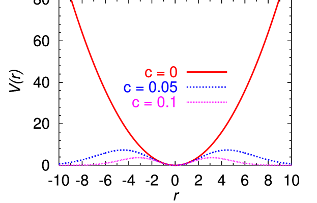
Figure 1: The scaled potential well $V(r)=r^{2}\exp(-cr^{2})$ for $c=0$, 0.05, and 0.1 (upper to lower curves).

We use the radially-symmetric time-dependent mean-field quantum-mechanical GP equation with attractive nonlinearity for the present study [12]. The time-dependent approach is useful to study the stability of the bound state under small perturbation. As we shall not be concerned with a particular experimental system, we write the GP equation in dimensionless variables. The GP equation for the Bose-Einstein condensate wave function $\psi({r};t)$ at position ${r}$ and time $t$ can be written in dimensionless form as [10]

$$\biggr{[} - i\frac{\partial}{\partial t}-{\frac{\partial^{2}}{\partial r^{2}}-\frac{D-1}{r}\frac{\partial}{\partial r}}+r^{2}e^{-cr^{2}}-g\left|{\psi({r};t)}\right|^{2}\biggr{]}\psi({r};t)=0,$$ (2.2)

where $-g$ is the attractive nonlinearity and $D=2,3,$ is the spatial dimension. In this paper we shall consider only attractive nonlinearity corresponding to positive $g$ values. Here length and time are expressed in units of $l$ and $(\omega/2)^{-1}$, respectively.

In 3D, in terms of number of atoms ${\cal N}$ and atomic scattering length $a$, the nonlinearity is given by $g=8\pi{\cal N}a/l.$ A scaled nonlinearity $n$ is often defined by $n=g/(8\pi)={\cal N}a/l.$ The normalization condition in (2.2) is $\int d^{D}{r}|\psi({r};t)|^{2}=1,$ with $d^{2}r=2\pi rdr$ and $d^{3}r=4\pi r^{2}dr$.

2.2 Axially-Symmetric Well

We consider the time-dependent GP equation in dimensionless variables for an axially-symmetric well. The GP equation for the Bose-Einstein condensate wave function $\psi({r},z;t)\equiv\phi({r},z;t)/r$ at radial position $r$, axial position $z$ and time $t$ can be written as [16]

$$\biggr{[} - i\frac{\partial}{\partial t}-{\frac{\partial^{2}}{\partial r^{2}}+\frac{1}{r}\frac{\partial}{\partial r}-\frac{\partial^{2}}{\partial z^{2}}}+(r^{2}+\lambda^{2}z^{2})e^{-c(r^{2}+\lambda^{2}z^{2})}$$ (2.3)

$$- \frac{1}{r^{2}}-8\pi n\left|\frac{\phi({r,z};t)}{r}\right|^{2}\biggr{]}\phi({r,z};t)=0,$$

with normalization

$$2\pi\int_{-\infty}^{\infty}dz\int_{0}^{\infty}rdr|\psi(r,z;t)|^{2}=1,$$ (2.4)

where $V(r,z)=(r^{2}+\lambda^{2}z^{2})e^{-c(r^{2}+\lambda^{2}z^{2})}$ is the axial trap. Here length and time are expressed in units of $l(\equiv\sqrt{\hbar/(m\omega)})$ and $(\omega/2)^{-1}$. respectively, with $\omega$ the radial trap frequency and $n={\cal N}a/l$ the scaled nonlinearity. In our calculation we shall set $\lambda=0$ so that the bound state develops solitonic transportation property along $z$ axis, and also take a finite $c$ so that the infinite radial trap is reduced to a shallow trap. Hence this model allows the study of bound states in 3D under the action of a weak radial trap alone where the binding comes mostly from the nonlinear interaction.

3 Variational Results

To understand how the bound states are formed in a radially-symmetric shallow well in 2D and 3D we employ a variational method with the following Gaussian wave function for the solution of (2.2) [16]

$$\psi(r,t)=A(t)\exp\left[-\frac{r^{2}}{2R^{2}(t)}+\frac{i}{2}{\beta(t)}r^{2}+i\alpha(t)\right],$$ (3.1)

where $A(t)$, $R(t)$, $\beta(t)$, and $\alpha(t)$ are the normalization, width, chirp, and phase of the soliton, respectively. In 3D $A(t)=[\pi^{3/4}R^{3/2}(t)]^{-1}$, and in 2D $A(t)=[\pi^{1/2}R(t)]^{-1}$. The Lagrangian density for generating (2.2) is [16, 17]

$${\cal L}(\psi) = \frac{i}{2}\left(\dot{\psi}\psi^{*}-\dot{\psi}^{*}\psi\right)-\left|\frac{\partial\psi}{\partial r}\right|^{2}-r^{2}e^{-cr^{2}}|\psi|^{2}+\frac{1}{2}g|\psi|^{4},$$ (3.2)

where the overhead dot represents time derivative. The trial wave function (3.1) is substituted in the Lagrangian density and the effective Lagrangian $L_{\mbox{eff}}$ is calculated by integrating the Lagrangian density: $L_{\mbox{eff}}=\int{\cal L}(\psi)d^{D}r.$ The Euler-Lagrange equations for this effective lagrangian are given by

$$\frac{d}{dt}\frac{\partial L_{\mbox{eff}}}{\partial\dot{\gamma}(t)}=\frac{\partial L_{\mbox{eff}}}{\partial\gamma(t)},$$ (3.3)

where $\gamma(t)$ stands for $R(t)$, $\beta(t)$, or $\alpha(t)$.

3.1 Radial symmetry in Three Dimensions

In 3D the effective Lagrangian is given by [17]

$$L_{\mbox{eff}} =\frac{\pi^{3/2}A^{2}(t)R^{3}(t)}{2}\biggr{[}-\frac{3}{2}\dot{\beta}(t)R^{2}(t)+\frac{1}{2\sqrt{2}}gA^{2}(t)$$ (3.4)

$$- 2\dot{\alpha}(t)-\frac{3}{R^{2}(t)}-3\beta^{2}(t)R^{2}(t)-\frac{3R^{2}(t)}{[1+cR^{2}(t)]^{5/2}}\biggr{]}.$$

The Euler-Lagrange equations for $\alpha(t)$, $A(t),\beta(t),$ and $R(t)$ are given, respectively, by

$$\pi^{3/2}A^{2}R^{3}=\mbox{constant}=1,$$ (3.5)

$$\dot{\beta}+\frac{4\dot{\alpha}}{3R^{2}}+\frac{2}{R^{4}}+2\beta^{2}+\frac{2}{(1+cR^{2})^{5/2}}=\frac{2gA^{2}}{3\sqrt{2}R^{2}},$$ (3.6)

$$\dot{R}=2R\beta,$$ (3.7)

$$5\dot{\beta}+\frac{4\dot{\alpha}}{R^{2}}+\frac{2}{R^{4}}+10\beta^{2}+\frac{10}{(1+cR^{2})^{7/2}}=\frac{gA^{2}}{\sqrt{2}R^{2}},$$ (3.8)

where the time dependence of the different observables is suppressed. Eliminating $\alpha$ between (3.6) and (3.8) one obtains

$$2\dot{\beta}=\frac{4}{R^{4}}-4\beta^{2}-\frac{gA^{2}}{\sqrt{2}R^{2}}-\frac{4-6cR^{2}}{(1+cR^{2})^{7/2}}.$$ (3.9)

From (3.7) and (3.9) we get the following second-order differential equation for the evolution of the width

$$\frac{d^{2}R}{dt^{2}} = \frac{4}{R^{3}}-\frac{g}{\sqrt{2\pi^{3}}}\frac{1}{R^{4}}-\frac{4R-6cR^{3}}{(1+cR^{2})^{7/2}}$$ (3.10)

$$= -\frac{d}{dR}\left[\frac{2}{R^{2}}-\frac{g}{3\sqrt{2\pi^{3}}}\frac{1}{R^{3}}+\frac{2R^{2}}{(1+cR^{2})^{5/2}}\right].$$ (3.11)

The quantity in the square brackets of (3.11) is the effective potential $U(R)$ of the equation of motion:

$$U(R)=\frac{2}{R^{2}}-\frac{8}{3\sqrt{2\pi}}\frac{n}{R^{3}}+\frac{2R^{2}}{(1+cR^{2})^{5/2}}.$$ (3.12)

Small oscillation around a stable configuration might be possible when there is a minimum in this effective potential.

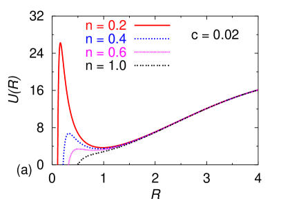
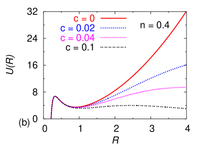
Figure 2: The effective potential $U(R)$ in 3D of (3.12) vs. $R$ in arbitrary units for (a) $c=0.02$ and $n\equiv g/(8\pi)=0.2,0.4,0.6,$ and $1.0$ (upper to lower curves) and for (a) $n=0.4$ and $c=0,0.02,0.04,$ and $0.1$ (upper to lower curves).

A study of the effective potential (3.12) as a function of parameters $n$ and $c$ reveals some interesting features. The small-$R$ part of $U(R)$ is insensitive to $c$ whereas, for small $c$, the long-$R$ part of $U(R)$ is insensitive to $n$. This is illustrated through the plot of $U(R)$ vs. $R$ for different $n$ and $c$ in figures 2 (a) and (b). The minimum of $U(R)$ for $R\approx 1$ representing a shallow effective well can allow a bound solution of the GP equation. For $c>0$, there cannot be a stable bound state in the linear problem where $g=n=0$. Although a minimum could appear in $U(R)$ in that case for a small $c$, the state becomes metastable and decays eventually by tunneling to infinity. This is possible as $U(R)\to 0$ as $R\to\infty$. The variational approach alone does not distinguish between a stable and a metastable state.

In figure 2 (a) we see that as the attractive nonlinearity $n$ is increased for a fixed $c$, one of the walls of the well is gradually lowered and for a sufficiently large $n$ this wall is completely absent and the condensate collapses into the infinitely deep well at the center. This happens for critical nonlinearity $n_{\mbox{crit}}\approx 0.6$ representing the onset of collapse. This value is to be compared with the accurate numerical value of 0.575 [12, 16] for the infinite harmonic potential with $c=0$. We also find in figure 2 (b) that, for a fixed $n$, as $c$ is increased from 0, the shallow well lasts up to a finite value of $c$ beyond which there is no well for the formation of a bound state $-$ stable or metastable. The simple variational study qualitatively describes the formation of an attractive BEC in a shallow finite potential. Also, in such case of critical equilibrium the variational treatment usually over-binds the system and does not yield reliable results, for which we consider the direct numerical treatment in the next section.

3.2 Radial symmetry in Two Dimensions

In 2D the effective Lagrangian is given by [17]

$$L_{\mbox{eff}} ={\pi A^{2}(t)R^{2}(t)}\biggr{[}-\frac{1}{2}\dot{\beta}(t)R^{2}(t)+\frac{1}{4}gA^{2}(t)-\dot{\alpha}(t)$$ (3.13)

$$- \frac{1}{R^{2}(t)}-\beta^{2}(t)R^{2}(t)-\frac{R^{2}(t)}{[1+cR^{2}(t)]^{2}}\biggr{]}.$$

As in the three-dimensional case one can write the the coupled Euler-Lagrange equations for $\alpha(t)$, $A(t),\beta(t),$ and $R(t)$. After some algebra one can eliminate the variables $\alpha(t)$, $A(t),$ and $\beta(t)$ from these equations and

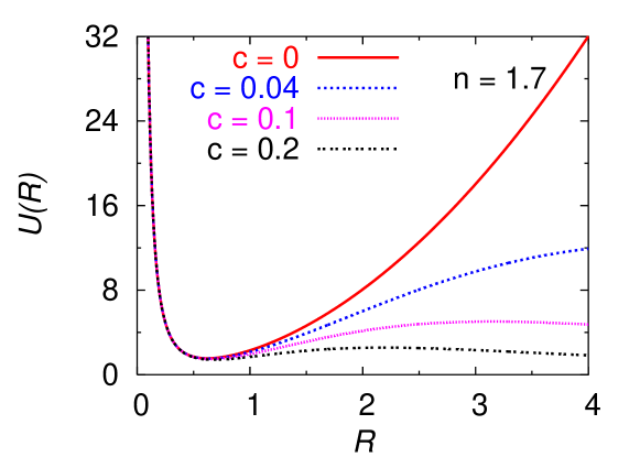
Figure 3: The effective potential $U(R)$ in 2D of (3.16) vs. $R$ in arbitrary units for $n\equiv g/(2\pi)=1.7$ and $c=0,0.04,0.1,$ and $0.2$ (upper to lower curves).

obtain the following second-order differential equation for the evolution of the width $R$

$$\frac{d^{2}R}{dt^{2}} = \frac{4}{R^{3}}-\frac{g}{\pi}\frac{1}{R^{3}}-\frac{4(R-cR^{3})}{(1+cR^{2})^{3}}$$ (3.14)

$$= -\frac{d}{dR}\left[\frac{2(1-g/4\pi)}{R^{2}}+\frac{2R^{2}}{(1+cR^{2})^{2}}\right].$$ (3.15)

In this case the effective potential $U(R)$ for the evolution of the width is given by

$$U(R)=\frac{2-n}{R^{2}}+\frac{2R^{2}}{(1+cR^{2})^{2}},$$ (3.16)

where $n=g/(2\pi)$ in 2D.

The study in 2D reveals similar qualitative features as in 3D. From (3.16) we see trivially that the onset of collapse is given in this case by $n=2$. This has to be compared with the numerical value $n\approx 1.85$ [18, 19, 20] obtained by solving the GP equation in 2D with $c=0$. For $n>2$, $U(R)$ does not have a barrier for small $R$ and the collapse cannot be avoided. There is no such simple analytic condition of collapse in 3D where it can be numerically obtained from (3.12).

In figure 3 we plot $U(R)$ for different $c$ values for $n=1.7$. As in 3D we find that with an increase of $c$ the outer wall of the well is gradually reduced and for a large enough $c$ this wall is completely removed and no bound state is possible. Again, although the simple variational study reveals these qualitative features, it is not so useful for a quantitative study in this region of critical stability. Also, it cannot distinguish between a stable and a metastable state.

4 Numerical Results

We solve the GP equations (2.2) and (2.3) for shallow potential wells in 2D and 3D numerically using the split-step time-iteration method employing the Crank-Nicholson discretization scheme described recently [13, 21]. In the radially-symmetric case the time iteration is started with the known oscillator solution of these equations with $n=c=0$. In the axially-symmetric case in the initial configuration a small finite axial trap parameter $\lambda$ is employed. Then in the course of time iteration the attractive nonlinearity $n$ and the parameter $c$ of the potential are switched on slowly. In the axially-symmetric case the parameter $\lambda$ is gradually turned off during time iteration. If stabilization could be obtained for the chosen parameters one already obtains the required bound state in the shallow trap.

Stable bound states are indeed found in all cases for various ranges of parameters: $c$ and $n$. Some plausible properties of the bound states are found. Stable bound states are only formed for $c$ less than a critical value. For larger $c$, from the wisdom obtained in variational calculation, the effective potential $U(R)$ does not have a minimum and there cannot be any bound state. For a fixed $c$, bound states are found for $\bar{n}<n<n_{\mbox{crit}}$. For $n>n_{\mbox{crit}}$ the system is very attractive and collapses. For $n<\bar{n}$, the system is very weakly attractive and expands to infinity. The quantum state is then metastable. The numerical values of $\bar{n}$ and $n_{\mbox{crit}}$ are different in 2D and 3D. As $c$ is reduced to zero, both $\bar{n}$ and $n_{\mbox{crit}}$ decreases. Finally, at $c=0$, $n_{\mbox{crit}}$ reduces to the critical nonlinearity for collapse in the full harmonic trap [12, 16] and $\bar{n}$ reduces to zero. This is consistent with the fact that in the full harmonic trap, one can have a stable bound state for all attractive nonlinearities smaller than a critical value. Also, for $c>0$ the critical nonlinearity for collapse $n_{\mbox{crit}}$ is larger than the critical nonlinearity for the full harmonic trap.

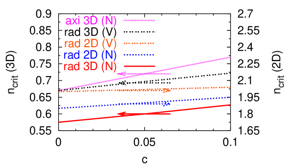
Figure 4: Results of variational (V) and numerical (N) calculations for critical nonlinearity $n_{\mbox{crit}}$ in radially-symmetric 3D, axially-symmetric 3D, and radially-symmetric 2D for different values of the parameter $c$.

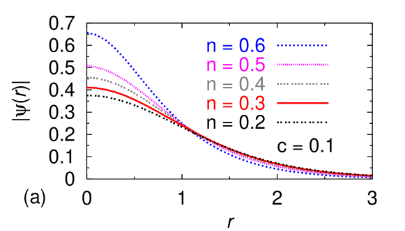
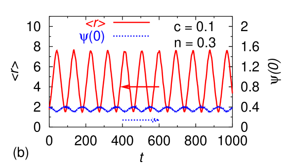
Figure 5: (a) Stable bound-state wave function $|\psi(r)|$ of the radially-symmetric GP equation (2.2) in 3D with $c=0.1$ and scaled nonlinearity $n\equiv g/(8\pi)=0.6,0.5,0.4,0.3,$ and 0.1 (upper to lower curves); (b) $|\psi(r=0)|$ (lower curve) and rms radius $\langle r\rangle$ (upper curve) of the bound-state wave function for $c=0.1$ and $n=0.3$ executing breathing oscillation initiated by multiplying the shallow trapping potential suddenly at $t=0$ by 0.95.

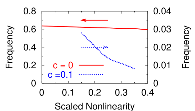
Figure 6: Frequency of breathing oscillation vs. scaled nonlinearity $n$ for $c=0$ and 0.1 in the radially symmetric 3D case. Note the different scales used for $c=0$ and 0.1.

4.1 Radial Symmetry in Three Dimensions

First we present the numerical results in 3D. For $c=0$, $n={\cal N}a/l=0.575$ is the critical nonlinearity for collapse [12]. For $c=0.1$, the confining shallow potential is weaker and the critical nonlinearity of collapse is larger and a stable bound state could be formed for $n=0.6$. As the nonlinearity $n$ is increased, the system becomes more attractive and the wave function develops a central peaking. In figure 4 we plot the variational and numerical results for the critical nonlinearity for collapse for different values of $c$ in 3D and 2D. This plot illustrates how the critical nonlinearity increases with $c$ for radial and axial (discussed in section 4.3) symmetry in 3D and radial symmetry in 2D (discussed in section 4.2). The variational results are always larger than the numerical ones.

Recently, there has been another study of BEC bound states in shallow traps (2.1) by Moiseyev et al [15]. They conclude that there cannot be stable bound states in 3D in shallow traps (2.1). We do not know the reason for this disagreement. As $c\to 0$, the potential (2.1) tends to an infinite harmonic trap. For large $c$ the potential becomes very shallow and it is reasonable that these bound states should disappear. We find it hard to believe that these states should not exist for a small value of $c$ when the potential tends to a pure harmonic one. We iterated the GP equation for more than 10 000 time units corresponding to a million time iterations and the bound-state wave function remained unchanged demonstrating its stability.

In figure 5 (a) we plot the wave function for the bound state of the GP equation (2.2) for $c=0.1$ and different $n\equiv g/(8\pi)={\cal N}a/l$. To study the stability of the bound state under small perturbation, we study breathing oscillation in the bound state by suddenly changing the strength of the shallow trapping potential from 1 to 0.95. The system executes harmonic oscillations around a stable configuration illustrated in figure 5 (b), where we plot the root-mean-square (rms) radius $\langle r\rangle$ and $\psi(0)$ vs. time for $c=0.1$ and $n=0.3$. The prolonged stable oscillation of these states for an interval of time of more than 1000 units assures us of their stable, opposed to metastable, nature.

From figure 1 we see that for $c=0.1$ the shallow trapping potential is highly reduced compared to the full harmonic potential. In the GP equation (2.2), in this case the binding is provided mostly by the nonlinear interaction. Hence the oscillation depicted in figure 5 (b) is highly nonlinear in nature. In the $c=0$ case we studied in detail this breathing oscillation and the frequency $\nu$ of the breathing oscillation was roughly double the frequency of the trapping potential $\omega$ (= 2 in present units) and independent of nonlinearity $n$: $\nu\approx 2\times\omega/2\pi=2/\pi\approx 0.636$ [13]. However, the present frequency of highly nonlinear oscillation in figure 5 (b) is approximately 0.011 $-$ completely different from the $c=0$ case. The breathing frequency is found to be sensitive to the nonlinearity in the GP equation for $c=0.1$. To illustrate this we plot in figure 6 the variation in breathing frequency with nonlinearity for $c=0$ and $c=0.1$. The frequencies for $c=0$ and $c=0.1$ are distinct: the frequencies for the shallow well with $c=0.1$ are sensitive to the nonlinearity. For this small variation of nonlinearity the frequencies for the infinite well are practically independent of nonlinearity. However, the frequencies for the infinite well will gain a weak dependence on nonlinearity for large repulsive interactions (not discussed here). As nonlinearity $n$ is reduced below 0.15 for $c=0.1$, first the breathing oscillation enters a chaotic regime with no well defined frequency and with further reduction in $n$ the bound state becomes metastable. Also, as nonlinearity $n$ is increased beyond 0.35 for $c=0.1$, the oscillation becomes irregular and we did not study it in detail.

The highly nonlinear breathing oscillation of the condensate discussed above is not only of theoretical interest but could be studied in the laboratory with present knowhow. The infinite harmonic trap can slowly be reduced to generate a shallow potential after the formation of an attractive condensate and the highly nonlinear breathing oscillation could be studied. A careful study of this oscillation will reveal interesting features of this dynamics and could be used to compare the experimental results with mean-field predictions.

4.2 Radial Symmetry in Two Dimensions

Now we present the numerical results in 2D. In figure 7 we plot the wave function for the solution of the GP equation (2.2) for $c=0.1$ and different values of nonlinearity $n=g/(2\pi)$. For $c=0$ the critical nonlinearity for collapse is $n\approx 1.85$ [18, 19, 20]. For $c=0.1$, one can have a larger value for the critical nonlinearity. A variation of critical nonlinearity in this case is shown in figure 4. With the increase of the nonlinearity $n$, the nonlinear atomic attraction increases and the condensate is confined to a smaller region in space. Consequently, in figure 7 the wave function has a stronger central peaking for larger nonlinearity as in 3D. The critical nonlinearity for collapse calculated by Moiseyev et al [15] ($\sim 1.72$) is typically smaller than our estimate ($>1.85$). [Note that the values reported by them ($\sim 0.86$) differ from the present values by a factor of 2 because of a slightly different nonlinear equation used by them.] Again the reason for this disagreement is not clear.

We also noted the highly nonlinear breathing oscillation in this case for $c=0.1$ initiated by a sudden change in the strength of the harmonic interaction. Unlike in the $c=0$ case, where the frequency of breathing oscillation is virtually independent of small changes in nonlinearity, in this case the frequency of breathing oscillation is quite sensitive to the nonlinearity in the GP equation. However, a complete and comprehensive analysis of this nonlinear breathing oscillation is beyond the scope of this paper and will be one of future interest.

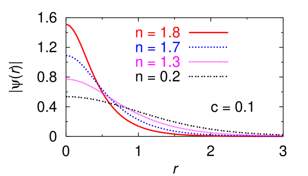
Figure 7: Stable bound-state wave function $|\psi(r)|$ of the radially-symmetric GP equation (2.2) in 2D with $c=0.1$ and nonlinearity $n\equiv g/(2\pi)=1.8,1.7,1.3,$ and 0.2 (upper to lower curves).

4.3 Axial Symmetry in Three Dimensions

Finally, we consider the case of an axially-symmetric stable bound state in 3D. This is of interest as most of the experimental condensates possess axial symmetry. We consider the numerical solution of the time-dependent GP equation (2.3) for our purpose, with $\lambda=0$ and $c=0.1$. This case corresponds to the $z$-independent scaled potential $V(r,z)=r^{2}\exp(-0.1r^{2})$. This means that the bound state is free to move along the axial $z$ axis and bound radially by the above weak potential. The critical nonlinearity for collapse in this case for different $c$ is plotted in figure 4. The profile of the bound states in this case is shown in figures 8 (a) $-$ (d) where we plot the stationary wave function $|\psi(r,z)|$ of (2.3) for nonlinearities $n=0.1,0.4,0.6$ and 0.7, respectively. As the axial trap is removed the condensate is very long in the $z$ direction and possesses a small radius. In figures 8 we see that the condensate has the shape of a cigar about 50 units long with a radius of 2 units. As the nonlinearity is increased from $n=0.1$ to 0.7 in figures 8, the condensate collapses towards the center resulting in a high central peaking. This aspect is similar to solitons in 1D where a similar peaking is observed with the increase of nonlinearity. However, there is no collapse in 1D. In the radially symmetric case $\lambda=1$ and $c=0$, the BEC could be formed for nonlinearity $n$ less than a critical value $n_{\mbox{crit}}=0.575$ [12, 16]. For the usual three-dimensional bound state $c=\lambda=0$, $n_{\mbox{crit}}=0.67$ [5, 7]. In the present case $c=0.1$ and $\lambda=0$, $n_{\mbox{crit}}$ is greater than 0.7. In all cases, for $n>n_{\mbox{crit}}$, the bound state becomes highly attractive and collapses, so that no stable bound state could be formed. The reduction of $\lambda$ from 1 to 0 or the increase in $c$ from 0 to 0.1 in these cases denotes a weakening of the confining trap. Consequently, the condensate can occupy a larger region of space and accommodate a larger number of particles (or nonlinearity) before collapsing, corresponding to an increase in $n_{\mbox{crit}}$. In this case also one could have breathing oscillation as in the radially-symmetric case. This oscillation will be more complicated, specially for the interesting case of $c=0.1$, involving two degrees of freedom and its study is not appropriate for this paper.

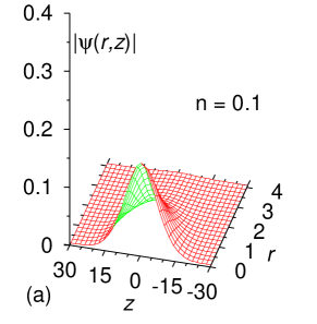
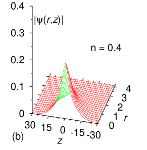
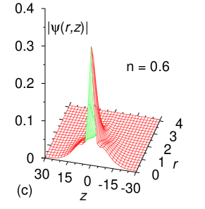
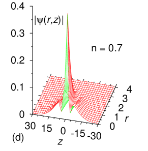
Figure 8: Stable bound-state wave function $|\psi(r,z)|$ of the axially-symmetric GP equation (2.3) in 3D with $c=0.1$ and $\lambda=0$ and nonlinearity $n=$ (a) 0.1, (b) 0.4, (c) 0.6 and (d) 0.7. The $z$-independent trapping potential is $V(r,z)=r^{2}\exp(-0.1r^{2})$.

5 Discussion and Conclusion

The study of the dynamics of one-dimensional solitons is of great interest in different areas of science and mathematics because of its intrinsic nonlinear nature. In the three-dimensional world, one-dimensional systems can only be achieved in some approximation. Also, it is difficult to find a true three-dimensional soliton in nature bound only under the action of a nonlinear interaction. BECs with attractive atoms are very appropriate for the study of nonlinear dynamics as the GP equation describing the BEC dynamics possesses a cubic nonlinear (Kerr) interaction which is identical with the sole interaction term in the one-dimensional NLS (1.1). However, unlike in one-dimensional solitons, in 2D and 3D an infinite confining potential has to be included in the GP equation for the formation of a stable BEC [12]. To have a greater similarity with freely moving one-dimensional solitons, later it was shown that stable three-dimensional bound states moving in the axial direction like a soliton could be formed after removing the axial trap in an axially-symmetric configuration maintaining an infinite radial trap [5]. However, the strong infinite radial trap, and not the weaker cubic nonlinear interaction, controls the essential dynamics of these objects. In this paper we showed that similar objects could be formed even when the infinite radial trap is reduced to an exponentially-screened harmonic potential. Under the action of such a weak radial trap, the cubic nonlinear interaction plays a major role on dynamics.

To establish the present suggestion we solved the GP equation numerically to find the bound states in the radially-symmetric potential $V(r)=r^{2}\exp(-0.1r^{2})$ in 2D and 3D. We studied in some detail the breathing oscillation of such a bound state in 3D. The frequency of this oscillation is found to be sensitive to the nonlinearity of the problem. In the infinite harmonic potential $V(r)=r^{2}$, the frequency of breathing oscillation is found to be weakly dependent on the nonlinearity of the problem (at least for small nonlinearities) and determined mostly by the frequency of the trapping potential. We finally demonstrate numerically the existence of these bound states in the $z$-independent axially-symmetric potential $V(r,z)=r^{2}\exp(-0.1r^{2})$. Such axially free and radially bound states of BEC under the action of a weak trap can be formed and studied in the laboratory.

It is appropriate to make a prediction of the height of the trap (2.1) to be used in experimental set ups for the value of the parameter $c=0.1$. The GP equation we used is strictly valid at 0 K [12]. For a trap frequency $\omega\sim 2\pi\times 100$ Hz, $\hbar\omega\sim 5$ nK. In that case from figure 1 we find that the height of the reduced trap (2.1) is around 20 nK for a condensate at 0 K, as the scaled potential is expressed in units of $\hbar\omega$. However, the condensates in the laboratory are observed often at $50-100$ nK, and the height of the reduced trap in the laboratory should be higher than this value. We could not predict the minimum height for forming the BEC bound states in different cases. However, a good conservative estimate should be $200-400$ nK, the correct value can only be obtained in actual experiment. The quantitative results about critical nonlinearity for the formation of BEC states in figure 4 and about the frequency of oscillation of the BEC in figure 6 could be verified in the laboratory and compared with theoretical predictions.

References

References

- [1] Hasegawa A and Tappert F 1973 App. Phys. Lett. 23 171 Hasegawa A and Tappert F 1973 App. Phys. Lett. 23 142 Zakharov V E and Shabat A B 1972 Sov. Phys. JETP 34 62 Zakharov V E and Shabat A B 1973 Sov. Phys. JETP 37 823
- [2] Kivshar Y S and Agrawal G P 2003 Optical Solitons - From Fibers to Photonic Crystals (San Diego, Academic Press)
- [3] Denschlag J, Simsarian J E, Feder D L, Clark C W, Collins L A, Cubizolles J, Deng L, Hagley E W, Helmerson K, Reinhardt W P, Rolston S L, Schneider B I and Phillips W D 2000 Science 287 97
- [4] Strecker K E, Partridge G B, Truscott A G and Hulet R G 2002 Nature 417 150 Khaykovich L, Schreck F, Ferrari G, Bourdel T, Cubizolles J, Carr L D, Castin Y and Salomon C 2002 Science 296 1290
- [5] Pérez-García V M, Michinel H and Herrero H 1998 Phys. Rev. A 57 3837
- [6] Al Khawaja U, Stoof H T C, Hulet R G, Strecker K E and Partridge G B 2002 Phys. Rev. Lett.89 200404
- [7] Adhikari S K 2003 New J. Phys.5 137 Adhikari S K 2004 Few-Body Syst. 34 197
- [8] Kivshar Y S, Alexander T J and Turitsyn S K 2001 Phys. Lett.A 278 225
- [9] Saito H and Ueda M 2003 Phys. Rev. Lett.90 040403 Abdullaev F K, Caputo J G, Kraenkel R A and Malomed B A 2003 Phys. Rev.A 67 013605 Adhikari S K 2004 Phys. Rev.E 70 036608
- [10] Adhikari S K 2004 Phys. Rev. A 69 063613
- [11] Abdullaev F K, Baizakov B B and Salerno M 2003 Phys. Rev.E 68 066605 Adhikari S K 2005 Phys. Rev.E 71 0166xx
- [12] Dalfovo F, Giorgini S, Pitaevskii L P and Stringari S 1999 Rev. Mod. Phys. 71 463
- [13] Adhikari S K and Muruganandam P 2002 J. Phys. B: At. Mol. Opt. Phys. 35 2831
- [14] Hai W, Lee C and Chong G 2004 Phys. Rev.A 70 053621
- [15] Moiseyev N, Carr L D, Malomed B A and Band Y B 2004 J. Phys. B: At. Mol. Opt. Phys. 37 L193
- [16] Adhikari S K 2002 Phys. Rev. E 65 016703
- [17] Abdullaev F K, Caputo J G, Kraenkel R A and Malomed B A 2003 Phys. Rev. A 67 013605
- [18] Adhikari S K 2000 Phys. Lett. A 265 91 Adhikari S K 2000 Phys. Rev. E 62 2937
- [19] Gammal A, Frederico T, Tomio L and Abdullaev F K Phys. Lett. A 267 305
- [20] Dudarev A M, Diener R B and Niu Q 2004 J. Opt. B: Quantum Semiclass. Opt.6 S231
- [21] Muruganandam P and Adhikari S K 2003 J. Phys. B: At. Mol. Opt. Phys. 36 2501