Real-space renormalization-group approach
to the integer quantum Hall effect

Abstract

We review recent results based on an application of the real-space renormalization group (RG) approach to a network model for the integer quantum Hall (QH) transition. We demonstrate that this RG approach reproduces the critical distribution of the power transmission coefficients, i.e., two-terminal conductances, $P_{\rm c}(G)$, with very high accuracy. The RG flow of $P(G)$ at energies away from the transition yields a value of the critical exponent $\nu$ that agrees with most accurate large-size lattice simulations. A description of how to obtain other relevant transport coefficients such as $R_{\rm L}$ and $R_{\rm H}$ is given. From the non-trivial fixed point of the RG flow we extract the critical level-spacing distribution (LSD). This distribution is close, but distinctively different from the earlier large-scale simulations. We find that the LSD obeys scaling behavior around the QH transition with $\nu=2.37\pm 0.02$. Away from the transition it crosses over towards the Poisson distribution. We next investigate the plateau-to-insulator transition at strong magnetic field. For a fully quantum coherent situation, we find a quantized Hall insulator with $R_{\rm H}\approx h/e^{2}$ up to $R_{\rm L}\sim 20h/e^{2}$ when interpreting the results in terms of most probable value of the distribution function $P(R_{\rm H})$. Upon further increasing $R_{\rm L}\rightarrow\infty$, the Hall insulator with diverging Hall resistance $R_{\rm H}\propto R_{\rm L}^{\kappa}$ is seen. The crossover between these two regimes depends on the precise nature of the averaging procedure for the distributions $P(R_{\rm L})$ and $P(R_{\rm H})$. We also study the effect of long-ranged inhomogeneities on the critical properties of the QH transition. Inhomogeneities are modeled by a smooth random potential with a correlator which falls off with distance as a power law $r^{-\alpha}$. Similar to the classical percolation, we observe an enhancement of $\nu$ with decreasing $\alpha$. These results exemplify the surprising fact that a small RG unit, containing only five nodes, accurately captures most of the correlations responsible for the localization-delocalization transition.

1 Introduction

Measuring the resistance of a two-dimensional (2D) electron gas at very low temperature and subject to a strong perpendicular magnetic field $B$ reveals a striking macroscopic quantum phenomenon [1]: the Hall resistance $R_{\rm H}$ shows very precise plateaus at $(1/N)h/e^{2}$ where $N$ is an integer number. In the same region the vanishing longitudinal resistance $R_{\rm L}$ indicates a dissipationless flow of current. Quantization can also be observed at fractional values of $N$ [2], which leads to the distinction between the fractional and the integer quantum Hall (QH) effect. Despite the similarities regarding the experimental observations the theoretical description of both effects differs considerably. The integer QH effect can be explained reasonably well within a non-interacting electron picture, while interactions play a fundamental role in the fractional QH effect [3, 4].

The integer QH effect can be rationalized at a phenomenological level as a series of localization-delocalization transitions [5]. For non-interacting electrons, the density of states consists of distinct Landau bands. These are broadened by the intrinsic disorder of the QH samples. Each such band contains localized states in the tails and extended states in the center of the band. As the Fermi energy passes through the extended states, the Hall resistance $R_{\rm H}$ rises to the next plateau and the longitudinal resistance $R_{\rm L}$ is non-vanishing. In the range between the bands and for the localized states the Hall resistance remains fixed at the plateau value as shown in Fig. 1.

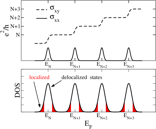
Figure 1: Schematic behavior of longitudinal ($\sigma_{xx}$) and Hall ($\sigma_{xy}$) conductivities as well as the density-of-states (DOS) for the integer QH effect. $E_{\rm F}$ denotes the Fermi energy and the energy of the Landau levels is $E=\hbar\omega_{\rm c}(N-1/2)$, $N=1,2,\ldots$; $\omega_{\rm c}=eB/m$ the cyclotron frequency. The width of the region of extended states at the band centers of the disorder-broadened Landau levels is finite due to finite temperatures and finite system sizes.

Several theoretical approaches have been proposed to explain the sequence of integer QH transitions in more detail [5, 3, 6, 7, 8, 9, 10, 4]. For example, it has been established that the QH transition is a second-order phase transition [11] where a power-law divergence of characteristic length scales is observed. The divergence, e.g. of the localization length $\lambda$ of the wave functions, $\lambda\propto\epsilon^{-\nu}$, where $\epsilon$ corresponds to the distance from the transition, can be quantified by the exponent $\nu$. Its value is a universal quantity, independent from microscopic details of electron motion, disorder realization and even the chosen material.

The Chalker-Coddington (CC) model is a convenient representation of the QH situation in the fully quantum coherent regime at low temperature and strong magnetic field [12]. The model describes a single Landau band and thus contains only one QH transition. Electrons are treated semiclassically as non-interacting particles moving in a smoothly varying 2D disorder potential under a strong perpendicular magnetic field. The percolation of the electron through the sample is then given by motion along equipotentials interrupted by scattering events at saddle points (SPs) of the potential. For theoretical investigations, equipotentials and SPs are mapped on links and nodes of a 2D network, respectively, and large networks have to be studied in order to reduce finite-size effects [13, 12, 14, 15, 16, 17].

In the present review, we concentrate on an alternative approach to the CC model. Namely, we shall introduce a real-space renormalization-group (RG) approach [18, 19], based on mapping a characteristic part of the CC network — the RG unit — consisting of several SPs onto a single super-SP residing in a new CC-super network. This approach is motivated by the success of RG techniques in statistical physics and particularly the study of phase transitions [20, 21]. Common to both real-space[22] and field-theoretical [23] RGs is the elimination of irrelevant (either short-range or short-period) degrees of freedom. Afterwards the original phase volume is restored by a scale transformation. The system has now the same structure as the original but the parameters, e.g. coupling constants, are renormalized. During the iteration of the above RG steps the parameters approach their fixed point (FP) values and an analysis of this convergence allows one to derive the critical properties of the transition. Large effective system sizes can be achieved in this way for the CC model. This advantage is counterbalanced by the approximate description of the network due to the limited size of the RG unit.

The RG procedure provides a natural route to studying the complete distribution functions of the 2D resistivities defined via

$${\bf E}=\left(\begin{array}[]{cc}\rho_{xx}&\rho_{xy}\\ -\rho_{xy}&\rho_{xx}\\ \end{array}\right){\bf j},$$ (1)

where $\rho_{xx}$ is called longitudinal and $\rho_{xy}$ Hall resistivity. The conductivity tensor is defined as the inverse of the resistivity tensor which yields

$$\sigma_{xx}=\sigma_{yy}=\frac{\rho_{xx}}{\rho_{xx}^{2}+\rho_{xy}^{2}}\quad\mbox{and}\quad\sigma_{xy}=-\sigma_{yx}=-\frac{\rho_{xy}}{\rho_{xx}^{2}+\rho_{xy}^{2}}.$$ (2)

We emphasize that in 2D resistances (conductances) and resistivities (conductivities) are related by a simple, dimensionless geometrical factor.

As a first application of the real-space RG approach to the CC model, we study the distribution functions $P$ of two-point conductance $G$ and the resistances $R_{\rm L}$ and $R_{\rm H}$. From these, we compute the value of the critical exponent $\nu$. Furthermore, closing the incoming and outgoing links of the RG unit and thus quantizing the allowed energies, we can make contact with previous studies of energy level statistics. A suitable scaling ansatz again allows the independent estimation of $\nu$. These results are in good agreement with previous studies and validate the present RG approach.

A further application is concerned with the possible existence of the quantized Hall insulator. While it is established that plateau-plateau and insulator-plateau transitions exhibit the same critical behavior [24, 25, 26, 27, 28, 29, 30, 31, 32, 33, 34] the value of the Hall resistance $R_{\rm H}$ in this insulating phase is still rather controversial [35]. Various experiments have found that $R_{\rm H}$ remains very close to its quantized value $h/e^{2}$ even deep in the insulating regime when already $R_{\rm L}\gg h/e^{2}$ [25, 26, 36, 27, 28]. This scenario has been dubbed the quantized Hall insulator. On the other hand, theoretical predictions based on quantum coherent models show that a diverging $R_{\rm H}$ should be expected [37, 38]. Extending the RG approach to the calculation of suitable means for $R_{\rm H}$ and $R_{\rm L}$ we show that the RG approach can in fact reconcile these findings by establishing that the most-probable value of $R_{\rm H}$ remains rather close to $h/e^{2}$ even for large $R_{\rm L}$, but then diverges with the predicted power-law for $R_{\rm L}>20h/e^{2}$.

Last, the RG approach is also ideally placed to study the changes of the critical properties due to truly long-ranged, so-called macroscopic inhomogeneities. Close to the transition the localization length $\xi$ becomes sufficiently large. Then the long-ranged disorder can affect the character of the divergence of $\xi$. We note that in previous considerations inhomogeneities were incorporated into the theory through a spatial variation of the local resistivity [40, 41, 42, 43, 44], i.e., “inhomogeneously incoherent”. Our present approach is able to retain the full quantum coherence.

The results of this study are presented as follows. The main tool of this work, the RG approach to the CC model, is content of section 2. Results for resistance and conductance distributions, the level spacing statistics and the associated estimates of the critical exponent are reviewed in section 3. The extension of the RG approach for the QH insulator and for macroscopic inhomogeneities are presented in section 4. We conclude in section 5.

2 The quantum RG approach to the CC model

2.1 The Chalker-Coddington network model

The CC network model [12] uses a semi-classical approach to model the integer QH transition and is one of the main “tools” for the quantitative study of the QH transition [45, 46, 47, 48, 15, 49, 50, 51, 16, 17, 52, 53]. It is based on an extension of the high-field model [54]. In order to include the previously mentioned localization-delocalization scenario the classical high-field model relies on two basic prerequisites. First, the 2D sample is penetrated by a very strong perpendicular magnetic field and second the electrons are non-interacting and move in a smoothly varying 2D potential energy landscape $V({\bf r})$ illustrated in Fig. 2.

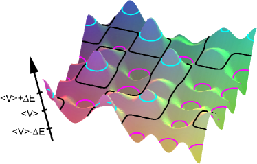
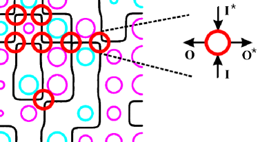
Figure 2: Left: Illustration of a weakly varying random potential $V$ with equipotential lines at $\langle V\rangle$ and $\langle V\rangle\pm\Delta E$ which allows to separate the electron motion (black orbit) in a strong magnetic field $B$ into cyclotron motion and motion of the guiding center along equipotentials. Right: From these equipotentials at $E=\langle V\rangle$, $\langle V\rangle\pm\Delta E$ SPs of the potential can be identified. A single SP acts as a scatterer connecting two incoming with two outgoing channels.

As a result the magnetic field $B$ forces an electron onto a cyclotron motion with radius $l_{\rm B}$ much smaller than the potential fluctuations. Thus the electron motion can be separated into cyclotron motion and a motion of the guiding center along equipotentials of the energy landscape [54]. The cyclotron motion leads to the required quantization into discrete Landau levels whereas its influence on the electron motion in the potential can be neglected. Besides the fundamental assumption about the difference of length scales the model therefore contains no further dependence on $B$. The quantum effects of the electron transport through the sample are only determined by the height of the SPs in the potential energy landscape. This picture is related to a classical bond percolation problem on a square lattice [55] when mapping SPs onto bonds. A bond is connecting only when the potential of the corresponding SP equals the potential energy $\varepsilon$ of the electron. From percolation theory [55] follows that an infinite system is conducting only at a single $\varepsilon=\langle V\rangle$. Consequently, the high-field model describes only a single QH transition. It provides a qualitative understanding of the existence of an localization-delocalization transition and thus the quantized plateaus in the conductivity $\sigma_{xy}$ observed in the integer QH effect [6]. However, because of its purely classical assumptions the model is unable to exactly reproduce the critical properties of the transition found in experiments, i.e., the divergence of the correlation length at the transition with an exponent of $\nu\approx 2.3$ [56]. Instead, it predicts $\nu=4/3$, the value appropriate for classical percolation.

The CC network model improved the high-field model by introducing quantum corrections [12], namely tunneling and interference. Tunneling occurs, in a semi-classical view, when electron orbits come so close to each other that the cyclotron orbits overlap. From Fig. 2 one can conclude that this happens at the SPs, which now act as quantum scatterers described by a unitary scattering matrix $S$

$$\left(\begin{array}[]{c}O\\ O^{*}\end{array}\right)=S\left(\begin{array}[]{c}I\\ I^{*}\end{array}\right)=\left(\begin{array}[]{cc}t&r\\ -r&t\end{array}\right)\left(\begin{array}[]{c}I\\ I^{*}\end{array}\right)$$ (3)

which connects two incoming with two outgoing channels. Assuming a symmetric potential at the SP the scattering rates are given by a pair of a complex transmission and a reflection coefficient $t$ and $r$, respectively. From the required unitarity of $S$ it follows that $|t|^{2}+|r|^{2}=1$. Obviously, $t$ and $r$ depend on the potential energy of the SP. It was shown [19] that $t$ and $r$ can be parametrized by

$$t=\left(\frac{1}{e^{z}+1}\right)^{\frac{1}{2}}\quad{\rm and}\quad r=\left(\frac{1}{e^{-z}+1}\right)^{\frac{1}{2}}$$ (4)

where $z$ corresponds to a dimensionless energy difference between SP potential and electron energy $\varepsilon$. Without restricting the generality $\langle V\rangle=0$ is assumed in the following. In case of $\varepsilon=0$ the value of $z$ then coincides with the dimensionless SP height. Similar to bond percolation now a network of SPs can be constructed. The SPs are mapped onto nodes and the equipotentials correspond to links. While moving along an equipotential an electron accumulates a random phase $\Phi$ which reflects the randomness of the potential. The corresponding phase factor $e^{i\Phi}$ can be included in the matrix $S$ [57] or taken into account by additional diagonal matrices on each link [19].

As in the high-field model this quantum percolation model describes only a single QH transition with exactly one extended state in the middle of the Landau band at $\varepsilon=0$ . The critical properties at the transition, especially the value of the exponent $\nu\approx 2.4\pm 0.2$ [16], agree with experiments [56, 34] as well as with results of other theoretical approaches [58, 59]. For numerical investigations of the CC model, one constructs a regular 2D lattice out of the SPs. Then the 2D plane is cut into 1D slices with the associated scattering matrices transformed into a transfer matrix. The conductivity may be calculated by transversing perpendicular to the slices along the sample by transfer matrix multiplications [16] according to the Landauer-Büttiker approach [60]. The spatial extension of the 2D plane is limited by the computational effort although an additional disorder averaging over many samples is not necessary for quasi-1D samples [16].

The CC model is a strong-magnetic-field (chiral) limit of a general network model, first introduced by Shapiro [61] and later utilized for the study of localization-delocalization transitions within different universality classes[62, 63, 64, 65, 66, 67]. In addition to the QH transition, the CC model applies to a much broader class of critical phenomena since the correspondence between the CC model and thermodynamic, field-theory and Dirac-fermions models [68, 69, 70, 71, 72, 73, 74, 75, 76] was demonstrated.

2.2 Derivation of the basic RG equation for transmission amplitudes

The real-space RG approach [18, 19] can be applied to the CC network analogously to the case of 2D bond percolation [77, 78, 79]. An RG unit is constructed containing several SPs from a CC network. For these SPs the RG transformation has to relate their $S$ matrices with the $S$ matrix of the super-SP. The RG unit used here is extracted from a CC network on a regular 2D square lattice. The super-SP consists of five original SPs connected according to Fig. 3. Circles correspond to SPs and lines to links in the network. Using this intuitive picture one can identify the loss of connectivity in comparison with the original CC network, namely, the four edge nodes within a $3\times 3$ SP pattern are fully neglected as are their outer bonds. Thus the super-SP has the same number of incoming and outgoing channels as an original SP. In analogy to bond percolation the size of the RG unit in terms of lattice spacings equals $2$ [80].

Figure 3: CC network on a square lattice consisting of nodes (circles) and links (arrows). The RG unit combines five nodes (full circles) by neglecting some connectivity (dashed circles). $\Phi_{1},\ldots,\Phi_{4}$ are the phases acquired by an electron along the loops as indicated by the arrows. $\Psi_{1},\ldots,\Psi_{4}$ represent wave function amplitudes, and the thin dashed lines illustrate the boundary conditions used for the computation of level statistics.

Between the SPs of the RG unit an electron travels along equipotential lines, and accumulates a certain Aharonov-Bohm phase as in the original network. Different phases are uncorrelated, which reflects the randomness of the original potential landscape. As shown in section 2.1 each SP is described by an $S$ matrix which contributes two equations relating the wave-function amplitudes of incoming $I_{i},I_{i}^{*}$ and outgoing $O_{i},O_{i}^{*}$ channels. All amplitudes $I_{i},I_{i}^{*}$ besides the external $I_{1}$ and $I_{4}^{*}$ can then be expressed by $O_{i},O_{i}^{*}$ using the phases, e.g. $I_{5}=e^{i\Phi_{15}}O_{1}$, where $\Phi_{15}$ is the phase shift along the link between SPs $I$ and $V$. The resulting ten modified scattering equations form a linear system which has to solved in order to obtain the transmission properties of the corresponding super-SP:

$$A{\bf x}={\bf b}$$ (5)

with

$$\begin{array}[]{cccc}A=&\left(\begin{array}[]{c}1\\ 0\\ 0\\ 0\\ 0\\ 0\\ 0\\ 0\\ -t_{5}e^{i\Phi_{15}}\\ -r_{5}e^{i\Phi_{15}}\end{array}\right.&\begin{array}[]{cccc}0&0&0&0\\ 1&0&0&0\\ -t_{2}e^{i\Phi_{12}}&1&0&0\\ -r_{2}e^{i\Phi_{12}}&0&1&0\\ 0&-r_{3}e^{i\Phi_{23}}&0&1\\ 0&t_{3}e^{i\Phi_{23}}&0&0\\ 0&0&0&t_{4}e^{i\Phi_{34}}\\ 0&0&0&-r_{4}e^{i\Phi_{34}}\\ 0&0&0&0\\ 0&0&0&0\end{array}&\Rightarrow\\ \lx@intercol\hfil\hfil\lx@intercol\\ &\Rightarrow&\begin{array}[]{cccc}-r_{1}e^{i\Phi_{31}}&0&0&0\\ t_{1}e^{i\Phi_{31}}&0&0&0\\ 0&0&-r_{2}e^{i\Phi_{42}}&0\\ 0&0&t_{2}e^{i\Phi_{42}}&0\\ 0&0&0&0\\ 1&0&0&0\\ 0&1&0&0\\ 0&0&1&0\\ 0&-r_{5}e^{i\Phi_{45}}&0&1\\ 0&t_{5}e^{i\Phi_{45}}&0&0\end{array}&\left.\begin{array}[]{c}0\\ 0\\ 0\\ 0\\ -t_{3}e^{i\Phi_{53}}\\ -r_{3}e^{i\Phi_{53}}\\ 0\\ 0\\ 0\\ 1\end{array}\right),\end{array}$$ (6)

$${\bf x}=\left(O_{1},O_{1}^{*},O_{2},O_{2}^{*},O_{3},O_{3}^{*},O_{4},O_{4}^{*},O_{5},O_{5}^{*}\right)^{T}$$ (7)

and

$${\bf b}=\left(t_{1}I_{1},r_{1}I_{1},0,0,0,0,r_{4}I_{4}^{*},t_{4}I_{4}^{*},0,0\right)^{T}.$$ (8)

Note that the amplitudes on the external links coincide with the amplitudes of the super-SP as $I_{1}=I^{\prime},I_{4}^{*}=I^{\prime*},O_{5}=O^{\prime}$ and $O_{2}^{*}=O^{\prime*}$. Setting the incoming links of the super-SP according to $I^{\prime}=1,I^{\prime*}=0$ one can deduce the transmission coefficient $t^{\prime}$ of the super-SP, since $O^{\prime}=t^{\prime}I^{\prime}=t^{\prime}1=t^{\prime}$. For the transmission coefficient of the super-SP this method yields the following expression[19]:

$$t^{\prime}=\left|\frac{t_{1}t_{5}(r_{2}r_{3}r_{4}e^{i\Phi_{3}}-1)+t_{2}t_{4}e^{i(\Phi_{1}+\Phi_{4})}(r_{1}r_{3}r_{5}e^{-i\Phi_{2}}-1)+t_{3}(t_{2}t_{5}e^{i\Phi_{1}}+t_{1}t_{4}e^{i\Phi_{4}})}{(r_{3}-r_{2}r_{4}e^{i\Phi_{3}})(r_{3}-r_{1}r_{5}e^{i\Phi_{2}})+(t_{3}-t_{4}t_{5}e^{i\Phi_{4}})(t_{3}-t_{1}t_{2}e^{i\Phi_{1}})}\right|\quad.$$ (9)

Here $\Phi_{j}$ corresponds to the sum over the three phases forming a closed loop within the RG unit (see Fig. 3). Equation (9) is the RG transformation, which allows one to generate the distribution $P(t^{\prime})$ of the transmission coefficients of super-SPs using the distribution $P(t)$ of the transmission coefficients of the original SPs. Since the transmission coefficients of the original SPs depend on the electron energy $\varepsilon$, the fact that delocalization occurs at $\varepsilon=0$ implies that a certain distribution, $P_{\rm c}(t)$ — with $P_{\rm c}(t^{2})$ being symmetric with respect to $t^{2}=\frac{1}{{2}}$ — is the FP distribution of the RG transformation (9).

A systematic improvement of the RG structure by inclusion of more than five SPs into the basic RG unit [57, 81, 82] leads to similar results. In contrast, using a smaller RG unit [38] does not describe the critical properties of the QH transition with the same accuracy. The super-SP now consists only of $4$ SPs such that it resembles the $5$SP unit (see Fig. 3) used previously but leaves out the SP in the middle of the structure. Again the scattering problem can be formulated as a system of now $8$ equations which is solved analytically to give

$$t^{\prime}_{\rm 4SP}=\left|\frac{t_{1}t_{4}(r_{2}r_{3}e^{i\Phi_{3}}-1)+t_{2}t_{3}e^{i\Phi_{2}}(r_{1}r_{4}e^{-i\Phi_{1}}-1)}{(1-r_{2}r_{3}e^{i\Phi_{3}})(1-r_{1}r_{4}e^{i\Phi_{1}})+t_{1}t_{2}t_{3}t_{4}e^{i\Phi_{2}}}\right|\quad.$$ (10)

The result can be verified using Eq. (9) after setting $t_{3}=0$ and $r_{3}=1$, joining the phases $\Phi_{1}$ and $\Phi_{4}$ and renumbering the indices. As we will show in section 3.1.3 the value of $\nu$ obtained for the $4$SP RG units is less reliable. Apparently, the quality of the RG approach crucially depends on the choice of the RG unit. For the construction of a properly chosen RG unit two conflicting aspects have to be considered. (i) With the size of the RG unit also the accuracy of the RG approach increases since the RG unit can preserve more connectivity of the original network. (ii) As a consequence of larger RG units the computational effort for solving the scattering problem rises, especially in the case where an analytic solution, as Eq. (9), is not attained. Because of these reasons building an RG unit is an optimization problem depending mainly on the computational resources available.

2.3 Description of the RG approach to the LSD

The nearest-neighbor level-spacing distribution (LSD) is one of the important level statistics — other are $\Sigma_{2}$ and $\Delta_{3}$ statistics — which has been used extensively [83] to characterize the universal statistical properties of complex Hamiltonians in the context of random matrix theory [84]. The necessary eigenenergies are usually obtained from the time-independent Schrödinger equation $H\Psi=E_{k}\Psi$ by diagonalizing the Hamiltonian $H$ [85]. After sorting the eigenenergies in ascending order the LSD is accumulated from spacings $s_{k}=(E_{k+1}-E_{k})/\Delta$, where $E_{k+1}$ and $E_{k}$ are neighboring energy levels and $\Delta$ corresponds to the mean level spacing. With the CC model based on wave propagation through the sample, $H$ is not accessible directly. In this work therefore an alternative approach [86] is used in which the energy levels of a 2D CC network can be computed from the energy dependence of the so-called network operator $U(E)$. $U$ is constructed similar to Eq. (5). However, when comparing to the calculation of the transmission coefficient $t^{\prime}$ an essential difference has to be taken into account. Energy levels are defined only in a closed system which requires to apply appropriate, usually periodic, boundary conditions. The energy dependence of $U(E)$ enters through the energy dependence of the $t_{i}(E)$ of the SPs, whereas the energy dependence of the phases $\Phi_{j}(E)$ of the links is usually neglected. Considering the vector $\Psi$ of wave amplitudes on the links of the network, $U$ acts similar as a time evolution operator. The eigenenergies can now be obtained from the stationary condition

$$U(E)\Psi=\Psi.$$ (11)

Nontrivial solutions exist only for discrete energies $E_{k}$, which coincide with the eigenenergies of the system[86]. The eigenvectors $\Psi_{k}$ correspond to the eigenstates on the links. The evaluation of the $E_{k}$’s according to Eq. (11) is numerically very expensive. For that reason a simplification was proposed[15]. Instead of solving the real eigenvalue problem calculating a spectrum of quasienergies $\omega$ is suggested following from

$$U(E)\Psi_{l}=e^{i\omega_{l}(E)}\Psi_{l}.$$ (12)

For fixed energy $E$ the $\omega_{l}$ are expected to obey the same statistics as the real eigenenergies[15]. This approach makes it perfectly suited for large-size numerical simulations, e.g. studying $50\times 50$ SP networks.

In order to combine the above algorithm with the RG iteration, in which a rather small unit of SPs is considered, some adjustment is necessary. First, one has to “close” the RG unit at each RG step in order to discretize the energy levels. From the possible variants the closing is chosen as shown in Fig. 3 with dashed lines. For a given closed RG unit with a fixed set of $t_{i}$-values at the nodes, the positions of the energy levels are determined by the energy dependences $\Phi_{j}(E)$ of the four phases along the loops. These phases change by $\sim\pi$ within a very narrow energy interval, inversely proportional to the sample size. Within this interval the change of the transmission coefficients is negligibly small. The closed RG unit in Fig. 3 contains $10$ links and thus it is described by $10$ amplitudes. Each link is characterized by an individual phase. On the other hand, it is obvious that the energy levels are determined only by the phases along the loops. One way to derive $U$ is to combine the individual phases into phases $\Phi_{j}$ connected to the four inner loops of the unit. The $\Phi_{j}$ are associated with the corresponding “boundary” amplitudes $\Psi_{j}$ (see Fig. 3). The original system of 10 equations, which resembles Eq. (5) except for the boundary conditions, can then be transformed to 4 equations by expressing all amplitudes in terms of the $\Psi_{j}$. The resulting network operator takes the form

$$\begin{array}[]{cc}U=&\begin{array}[]{ccc}\left(\begin{array}[]{c}(r_{1}r_{2}-t_{1}t_{2}t_{3})e^{-i\Phi_{1}}\\ -t_{1}r_{3}r_{4}e^{-i\Phi_{2}}\\ -t_{1}t_{4}r_{3}e^{-i\Phi_{4}}\\ -(t_{2}r_{1}+t_{1}t_{3}r_{2})e^{-i\Phi_{3}}\end{array}\right.&\begin{array}[]{c}(t_{1}r_{2}+t_{2}t_{3}r_{1})e^{-i\Phi_{1}}\\ r_{1}r_{3}r_{4}e^{-i\Phi_{2}}\\ t_{4}r_{1}r_{3}e^{-i\Phi_{4}}\\ -(t_{1}t_{2}-t_{3}r_{1}r_{2})e^{-i\Phi_{3}}\end{array}&\Rightarrow\end{array}\\ \lx@intercol\hfil\hfil\lx@intercol\\ &\begin{array}[]{ccc}\Rightarrow&\begin{array}[]{c}t_{2}t_{5}r_{3}e^{-i\Phi_{1}}\\ -(t_{4}r_{5}+t_{3}t_{5}r_{4})e^{-i\Phi_{2}}\\ (r_{4}r_{5}-t_{3}t_{4}t_{5})e^{-i\Phi_{4}}\\ t_{5}r_{2}r_{3}e^{-i\Phi_{3}}\end{array}&\left.\begin{array}[]{c}t_{2}r_{3}r_{5}e^{-i\Phi_{1}}\\ (t_{4}t_{5}-t_{3}r_{4}r_{5})e^{-i\Phi_{2}}\\ -(t_{5}r_{4}+t_{3}t_{4}r_{5})e^{-i\Phi_{4}}\\ r_{2}r_{3}r_{5}e^{-i\Phi_{3}}\end{array}\right),\end{array}\end{array}$$ (13)

which can be substituted in Eq. (12). Then the energy levels $E_{k}$ of the closed RG unit including phases $\Phi_{j}(E)=\Phi_{j}(E_{k})$, are the energies for which one of the four eigenvalues of the matrix $U$ is equal to one, which corresponds to the condition $\omega(E_{k})=0$. Thus, the calculation of the energy levels reduces to a diagonalization of the $4\times 4$ matrix. It should be emphasized that the reduced size of $U$ in comparison with the $10\times 10$ matrix resulting from the “straightforward” approach described in the beginning directly follows from considering only the relevant energy dependence in the four phases of the RG unit. Therefore a larger size of $U$ would lead to redundant information for the energy levels.

2.4 Computing resistances from the transmission coefficients

We first establish how to connect the experimentally relevant conductances and resistances to the transmission coefficients. The dimensionless conductance is simply $G=|t|^{2}$. The dimensionless longitudinal resistance $R_{\rm L}$ can be computed from $G$ via

$$R_{\rm L}=\frac{|r|^{2}}{|t|^{2}}=\frac{1-|t|^{2}}{|t|^{2}}=\frac{1}{G}-1\equiv R_{\rm 2t}-1$$ (14)

with the dimensionless $2$-terminal resistance $R_{\rm 2t}$.

The computation of $R_{\rm H}$ is less straightforward. We calculate the “resistance” $R=U/J$ defined by the potential difference $U$ across the RG unit and the current $J$ flowing through the unit. In Fig. 4 this ansatz is illustrated for the $5$SP RG unit used previously.

 

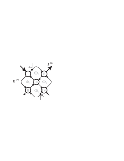
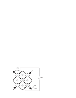
Figure 4: To determine the Hall resistance $R_{\rm H}$ of the RG unit as illustrated here for the $5$SP case the voltage $U$ and the current $J$ are calculated for positive magnetic field $B$ (left) and the opposite direction $-B$ (right). For $-B$ the value of $R_{\rm H}$ can be obtained by measuring $J$ either between the upper (H-flip) or lower (V-flip) two links, respectively.

Assuming that the current enters the RG unit via one incoming link ($I^{\prime}$) only and the other incoming link is inactive ($I^{\prime*}=0$) the resulting power transmission coefficient $t^{\prime 2}=O^{\prime 2}/I^{\prime 2}$ of the RG unit can be associated with $J$. In order to determine $U$ one considers the quantities $a_{u}=O_{1}^{2}/I^{\prime 2}$ and $a_{v}=O_{4}^{*2}/I^{\prime 2}$ as chemical potentials measured by weakly coupled voltage probes at these opposite links of the RG unit [87]. Thus the voltage drop is given by $U=a_{u}-a_{v}$. Because of the four-terminal geometry the obtained $R$ contains beside the Hall resistance $R_{\rm H}$ also a contribution from the longitudinal resistance $R_{\rm L}$. The separation of the unwanted part $R_{\rm L}$ is accomplished by employing the antisymmetry of the Hall voltage $U_{\rm H}$ under the reversal of the direction of the magnetic field $B$

$$U_{\rm H}=\frac{1}{2}\left[U^{(B)}-U^{(-B)}\right].$$ (15)

Considering the $5$SP RG unit again one therefore obtains

$$R_{\rm H}=\frac{1}{2}\frac{\left[a_{u}^{(B)}-a_{v}^{(B)}\right]-\left[a_{u}^{(-B)}-a_{v}^{(-B)}\right]}{t^{\prime 2}}.$$ (16)

The quantities $a_{u}^{(B)}$ and $a_{v}^{(B)}$ are calculated by solving the system of equations (5) analogously to the determination of $t^{\prime}$ in section 2.1. One finds

$$a_{u}^{(B)}=\left|\frac{t_{1}(1-r_{2}r_{3}r_{4}e^{i\Phi_{3}}-t_{3}t_{4}t_{5}e^{i\Phi_{4}})-t_{2}e^{i\Phi_{1}}(t_{3}-t_{4}t_{5}e^{i\Phi_{4}})}{(r_{3}-r_{2}r_{4}e^{i\Phi_{3}})(r_{3}-r_{1}r_{5}e^{i\Phi_{2}})+(t_{3}-t_{4}t_{5}e^{i\Phi_{4}})(t_{3}-t_{1}t_{2}e^{i\Phi_{1}})}\right|^{2}$$ (17)

and

$$a_{v}^{(B)}=\left|\frac{r_{4}(r_{1}r_{3}t_{2}e^{i\Phi_{1}}-r_{5}t_{2}e^{i(\Phi_{1}+\Phi_{2})}+r_{5}t_{1}t_{3}e^{i\Phi_{2}})}{(r_{3}-r_{2}r_{4}e^{i\Phi_{3}})(r_{3}-r_{1}r_{5}e^{i\Phi_{2}})+(t_{3}-t_{4}t_{5}e^{i\Phi_{4}})(t_{3}-t_{1}t_{2}e^{i\Phi_{1}})}\right|^{2}.$$ (18)

Under the reversed field $-B$ the electrons travel along the same equipotentials but in the opposite direction. In the corresponding RG unit the links therefore only change their direction, as shown in Fig. 4. A full rederivation of the RG equation for $-B$ can be omitted if the structure of the RG unit is taken into account. The result with identical directions of the current is obtained by flipping the unit vertically (V-flip) while the other case corresponds to a horizontal flip (H-flip). The comparison to the original RG unit then shows how to map the indices of the SPs and the phases in order to adopt the RG equation to $-B$, which is demonstrated here for the H-flip result where $(r_{1},t_{1})\leftrightarrow(r_{5},t_{5})$, $(r_{2},t_{2})\leftrightarrow(r_{4},t_{4})$, and $\Phi_{1}\leftrightarrow\Phi_{4}$,

$$a_{u}^{(-B)} = \left|\frac{t_{5}(1-r_{2}r_{3}r_{4}e^{i\Phi_{3}}-t_{1}t_{2}t_{3}e^{i\Phi_{1}})-t_{4}e^{i\Phi_{4}}(t_{3}-t_{1}t_{2}e^{i\Phi_{1}})}{(r_{3}-r_{2}r_{4}e^{i\Phi_{3}})(r_{3}-r_{1}r_{5}e^{i\Phi_{2}})+(t_{3}-t_{4}t_{5}e^{i\Phi_{4}})(t_{3}-t_{1}t_{2}e^{i\Phi_{1}})}\right|^{2},$$ (19)

$$a_{v}^{(-B)} = \left|\frac{r_{2}(r_{3}r_{5}t_{4}e^{i\Phi_{4}}-r_{1}t_{4}e^{i(\Phi_{2}+\Phi_{4})}+r_{1}t_{3}t_{5}e^{i\Phi_{2}})}{(r_{3}-r_{2}r_{4}e^{i\Phi_{3}})(r_{3}-r_{1}r_{5}e^{i\Phi_{2}})+(t_{3}-t_{4}t_{5}e^{i\Phi_{4}})(t_{3}-t_{1}t_{2}e^{i\Phi_{1}})}\right|^{2}.$$ (20)

Using Eq. (16) one is now able to determine the distributions of $P(R_{\rm H})$ at the QH transition iteratively in course of the RG iterations.

2.5 Iterating the RG structures

In order to find the FP distribution $P_{\rm c}(t)$, the RG is started from a certain initial distribution of transmission coefficients, $P_{0}(t)$. The distribution is typically discretized in at least $1000$ bins, such that the bin width is typically $0.001$ for the interval $t\in[0,1]$. From $P_{0}(t)$, the $t_{i}$, $i=1,\ldots,5$, are obtained and substituted into the RG transformation (9). The phases $\Phi_{j}$, $j=1,\ldots,4$ are chosen randomly from the interval $\Phi_{j}\in[0,2\pi)$. In this way at least $10^{7}$ super-transmission coefficients $t^{\prime}$ are calculated. In order to decrease statistical fluctuations the obtained histogram $P_{1}(t^{\prime})$ is then smoothed using a Savitzky-Golay filter [85]. At the next step the procedure is repeated using $P_{1}$ as an initial distribution. The convergence of the iteration process is assumed when the mean-square deviation $\int{dt[P_{n}(t)-P_{n-1}(t)]^{2}}$ of the distribution $P_{n}$ and its predecessor $P_{n-1}$ deviate by less than $10^{-4}$.

The actual initial distributions, $P_{0}(t)$, were chosen in such a way that the corresponding conductance distributions, $P_{0}(G)$, were either uniform or parabolic, or identical to the FP distribution found semianalytically [19]. All these distributions are symmetric with respect to $G=0.5$. One can observe that, regardless of the choice of the initial distribution, after $5$–$10$ steps the RG procedure converges to the same FP distribution which remains unchanged for another $4$–$6$ RG steps. Small deviations from the symmetry with respect to $G=0.5$ finally accumulate due to numerical instabilities in the RG procedure, so that typically after $15$–$20$ iterations the distribution becomes unstable and flows toward one of the classical FPs $P(G)=\delta(G)$ or $P(G)=\delta(G-1)$. Therefore the symmetry of the $P_{0}(G)$ with respect to $G=0.5$ is an important requirement in order to converge to the quantum FP at all. Note that the FP distribution can be stabilized by forcing $P_{n}(G)$ to be symmetric with respect to $G=0.5$ in the course of the RG procedure.

Since the dimensionless SP height $z_{i}$ and the transmission coefficient $t_{i}$ at $\varepsilon=0$ are related by Eq. (4), transformation (9) also determines the height of a super-SP by the heights of the five constituting SPs. Correspondingly, the distribution $P(G)$ determines also a distribution $Q(z)$ of the SP heights via $Q(z)=P(G)|dG/dz|=\frac{1}{4}\cosh^{-2}(z/2)P\left[(e^{z}+1)^{-1}\right]$. This represents a convenient parameterization of the conductance distribution, particularly if small and large $t$ values become important. In this case, it is numerically better to perform the RG approach using the $Q(z)$ distribution. We typically discretize the distribution $Q(z)$ in at least $6000$ bins such that the bin width is $0.01$. Since $z\in]-\infty,\infty[$, we have to include lower and upper cut-off SP heights such that $z\in[z_{\rm low},z_{\rm up}]$. From $Q_{0}(z)$, we obtain $z_{i}$, $i=1,\ldots,5$, compute the associated $t_{i}$ and substitute them into the RG transformation (9). At the next step we repeat the procedure using the new $Q_{1}$ as an initial distribution. We check that the values of $z_{\rm low,up}$ do not influence our results.

3 Results of the RG procedure at the QH transition

3.1 Fixed point distributions and the critical exponent

3.1.1 The fixed point distributions $P_{\rm c}(G)$, $Q_{\rm c}(z)$

The distribution $P_{\rm c}(G)$ of the dimensionless conductance $G$ can be obtained from $P(t)$ so that

$$P_{\rm c}(G)\equiv\frac{1}{2t}P_{\rm c}(t)\quad.$$ (21)

Figure 5 illustrates the RG evolution of $P(G)$ and $Q(z)$. In order to reduce statistical fluctuations the FP distribution is averaged over nine results obtained from three different $P_{0}(G)$’s. The FP distribution $P_{\rm c}(G)$ exhibits a flat minimum around $G=0.5$, and sharp peaks close to $G=0$ and $G=1$. It is symmetric with respect to $G\approx 0.5$ with $\langle G\rangle=0.498\pm 0.004$, where the error is the standard error of the mean of the obtained FP distribution. Consequently, the FP distribution $Q_{c}(z)$ is symmetric with respect to $z=0$, which corresponds to the center of the Landau band. The shape of $Q_{c}(z)$ is close to Gaussian. We note that the present results agree with [57, 81, 82] where a similar RG treatment of the CC model was carried out. Our numerical data have a higher resolution, and show significantly less statistical noise because of the faster computation using the analytical solution (9) of the RG[19].

 

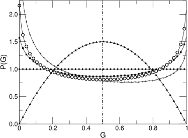
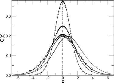
Figure 5: Left: $P(G)$ (thin lines) as function of conductance $G$ at a QH plateau-to-plateau transition. Symbols mark every $20$th data point for different initial distributions ($\blacksquare$,$\blacklozenge$,$\blacktriangle$), the FP distribution ($\bigcirc$) and a distribution for RG step $n=16$ ($+$). The vertical dashed line indicates the average of the FP distribution. Right: Corresponding plots for the distribution $Q(z)$ of SP heights.

3.1.2 The fixed point distributions $P(R_{\rm H})$, $P(R_{\rm L})$

In order to accurately construct the tails of the resistance distributions $P(R_{\rm L})$, $P(R_{\rm H})$, we employ the numerical strategy of section 2.5 and discretize $Q(z)$ with $z_{\rm low}=-20$, $z_{\rm up}=40$ for perturbations towards positive $z$ and vice versa for negative $z$. This corresponds to transmission amplitudes $t(z_{\rm low})\approx 10^{-5}$, $t(z_{\rm up})\approx 1-10^{-9}$ for positive perturbations and vice versa for negative perturbations. Next, we construct via the RG procedure the sequence of distribution $Q_{n}(z)$, $n=1,2,3,\ldots$, calculating at least $10^{8}$ super-transmission coefficients $t^{\prime}$ and associated $z^{\prime}$. We assume that the iteration process has converged when the mean square deviation $\int{dz\left[Q_{n}(z)-Q_{n-1}(z)\right]^{2}}$ of the distribution $Q_{n}$ and its predecessor $Q_{n-1}$ deviate by less than $10^{-4}$. We check that the values of $z_{\rm low,up}$ do not influence our results and that all the previous results at the QH transition as in Refs. [80] are reproduced. The full width at half maximum of the FP distribution $Q_{\rm c}(z)$ is about $5$ [80].

Using Eq. (16) we now obtain besides the FP distribution $Q_{\rm c}(z)$ also the FP distribution $P_{\rm c}(R_{\rm H})$. Like $z$ the value of $R_{\rm H}$ is not bound to a fixed interval. To perform a discretization requires to set lower and upper bounds appropriately. The resulting histogram is limited to $[-100,100]$ containing $40000$ bins. Since $P_{\rm c}(t)$ is already known from section 3.1.1 one can speed up the determination by using $Q_{\rm c}(z)$ as initial $Q_{0}(z)$ and therefore obtain $P_{\rm c}(R_{\rm H})$ already after the first iteration.

In Figure 6 the resulting distributions $P_{\rm c}(R_{\rm L})$ and $P_{\rm c}(R_{\rm H})$ have been plotted. Both distributions are strongly non-Gaussian with long tails. $P_{\rm c}(R_{\rm L})$ can be fitted by a log-normal distribution [37]. We have computed $P_{\rm c}(R_{\rm H})$ using both V- and H-flip structures. Their graphs in Fig. 6 show a significant difference in the shape of $P_{\rm c}(R_{\rm H})$. The H-flip distributions are characterized by a very sharp, nearly symmetric peak at $R_{\rm H}=1$ which coincides with the value of $R_{\rm H}$ at the first Landau level. For V-flip an asymmetric distribution is found again with a strong peak at $R_{\rm H}=1$. Surprisingly, there exists also a kink at $R_{\rm H}=0.5$. Such a peak would normally correspond to a second Landau level, which is however not part of the CC model. The origin of the “wrong” kink must stem from a difference between the calculation of $R_{\rm H}$ according to H-flip and V-flip method, respectively. Both methods differ only in the $(-B)$ part of $R_{\rm H}$. As illustrated in Fig. 4, the H-flip method measures $J$ between the same SPs $I$ and $V$ as for $(+B)$. In contrast, the $J$ for V-flip is obtained between SPs $II$ and $IV$. While one can expect the same result for H-flip and V-flip when considering only the $(-B)$ contribution separately, the final V-flip result for $R_{\rm H}$ according to Eq. (16) thus corresponds to a measurement in a different sample with different random potential. We therefore only use the H-flip results in the following.

 

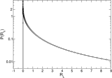
Figure 6: Left: Distribution of the longitudinal resistance $R_{\rm L}$. The $\Box$ symbols indicate the FP distribution, the solid line is a fit to a log-normal distribution for positive $R_{\rm L}$. Only every 5th data point is shown. Right: Distribution of the Hall resistance $R_{\rm H}$ at the FP as obtained from the V-flip (dashed line) and the H-flip method (solid line). Note the kink at $R_{\rm H}=1$ for the V-flip structure.

3.1.3 Critical exponent

The language of the SP heights provides a natural way to extract the critical exponent $\nu$. Suppose that the RG procedure starts with an initial distribution $Q_{0}(z)=Q_{c}(z-z_{0})$ that is shifted from the critical distribution $Q_{c}(z)$ by a small $z_{0}\propto\varepsilon$. The meaning of $z_{0}$ is an additional electron energy measured from the center of the Landau band. The fact that the QH transition is infinitely sharp at $z_{0}=0$ implies that for any $z_{0}\neq 0$, the RG procedure drives the initial distribution $Q(z-z_{0})$ away from the FP. Since $z_{0}\ll 1$, the first RG step would yield $Q_{c}(z-\tau z_{0})$ with some number $\tau$ independent of $z_{0}$. At the $n$th step the center of the distribution will be shifted by $z_{{\rm max},n}=\tau^{n}z_{0}$, while the sample size will be magnified by $2^{n}$. After a certain number of steps, say $n_{L}$, the shift will grow to

$$z_{{\rm max},n_{L}}=\tau^{n_{L}}z_{0}\sim 1$$ (22)

where a typical SP is no longer transmittable. Then the localization length $\xi$ can be identified with the system size $2^{n_{L}}a$ where $a$ is the lattice constant of the original RG unit. Using this relation one can rewrite $\tau^{n_{L}}$ in Eq. (22) as a power of $(\xi/a)$

$$(\xi/a)^{(\ln\tau/\ln 2)}z_{0}\sim 1$$ (23)

from which follows that $\xi$ diverges as

$$\xi\sim az_{0}^{-(\ln 2/\ln\tau)}=az_{0}^{-\nu}$$ (24)

with $\nu=\ln 2/\ln\tau$. When the RG procedure is carried out numerically, one should check that $z_{0}$ is small enough so that $z_{{\rm max},n}\propto z_{0}$ for large enough $n$. Consequently, the working formula for the critical exponent can be presented as

$$\nu=\frac{\ln 2^{n}}{\ln\left(\frac{z_{{\rm max},n}}{z_{0}}\right)}$$ (25)

which should be independent of $n$ for large $n$.

Thus, starting with an initial shift of $Q_{c}(z)$ by a value $z_{0}$ results in the further drift of the maximum position, $z_{{\rm max},n}$, away from $z=0$ after each RG step. As expected, $z_{{\rm max},n}$ depends linearly on $z_{0}$ as shown in Fig. 7 (inset) for different $n$ from $1$ to $8$. The critical exponent is calculated from the slope according to Eq. (25). Its value converges with $n$ to $2.39\pm 0.01$. The error corresponds to a confidence interval of $95\%$ as obtained from the fit to a linear behavior. In Fig. 7, we also show results obtained for the $4$SP structure discussed in section 2.2. Obviously, $\nu_{\rm 4SP}$ tends towards a different value.

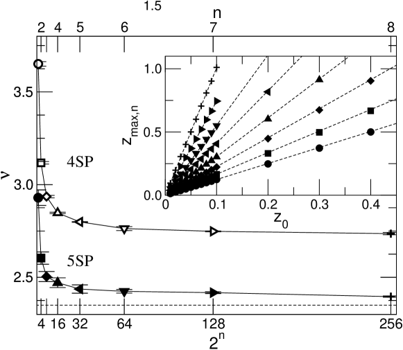
Figure 7: Critical exponent $\nu$ obtained by the QH-RG approach as function of effective linear system size $L=2^{n}$ for RG step $n$. Solid and open symbols correspond to the 5SP and 4SP RG unit, respectively. The error bars correspond to the error of linear fits to the data. The dashed line shows $\nu=2.39$. Inset: $\nu$ (here for 5SP) is determined by the dependence of the maximum $z_{{\rm max},n}$ of $Q_{n}(z)$ on a small initial shift $z_{0}$. Symbols indicate the eight RG steps in accordance with the main plot. Dashed lines indicate the linear fits.

3.1.4 Comparison with other works

By dividing the CC network into units, the RG approach completely disregards at each RG step the interference of the wave-function amplitudes between different units. For this reason it is not clear to what extent this approach captures the main features and reproduces the quantitative predictions at the QH transition. Therefore, a comparison of the RG results with the results of direct simulations of the CC model is crucial. These direct simulations are usually carried out by employing either the quasi-1D version [88, 12, 16] or the 2D version [89, 90, 91, 92] of the transfer-matrix method. For the critical exponent the values $\nu=2.5\pm 0.5$[12] and later $\nu=2.4\pm 0.2$ [16] were obtained. Note that the result of the previous section is in excellent agreement with these values, and is also consistent with the most precise $\nu=2.35\pm 0.03$[14]. This already indicates the remarkable accuracy of the RG approach using the $5$SP structure.

In [93] and [94] $P_{\rm c}(G)$ was studied by methods which are not based on the CC model. Both works reported a broad distribution $P_{\rm c}(G)$. In [90, 91, 92] the critical distribution $P_{\rm c}(G)$ of the conductance was studied. $P_{\rm c}(G)$ was found to be broad, which is in accordance with Fig. 5. One can compare the moments of $P_{\rm c}(G)$ to those calculated in [92, 90]. They agree with the present RG calculations up to the sixth moment. We emphasize that the moments from [92] can hardly be distinguished from the moments of a uniform distribution. This reflects the fact that $P_{\rm c}(G)$ is practically flat except for the peaks close to $G=0$ and $G=1$.

3.2 Energy-level statistics at the QH transition

3.2.1 Choosing an appropriate energy dependence of the phases

The crucial ingredient for obtaining the LSD is the choice of the energy dependence $\Phi_{j}(E)$. If each loop in Fig. 3 is viewed as a closed equipotential as it is the case for the first step of the RG procedure[12], then $\Phi_{j}(E)$ is a true magnetic phase, which changes linearly with energy with a slope governed by the actual potential profile which in turn determines the drift velocity. Thus we make the ansatz

$$\Phi_{j}(E)=\Phi_{0,j}+2\pi\frac{E}{s_{j}},$$ (26)

where a random part $\Phi_{0,j}$ is uniformly distributed within $[0,2\pi)$, and $2\pi/s_{j}$ is a random slope. Here the coefficient $s_{j}$ acts as an initial level spacing connected to the loop $j$ of the RG unit by defining a periodicity of the corresponding phase. Strictly speaking, the dependence (26) applies only for the first RG step. At each step $n>1$, $\Phi_{j}(E)$ is a complicated function of $E$ which carries information about all energy scales at previous steps. However, in the spirit of the RG approach, one can assume that $\Phi_{j}(E)$ can still be linearized within a relevant energy interval. The conventional RG approach suggests that different scales in real space can be decoupled. Linearization of Eq. (26) implies a similar decoupling in energy space. In the case of phases, a “justification” of such a decoupling is that at each RG step, the relevant energy scale, that is the mean level spacing, reduces by a factor of four.

With $\Phi_{j}(E)$ given by Eq. (26), the statistics of energy levels determined by the matrix equation (12) is obtained by averaging over the random initial phases $\Phi_{0,j}$ and values $t_{i}$ chosen randomly according to a distribution $P(t)$. For every realization the levels $E_{k}$ are computed from the solutions $\omega(E_{k})=0$ of Eq. (12) as illustrated in Ref. [83]. The energy interval is scanned in discrete energy steps with $\Delta E=\mbox{min}\{s_{j}\}/250$ which is adapted to each random realization of the $\Phi_{0,j}$ and takes the periodicity in Eq. (26) and its influence on the behavior of $\omega(E)$ into account. In particular, each realization yields three level spacings which are then used to construct a smooth LSD. Thus the situation is comparable with estimating the true RMT ensemble distribution functions from small, say, $2\times 2$ matrices only[84, 95]. The outline of the RG procedure for the LSD is as follows. The slopes $s_{j}$ in Eq. (26) determine the level spacings at the first step. They are randomly distributed with a distribution function $P_{0}(s)$. Subsequent averaging over many realizations yields the LSD, $P_{1}(s)$, at the second step. Then the key element of the RG procedure, as applied to the level statistics, is using $P_{1}(s)$ as a distribution of slopes in Eq. (26). This leads to the next-step LSD and so on.

The approach of this work relies on the “real” eigenenergies of the RG unit. The simpler computation of the spectrum of quasienergies adopted in large-scale simulations within the CC model [15, 17] cannot be applied since the energy dependence of phases $\Phi_{j}$ in the elements of the matrix is neglected and only the random contributions, $\Phi_{0,j}$, are kept. Nevertheless it is instructive to compare the two procedures. In Ref. [83] we have calculated the dependence of the four quasienergies $\omega_{k}$ on the energy $E$ with $t_{i}$ chosen from the critical distribution $P_{\rm c}(t)$. The energy dependence of the phases $\Phi_{j}$ was chosen from LSD of the Gaussian unitary ensemble (GUE) [84, 95] according to Eq. (26). We find that the dependences $\omega(E)$ range from remarkably linear and almost parallel to strongly nonlinear.

3.2.2 The critical LSD at the QH transition

Let us first consider the shape of the LSD at the QH transition. As starting distribution $P_{0}(s)$ of the RG iteration we choose the LSD of GUE because previous simulations [13, 15] indicate that the critical LSD is close to GUE. According to $P_{0}(s)$, each $s_{j}$ is selected randomly and $\Phi_{j}$, $j=1,\ldots,4$ is set as in Eq. (26). For the transmission coefficients of the SP the FP distribution $P_{\rm c}(t)$ is used. As known from section 3.1.1, $P_{n}(t)$ drifts away from the FP within several further iterations due to unavoidable numerical inaccuracies. In order to stabilize the calculation, the FP distribution $P_{\rm c}(t)$ is therefore used in every RG step instead of $P_{n}(t)$. This trick does not alter the results but speeds up the convergence of the RG for $P_{\rm c}(s)$ considerably. By finding solutions $\omega(E_{k})=0$ of Eq. (12) the new LSD $P_{1}(s^{\prime})$ is constructed from the “unfolded” energy level spacings $s^{\prime}_{k}=(E_{k+1}-E_{k})/\Delta$, where $k=1,2,3$, and the mean spacing $\Delta=(E_{4}-E_{1})/3$. Due to the “unfolding”[96] with $\Delta$, the average spacing is set to one for each sample and in each RG-iteration step spacing data of $2\times 10^{6}$ super-SPs are taken into account. The resulting LSD is discretized in bins with largest width $0.01$. In the following iteration step the procedure is repeated using $P_{1}(s)$ as initial distribution. Convergence of the iteration process is assumed when the mean-square deviation of $P_{n}(s)$ deviates by less than $10^{-4}$ from its predecessor $P_{n-1}(s)$. The above approach now enables one to determine the critical LSD $P_{\rm c}(s)$. The RG iteration converges rather quickly after only $2-3$ RG steps. The resulting $P_{\rm c}(s)$ is shown in Fig. 8 together with the LSD for GUE.

 

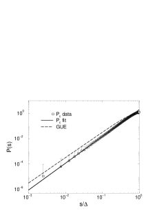
Figure 8: Left: FP distributions $P_{\rm c}(s)$ obtained from the spectrum of $\omega_{l}(E=0)$ and from the RG approach using the real eigenenergies $E_{k}$ in comparison to the LSD $P_{\rm GUE}(s)=32s^{2}\exp{(-\frac{4}{\pi}s^{2})}/\pi^{2}$ for GUE. As in all other graphs $P(s)$ is shown in units of the mean level spacing $\Delta$. Right: $P_{\rm c}(s)$ for small $s$ in agreement with the predicted $s^{2}$ behavior. Due to the log-log plot errors are shown in the upper direction only.

Although $P_{\rm c}(s)$ exhibits the expected features, namely, level repulsion for small $s$ and a long tail at large $s$, the overall shape of $P_{\rm c}(s)$ differs noticeably from GUE. In the previous large-size lattice simulations [13, 15] the obtained critical LSD was much closer to GUE. This fact, however, does not necessarily imply a lower accuracy of the RG approach. Indeed, as it was demonstrated recently, the critical LSD – although being system-size independent — nevertheless depends on the geometry of the samples[97] and on the specific choice of boundary conditions[98, 99]. Sensitivity to the boundary conditions does not affect the asymptotics of the critical distribution, but rather manifests itself in the shape of the “body” of the LSD. One should note that the boundary conditions which have been imposed to calculate the energy levels (dashed lines in Fig. 3) are non-periodic in contrast to usual large-size lattice simulations[15].

As mentioned above there is also the possibility to assess the critical LSD via the distribution of quasienergies. In Fig. 8 the result of this procedure is shown. It appears that the resulting distribution is almost identical to $P_{\rm c}(s)$. This observation is highly non-trivial, since there is no simple relation between the energies and quasienergies [83]. Moreover, choosing another functional form for $\Phi(E)$ instead of the linear $E$-dependence (26), the RG procedure yields an LSD which is markedly different (within the “body”) from $P_{\rm c}(s)$ [83]. Using the quasienergies instead of real energies, as in [15], and linearizing the energy dependence of phases [as in Eq. (26)] is not rigorous. However, the coincidence of the results for the two procedures supports the validity of the approach.

3.2.3 Small-$s$ and large-$s$ behavior

The general shape of the critical LSD is not universal. However, the small-$s$ behavior of $P_{\rm c}(s)$ must be the same as for GUE, namely $P_{\rm c}(s)\propto s^{2}$. This is because delocalization at the QH transition implies level repulsion [100, 101]. Earlier large-scale simulations of the critical LSD [13, 102, 103, 104, 105, 15, 17, 106, 107, 108, 109] satisfy this general requirement. The same holds also for the result of this work, as can be seen in Fig. 8. The given error bars of the numerical data are standard deviations computed from a statistical average of $100$ FP distributions each obtained for different random sets of $t_{i}$’s and $\Phi_{j}$’s within the RG unit. In general, within the RG approach, the $s^{2}$-asymptotics of $P(s)$ is most natural. This is because the levels are found from diagonalization of the $4\times 4$ unitary matrix (13) with absolute values of elements widely distributed between $0$ and $1$.

The right form of the large-$s$ tail of $P(s)$ is Poissonian with $P_{\rm c}(s)\propto\exp(-bs)$ [101, 103, 13, 110]. It appears that the accuracy of the present RG approach is insufficient to discern this non-trivial feature of the critical LSD, since we have a good accuracy only for $s/\Delta\lesssim 2.5$ [83].

3.2.4 Finite-size scaling at the QH transition

In order to extract $\nu$ from the LSD the one-parameter-scaling hypothesis [111] is employed. The approach describes the rescaling of a quantity $\alpha(N;\{z_{i}\})$ — depending on (external) system parameters $\{z_{i}\}$ and the system size $N$ — onto a single curve by using a scaling function $f$

$$\alpha\left(N;\{z_{i}\}\right)=f\left(\frac{N}{\xi_{\infty}(\{z_{i}\})}\right).$$ (27)

We now use the scaling assumption to extrapolate $f$ to $N\rightarrow\infty$ from the finite-size results of the computations. The knowledge about $f$ and $\xi_{\infty}$ then allows to derive the value of $\nu$ similarly to (24). In order to define a suitable control parameter $z_{0}$ in the transition region, again the natural parameterization (4) of the transmission coefficients is used. Because the QH transition occurs exactly at $z_{0}=0$ any initial distribution $Q(z-z_{0})$ with $z_{0}\neq 0$ will evolve during the RG procedure toward an insulator, either with complete transmission of the network nodes (for $z_{0}>0$) or with complete reflection of the nodes (for $z_{0}<0$).

In principle, one is free to choose for the finite-size scaling (FSS) analysis any characteristic quantity $\alpha(N;z_{0})$ constructed from the LSD which has a systematic dependence on system size $N$ for $z_{0}\neq 0$ while being constant at the transition $z_{0}=0$. Out of the large number of possible choices[13, 112, 101, 113, 114, 110] a restriction is made to quantities that are defined mainly by the small-$s$ behavior which is accurately described by the RG approach. The quantities are obtained by integration of the LSD and have already been successfully used in [115, 112, 113], namely

$$\alpha_{\rm P}=\int^{s_{0}}_{0}P(s)ds,\quad\alpha_{\rm I}=\frac{1}{s_{0}}\int^{s_{0}}_{0}I(s)ds,\quad\alpha_{\rm S}=\int^{\infty}_{0}s^{2}P(s)ds$$ (28)

with $I(s)=\int^{s}_{0}P(s^{\prime})ds^{\prime}$. The integration limit for the first 2 quantities is chosen as $s_{0}=1.4$ which approximates the common crossing point[112] of all LSD curves as can be seen in Fig. 9.

Figure 9: RG of the LSD used for the computation of $\nu$. The dotted lines corresponds to the first $9$ RG iterations with an initial distribution $P_{0}$ shifted to the metallic regime ($z_{0}=0.1$) while the full thin lines represent results for a shift toward localization ($z_{0}=-0.1$). Within the RG procedure the LSD moves away from the FP as indicated by the arrows. At $s/\Delta\approx 1.4$ the curves cross at the same point which is used when deriving a scaling quantity from the LSD.

Thus $P(s_{0})$ is independent of the distance $|z-z_{\rm c}|$ to the critical point and the system size $N$. Note that $N$ is directly related to the RG step $n$ by $N=2^{n}$. The double integration in $\alpha_{\rm I}$ is numerically advantageous since fluctuations in $P(s)$ are smoothed. One can now apply the finite-size-scaling approach from Eq. (27) for $\alpha_{\rm P,I,S}(N,z_{0})$. Since $\alpha_{\rm P,I,S}(N,z_{0})$ is analytical for finite $N$, one can expand the scaling function $f$ at the critical point. The first-order approximation yields

$$\alpha(N,z_{0})\sim\alpha(N,z_{\rm c})+a|z_{0}-z_{\rm c}|N^{1/\nu}$$ (29)

where $a$ is a coefficient. Better results are obtained using a higher-order expansion proposed by Slevin and Ohtsuki[116], but contributions from an irrelevant scaling variable can be neglected since the transition point $z_{0}=0$ is known [83].

In order to obtain the functional form of $f$ the fitting parameters, including $\nu$, are evaluated by a nonlinear least-square ($\chi^{2}$) optimization. In Fig. 10 the resulting fits for, e.g., $\alpha_{\rm S}$ at the transition are shown. The fits are chosen such that the total number of parameters is kept small and the fit agrees well with the numerical data. The corresponding scaling curve is displayed in the right panel of Fig. 10. In the plots the two branches for complete reflection ($z_{0}<0$) and complete transmission ($z_{0}>0$) can be distinguished clearly. In order to estimate the error of the fitting procedure the over $100$ results for $\nu$ obtained by different orders of the expansion, system sizes $N$, and $z$ ranges around the transition are compared [83, 117]. The value of $\nu=2.37\pm 0.02$ is calculated as average over many individual fits for $\alpha_{\rm P,I}$. It is in excellent agreement with $2.39\pm 0.01$ calculated in section 3.1.3. The value obtained from the parameter-free scaling quantity $\alpha_{\rm S}=\int_{0}^{\infty}s^{2}P(s)ds$[113] is $\nu=2.33\pm 0.05$, but scaling is less reliable due to the insufficient statistics in the large-$s$ tail.

 

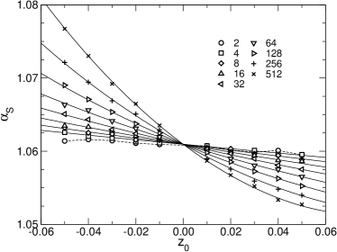
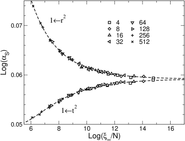
Figure 10: Behavior of $\alpha_{\rm S}$ at the QH transition. Left: Data for RG iterations $n=1,\ldots,9$ corresponding to effective system sizes $N=2^{n}=2,\ldots,512$. Full lines indicate the functional dependence according to FSS using the $\chi^{2}$ minimization with ${\cal O}_{\nu}=2$ and ${\cal O}_{z}=3$. Because of large deviations data for $N=2$ were excluded from the fitting. Right: Resulting FSS curves. Different symbols correspond to different effective system sizes $N=2^{n}$.

Finally the influence of the initial conditions on the result of the LSD and the one-parameter scaling has been studied in Ref. [83]. The corresponding LSD agrees with GUE less convincingly than the LSD computed using the true $P_{\rm c}(G)$. Estimates of the critical exponent yield also less accurate values $\nu_{\rm I}=2.43\pm 0.02$ and $\nu_{\rm P}=2.46\pm 0.03$ which are nevertheless still reasonably close to $\nu=2.37\pm 0.02$. Thus our choice of the initial distribution $P_{\rm c}(G)$ is indeed valid.

4 Extensions of the RG approach

4.1 The QH-to-insulator transition

4.1.1 Evolution of the resistance distributions $P(R_{\rm L})$ and $P(R_{\rm H})$

In order to model the transition into the insulating regime, we shift the initial distribution $Q_{0}(z)\rightarrow Q_{0}(z-z_{0})$ by a small $z_{0}$. For $z_{0}<0$ and $z_{0}>0$, the RG flow will then drive the distributions into the insulating, $G\rightarrow 0$, and plateau, $G\rightarrow 1$, regimes, respectively. In Fig. 11, we show the resulting distributions after many RG steps. For $P(R_{\rm L})$, we see in Fig. 11 that the flow towards $G\rightarrow 1$ results in a decrease of large $R_{\rm L}$ events, whereas conversely, the regime $G\rightarrow 0$ leads to an increase in large $R_{\rm L}$ values and a decrease of the maximum value in $P(R_{\rm L})$. For $P(R_{\rm H})$, Fig. 11 shows that the plateau regime $G\rightarrow 1$ gives a highly singular peak at the dimensionless quantized Hall value $1$, corresponding to a perfect Hall plateau. On the other hand, the insulating regime $G\rightarrow 0$ shows an increase of weight in the tails of $P(R_{\rm H})$ and the eventual obliteration of any central peak.

 

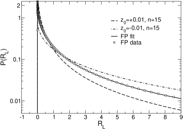
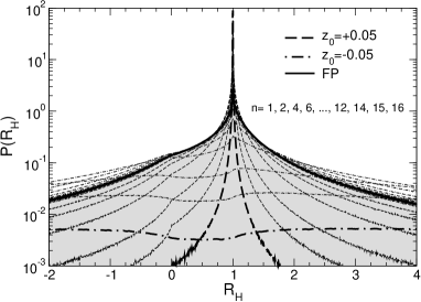
Figure 11: Left: Distribution of the longitudinal resistance $R_{\rm L}$. The $\Box$ symbols indicate the FP distribution, the solid line is a fit to a log-normal distribution and the dot-dashed and dashed lines show the distribution after $n=15$ RG iterations into the conductance regimes $G(z_{0}<0)\rightarrow 0$ and $G(z_{0}>0)\rightarrow 1$. Only every 5th data point is shown for $P(R_{\rm L})$. Right: Distribution of the Hall resistance $R_{\rm H}$. The FP distribution has been shaded to zero. For the $G(z_{0}<0)\rightarrow 0$ and $G(z_{0}>0)\rightarrow 1$ regimes, we have indicated the distributions after $n=16$ RG iterations by bold dashed and dot-dashed lines.

Very large absolute values of $R_{\rm L}$ and $R_{\rm H}$ in the tails are obviously the consequence of a very small denominator $t^{\prime 2}$ in Eqs. (14) and (16) meaning that the current is almost totally reflected by the RG unit. This scenario is possible since $P_{n}(t^{2})$ also exhibits strong fluctuations and spreads over the whole range between $0$ and $1$.

4.1.2 Evolution of the average resistances

In order to extract an averaged $R_{\rm L}$ and $R_{\rm H}$ from these non-standard distributions, we should now select an appropriate mean $\langle\cdot\rangle$ that characterizes and captures the essential physics and allows comparison with the experimental data. The precise operational definition is also important as it corresponds to different possible experimental setups. Therefore, we consider several means: (i) arithmetic $\langle R\rangle_{\rm ari}=\sum_{i}R_{i}/N$, (ii) geometric/typical $\langle R\rangle_{\rm typ}=\exp\sum_{i}\ln R_{i}/N$, (iii) median (central value) $\langle R\rangle_{\rm med}$, where $N$ denotes the number of samples ($\gtrsim 10^{8}$) in each case. The median and the typical mean (and their variances [38]) are less sensitive to extreme values than other means (such as, e.g. root-mean-square and harmonic mean) and this makes them a better measure for highly skewed and long-tailed distributions such as $P(R_{\rm L})$ and $P(R_{\rm H})$ in the insulating regime. In the plateau regimes, the distributions are less skewed, particularly for $R_{\rm H}$ and the difference in the means becomes less important.

We are left with determining in which operational order to apply the averaging procedure. For $R_{\rm L}$, as measured via Ohm’s law (14) as a ratio, it is obvious that the appropriate average should be ${R}_{\rm L}=\frac{1}{\langle G\rangle}-1$ (and not $\langle\frac{1}{G}\rangle-1$). For $R_{\rm H}$, the situation is less straightforward due to the definition of $U_{\rm H}$ in (16). A simple average is $\langle U_{\rm H}\rangle$, i.e. using the appropriate $P(R_{\rm H})$. Similar to the experimental procedure, we can also estimate $U_{\rm H}$ via $\langle a_{u}-a_{v}\rangle$ for each $B$ field direction separately. In Ref. [38], it has been suggested that a more appropriate average $\langle U_{\rm H}\rangle^{*}$ can be constructed from $\langle a_{u}\rangle-\langle a_{v}\rangle$. This later procedure corresponds to measuring the voltage drop between positions $a_{u}$ and $a_{v}$ in Fig. 3 by separately measuring the individual voltages with respect to ground and then recombining them. For $R_{\rm H}$, this yields

$$\langle R_{\rm H}\rangle_{\rm typ}^{*}=\frac{1}{2}\frac{\left(\langle a_{u}^{(B)}\rangle_{\rm typ}-\langle a_{v}^{(B)}\rangle_{\rm typ}\right)-\left(\langle a_{u}^{(-B)}\rangle_{\rm typ}-\langle a_{v}^{(-B)}\rangle_{\rm typ}\right)}{\langle t^{\prime 2}\rangle_{\rm typ}}.$$ (30)

 

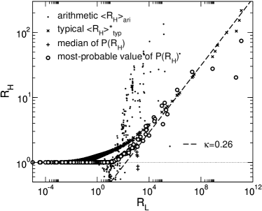
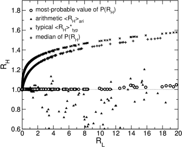
Figure 12: Left: Dependence of averaged $R_{\rm H}$ on averaged $R_{\rm L}$ for various means obtained from $10^{8}$ samples. The dashed line describes the divergence $R_{\rm H}\propto R_{\rm L}^{\kappa}$ of the typical mean $\langle R_{\rm H}\rangle^{*}_{\rm typ}$, the median $\langle R_{\rm H}\rangle_{\rm med}$ and the most probable value of $P(R_{\rm H})$. The variance of the arithmetic mean diverges as $R_{\rm L}\rightarrow\infty$ and $\langle R_{\rm H}\rangle_{\rm ari}$ is no longer a useful characteristic of $P(R_{\rm H})$. The horizontal dotted line indicates $R_{\rm H}=1$. Right: Plot of the same data as in Fig. 12 but on a linear scale and for experimentally accessible resistance values. Here the almost quantized behavior for the most probable value of $P(R_{\rm H})$ becomes even more pronounced. The horizontal dotted line indicates $R_{\rm H}=1$.

In Fig. 12 we show the resulting dependence $R_{\rm H}(R_{\rm L})$ when these averaging definitions are being used. In the plateau regime $R_{\rm L}<1$, the nearly constant behavior of all $R_{\rm H}$ averages is as expected. For $R_{\rm L}\rightarrow\infty$, we get a divergent $R_{\rm H}$ when using the median and typical means as suggested by Refs. [37, 38] to compute both $R_{\rm L}$ and $R_{\rm H}$. This divergence can be captured by a power-law $R_{\rm H}\propto R_{\rm L}^{\kappa}$ with $\kappa\approx 0.26$. The arithmetic mean for large $R_{\rm L}\gg 1$ quickly becomes instable and no useful information can be inferred.

Reducing the information to the experimentally more relevant resistance regime of a few times $h/e^{2}$, we replot the $R_{\rm L}$ and $R_{\rm H}$ data in Fig. 12 (right panel) on a linear scale. In addition to the three means above, we also show the behavior of the most-probable value $\hat{R}_{\rm H}$ at which $P(R_{\rm H})$ has a maximum. This estimate $\hat{R}_{\rm H}(R_{\rm L})$ appears relevant in the experimental setup where $10^{8}$ different samples cannot be easily measured and the full distribution functions cannot be constructed in similar detail. Most importantly, for the range of $R_{\rm L}$ values shown in Fig. 12, the value of $\hat{R}_{\rm H}$ deviates only slightly from its quantized value $1$ at the transition and $R_{\rm L}+R_{\rm H}\approx R_{\rm 2t}$ [36]. Therefore, the experimental estimate of $R_{\rm H}$ appears to support the notion of the quantized Hall insulator. Indeed, the deviations from $1$ are less than $10\%$ until $R_{\rm L}\sim 25$. However, going back to the left panel of Fig. 12, we see that in the strongly insulating regime $R_{\rm L}\rightarrow\infty$ also $\hat{R}_{\rm H}$ diverges with a power-law that is well-described by $\langle R\rangle^{*}_{\rm typ}$. We emphasize that fluctuations in $\hat{R}_{\rm H}$ for large ${R}_{\rm L}\gg 10^{5}$ are due to numerical inaccuracies in $P(R_{\rm H})$ and decrease upon further increasing the number of samples.

The results for $R_{\rm L}$ and $R_{\rm H}$ in the localized regime can be very well described by an exponential scaling function with finite-size correction [37] $R_{\rm L,H}(2^{n},z)\propto 2^{\gamma n}\exp[{2^{n}}{\xi^{-1}_{\rm L,H}(z)}]$. Plotting $\xi_{\rm L,H}$ as a function of small perturbation $z_{0}$, we find $\xi_{\rm L,H}(z_{0})\propto z_{0}^{-\nu_{\rm L,H}}$ with $\nu_{\rm L,H}\approx 2.35$ as shown in Fig. 13. Thus we recover the universal divergence of the localization length $\xi$ even when using the RG in the insulating regime [14].

 

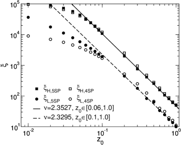
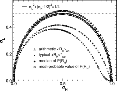
Figure 13: Left: Dependence of the localization lengths $\xi_{L}$ and $\xi_{H}$ on the initial shift $z_{0}$ using the ansatz (8) of [37]. We obtain a reasonable estimate of the critical exponent $\nu$. Right: The semi circle law for different means as in Fig. 12. The most probable values ($\circ$) show perfect semi-circle (solid line) behavior. The thin dotted line denotes $\sigma_{\rm L}={1}/{2}$.

An equally reliable estimate of the irrelevant exponent $\gamma$ appears not possible for our data. As usual, the 4-terminal resistances can be converted into the respective conductances via $\sigma_{\rm L,H}={R_{\rm L,H}}/\left({R_{\rm L}^{2}+R_{\rm H}^{2}}\right)$. For these conductances, one expects the semi-circle law $\sigma_{\rm L}^{2}+\left(\sigma_{\rm H}-{1}/{2}\right)^{2}=\left({1}/{2}\right)^{2}$ to hold [52]. In Fig. 13, we show that the most-probable values capture the overall shape and symmetry properties best [25, 36], the other averages show pronounced deviations. We also note that the relation $R_{\rm L}(z_{0})=1/R_{\rm L}(-z_{0})$ is obeyed by all means [118]. This is a consequence of the reflection symmetry of $P(G)$ [80].

4.2 Macroscopic inhomogeneities in the RG approach

4.2.1 Implementing power-law correlations in the RG approach

A natural way to incorporate a quenched disorder into the CC model is to ascribe a certain random shift, $z_{Q}$, to each SP height, and to assume that the shifts at different SP positions, ${\bf r}$ and ${\bf r}^{\prime}$, are correlated as

$$\langle z_{Q}({\bf r})z_{Q}({\bf r}^{\prime})\rangle\propto|{\bf r}-{\bf r}^{\prime}|^{-\alpha},$$ (31)

with $\alpha>0$. After this, the conventional transfer-matrix methods of [89, 88] could be employed for numerically precise determination of $\langle G\rangle$, the distribution $P_{\rm c}(G)$, its moments, and most importantly, the critical exponent, $\nu$. However, the transfer-matrix approach for a 2D sample is usually limited to fairly small cross sections (e.g., up to $128$ in [91]) due to the numerical complexity of the calculation. Therefore, the spatial decay of the power-law correlation by, say, more than an order in magnitude is hard to investigate for small $\alpha$.

On the other hand, the RG approach is perfectly suited to study the role of the quenched disorder. First, after each step of the RG procedure, the effective system size doubles. At the same time, the magnitude of the smooth potential, corresponding to the spatial scale $r$, falls off with $r$ as $r^{-\alpha/2}$. As a result, the modification of the RG procedure due to the presence of the quenched disorder reduces to a scaling of the disorder magnitude by a constant factor $2^{-\alpha/2}$ at each RG step. Second, the RG approach operates with the conductance distribution $P_{n}(G)$ which carries information about all the realizations of the quenched disorder within a sample of size $2^{n}$. This is in contrast to the transfer-matrix approach[89, 88], within which a small increase of the system size requires the averaging over the quenched disorder realizations to be conducted again.

The above consideration suggests the following algorithm. For the homogeneous case all SPs constituting the new super-SP are assumed to be identical, which means that the distribution of heights, $Q_{n}(z)$, for all of them is the same. For the correlated case these SPs are no longer identical, but rather their heights are randomly shifted by the long-ranged potential. In order to incorporate this potential into the RG scheme, $Q_{n}(z_{i})$ should be replaced by $Q_{n}(z_{i}-\Delta^{(n)}_{i})$ for each SP, $i$, where $\Delta^{(n)}_{i}$ is the random shift. Then the power-law correlation of the quenched disorder enters into the RG procedure through the distribution of $\Delta^{(n)}_{i}$. That is, for each $n$ the distribution is Gaussian with the width $\beta(2^{n})^{-\alpha/2}$. For large enough $n$ the critical behavior should not depend on the magnitude of the correlation strength $\beta$, but on the power, $\alpha$, only.

4.2.2 A new critical behavior

We find that for all values of $\alpha>0$ in correlator (31) the FP distribution is identical to the uncorrelated case within the accuracy of the calculation. In particular, $\langle G\rangle=0.498$ is unchanged. However, the convergence to the FP is numerically less stable than for uncorrelated disorder due to the correlation-induced broadening of $Q_{n}(z)$ during each iteration step. In order to compute the critical exponent $\nu(\alpha)$ the RG procedure is started from $Q_{0}(z-z_{0})$, as in the uncorrelated case, but in addition the random shifts are incorporated. As already explained these shifts are a result of the quenched disorder in generating the distribution of $z$ at each RG step. The outcome is shown in Fig. 14. It illustrates that for increasing long-ranged character of the correlation (decreasing $\alpha$) the convergence to a limiting value of $\nu$ slows down drastically. Even after eight RG steps (i.e., a magnification of the system size by a factor of $256$), the value of $\nu$ with long-ranged correlations still differs appreciably from $\nu=2.39$ obtained for the uncorrelated case. The RG procedure becomes unstable after eight iterations, i.e., $z_{\rm{max},9}$ can no longer be obtained reliably from $Q_{9}(z)$. Unfortunately, for small $\alpha$ the convergence is too slow to yield the limiting value of $\nu$ after eight steps only. For this reason, the above method is, strictly speaking, unable to unambiguously answer the question whether sufficiently long-ranged correlations result in an $\alpha$-dependent critical exponent $\nu(\alpha)$, or whether the value of $\nu$ eventually approaches the uncorrelated value of $2.39$. Nevertheless, the results in Fig. 14 indicate that the effective critical exponent exhibits a sensitivity to the long-ranged correlations even after a large magnification by $256\times 256$. Since this factor coincides with the change in scale from the microscopic magnetic length to the realistic samples with finite sizes of several $\mu{\rm m}$, macroscopic inhomogeneities are able to affect the results of scaling studies.

 

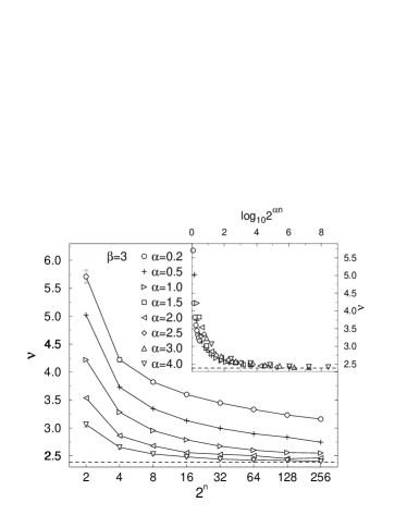
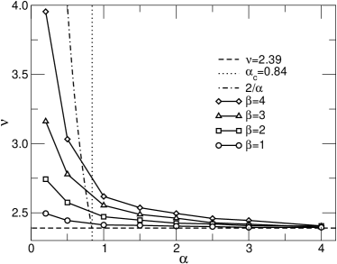
Figure 14: Left: Critical exponent $\nu$ obtained by the QH-RG approach as a function of RG scale $2^{n}$ for $\beta=3$ and different correlation exponents $\alpha$. The dashed line indicates $\nu=2.39$, which is the value obtained for uncorrelated disorder. For clarity, the errors are shown only for $\alpha=0.2$ and $4$. Inset: $\nu$ vs $2^{\alpha n/2}$ shows deviations from scaling. Right: Dependence of the critical exponent $\nu$ on correlation exponent $\alpha$ for different $\beta=1,2,3$, and $4$ as obtained after eight QH-RG iterations. The dotted line indicates $\alpha_{\rm c}=0.84$. The dot-dashed line $\nu=2/\alpha$ for $\alpha<\alpha_{\rm c}$ follows from the extended Harris criterion [119] for classical percolation.

Note further that as shown in the inset of Fig. 14 one can observe scaling of $\nu$ values when plotted as function of a renormalized system size $2^{\alpha n/2}$ only for large correlation strength $\beta$. In this case the disorder broadening during the first RG steps becomes comparable to the FP distribution. Therefore in the QH-RG the correlated disorder dominates over the initial FP distribution. One should emphasize that $\nu(\alpha)$ obtained after eight RG steps always exceeds the uncorrelated value.

Figure 14 shows the values of $\nu$ obtained after the eighth RG step as a function of the correlation exponent $\alpha$ for different dimensionless strengths $\beta$ of the quenched disorder. It is seen that in the domain of $\alpha$, where the values of $\nu$ differ noticeably from $\nu=2.39$, their dependence on $\beta$ is strong. According to the extended Harris criterion [119, 120], $\nu(\alpha)$ is expected to exhibit a cusp at the $\beta$-independent value $\alpha_{c}=2/2.39\approx 0.84$. From the results in Fig. 14, two basic observations can be made. For a small enough magnitude of the long-range disorder, one observes a smooth enhancement of $\nu(\alpha)$ with decreasing $\alpha$ without a cusp. Although such a behavior might be caused by the relatively small number of RG steps, the data can be relevant for realistic samples which have a finite size and a finite phase-breaking length governed by temperature. At the largest $\beta=4$, there is still no clear cusp but the $\alpha$-dependence for $\alpha<\alpha_{\rm c}$ is closer to the $\nu=2/\alpha$ predicted by the extended Harris criterion. Unfortunately, the numerics becomes progressively unstable, forbidding to go to even larger $\beta$.

4.2.3 Intrinsic short-range disorder in quantum percolation

Here one should note that there is a crucial distinction between the classical case and the quantum regime of the electron motion considered in the present RG approach. In this study, the correlation of the heights of the SPs has been incorporated into the RG scheme. At the same time it was assumed that the Aharonov-Bohm phases acquired by an electron upon traversing the neighboring loops are uncorrelated. This assumption implies that, in addition to the long-ranged potential, a certain short-ranged disorder causing a spread in the perimeters of neighboring loops of the order of the magnetic length is present in the sample. The consequence of this short-range disorder is the sensitivity of the results to the value of $\beta$ which parametrizes the magnitude of the correlated potential. The presence of this short-range disorder affecting exclusively the Aharonov-Bohm phases significantly complicates the observation of the cusp in the $\nu(\alpha)$ dependence at $\alpha\approx 0.84$, as is expected from the extended Harris criterion. A more detailed investigation of this effect has been given in Ref. [80]. We emphasize that an unambiguous demonstration of the validity of the extended Harris criterion has recently been given by the Liouville approach to the random Landau matrix model [121].

5 Conclusions

Real-space RG approaches to problems of quantum statistical physics have been applied with much success in many context. The RG necessarily uses only a local approximation to the full connectivity of the network. Thus it is important to choose the RG structures such that the overall symmetries of the network are retained. In the present work, we have shown various examples where such a strategy is permissible in the context of the integer QH effect. Particularly for the determination of critical distributions $P_{\rm c}(G)$, $P_{\rm c}(R_{\rm L})$, $P_{\rm c}(R_{\rm H})$ and the critical exponent $\nu=2.39\pm 0.01$, this allowed us to study of the critical properties of the QH transition with surprisingly high accuracy. It seems possible to further enhance the accuracy of the RG by increasing the size of the RG unit [82]. However, in order to fully benefit from the increased size, it is essential that an analytic solution as in Eq. (9) is obtained. Otherwise, numerical round-off and stability effects will lead to an overall decreased accuracy. We emphasize also that in the case of larger RG units the size-rescaling factor needs to be calculated with care.

The robustness of the 5SP RG when computing universal properties is moreover demonstrated by an FSS analysis of the LSD around the QH transition. The exponent $\nu=2.37\pm 0.02$ of the localization length obtained by a nonlinear $\chi^{2}$ minimization is in excellent agreement with the value reported in the literature. It is surprisingly good when keeping in mind that it was derived just from the four loops of the RG unit which therefore seem to capture the essential physics of the QH transition. The success of the RG approach to the LSD can be attributed to the description of the transmission amplitudes $t$ of the SPs by a full distribution function $P(t)$ while for network models usually a fixed value $t(E)$ is assigned to all SPs for simplicity. Also, the phases are associated with full loops in the network and not with single SP-SP links. Due to these reasons the RG iteration is always governed by the quantum critical point of the QH transition. Even when starting the iteration with a distribution $P_{0}(G)$ totally different from $P_{\rm c}(G)$, but still symmetric with respect to $G=0.5$, one approaches the same results after a few iterations.

Having established that the RG approach works at the QH transition, we then set out to extend the method to distributions away from criticality. We have shown in a quantum coherent calculation that the insulating Hall behavior of $R_{\rm H}(R_{\rm L}\rightarrow\infty)$ is dominated by the power-law divergence $R_{\rm H}\propto R_{\rm L}^{\kappa}$. However, in the experimentally attained range $R_{\rm L}\leq 10$ [25, 26, 36], the deviation from a quantized $R_{\rm H}=1$ is very small and the onset of the divergence for $R_{\rm L}\gg 10$ is yet to be explored.

It was argued for a long time that the enhanced value of the critical exponent $\nu$ extracted from the narrowing of the transition region with temperature [122, 34] has its origin in the long-ranged disorder present in GaAs-based samples. To our knowledge, the present RG approach was the first attempt to quantify this argument. As a result the random potential with a power-law correlator leads to values of $\nu$ exceeding $\nu\approx 2.35$.

The result indicates that macroscopic inhomogeneities must lead to smaller values of $\kappa\propto 1/\nu$. Experimentally, the value of $\kappa$ smaller than $0.42$ was reported in a number of early (see, e.g., [123] and references therein) as well as recent [124] works. This fact was accounted for by different reasons (such as temperature dependence of the phase breaking time, incomplete spin resolution, valley degeneracy in Si-based MOSFETs, and inhomogeneity of the carrier concentration in GaAs-based structures with a wide spacer). Briefly, the spread of the $\kappa$ values was attributed to the fact that the temperatures were not low enough to assess the truly critical regime. The possibility of having $\kappa<0.4$ due to the correlation-induced dependence of the effective $\nu$ on the phase-breaking length or, ultimately, on the sample size, as in Fig. 14, was not considered.

It should be pointed out that the limited number of RG steps permitted by the numerics nevertheless allows one to trace the evolution of the wave functions from microscopic scales (of the order of the magnetic length) to macroscopic scales (of the order of several $\mu{\rm m}$) which are comparable to the sizes of the samples used in the experimental studies of scaling (see e.g., [125, 123]) and much larger than the samples[126, 127] used for the studies of mesoscopic fluctuations. Another qualitative conclusion of this study is that the spatial scale at which the exponent $\nu$ assumes its “infinite-sample” value is much larger in the presence of the quenched disorder than in the uncorrelated case. In fact this scale can be of the order of microns. This conclusion can also have serious experimental implications. That is, even if the sample size is much larger than this characteristic scale, this scale can still exceed the phase-breaking length, which would mask the true critical behavior at the QH transition.

Let us briefly comment on the possible future application of the method. An obvious possibility is the application to extended variants of the standard CC model, e.g. a network with at least two channels per link in order to describe the mixing of Landau levels [53]. There remain several interesting questions such as the behavior of the critical properties at the QH transition when changing from strong to weak magnetic field. This case could be modelled by bi-directional links in the network, which would allow one to trace the transition from the universality class GUE to GOE. And last, but certainly not least, we have described the integer QH effect within a non-interacting electron picture, but experimental results clearly indicate the influence of interactions [128, 31]. Because a full treatment of many-body interactions is rather difficult one might consider in an approximate view only a few interacting particles. In this approach the two-interacting particle problem is reduced to a single-particle problem by increasing the effective spatial dimension and including long-range correlations in the disorder potential[129]. Concerning the CC model one has to construct an effective four-dimensional network. From this new CC network a suitable RG unit should be extracted. This tasks are by no means trivial but first steps have already been undertaken [130].

References

- [1] K. v. Klitzing, G. Dorda, and M. Pepper, Phys. Rev. Lett. 45, 494 (1980).
- [2] D. C. Tsui, H. L. Störmer, and A. C. Gossard, Phys. Rev. Lett. 48, 1559 (1982).
- [3] T. Chakraborty and P. Pietilänen, The Quantum Hall Effects (Springer, Berlin, 1995).
- [4] D. Yoshioka, The Quantum Hall Effect, Springer Series in Solid-State Sciences 133 (Springer, Berlin, 2002).
- [5] H. Aoki and T. Ando, Solid State Commun. 38, 1079 (1981).
- [6] M. Janssen, O. Viehweger, U. Fastenrath, and J. Hajdu, Introduction to the Theory of the Integer Quantum Hall effect (VCH, Weinheim, 1994).
- [7] R. B. Laughlin, Phys. Rev. B 23, 5632 (1981).
- [8] R. E. Prange, Phys. Rev. B 23, 4802 (1981).
- [9] A. M. M. Pruisken, Nucl. Phys. B 235, 277 (1984).
- [10] D. J. Thouless, M. Kohmoto, M. P. Nightingale, and M. d. Nijs, Phys. Rev. Lett. 49, 405 (1982).
- [11] B. Huckestein, Rev. Mod. Phys. 67, 357 (1995).
- [12] J. T. Chalker and P. D. Coddington, J. Phys.: Condens. Matter 21, 2665 (1988).
- [13] M. Batsch and L. Schweitzer, in High Magnetic Fields in Physics of Semiconductors II: Proceedings of the International Conference, Würzburg 1996, edited by G. Landwehr and W. Ossau (World Scientific Publishers Co., Singapore, 1997), pp. 47–50, ArXiv: cond-mat/9608148.
- [14] B. Huckestein, Europhys. Lett. 20, 451 (1992).
- [15] R. Klesse and M. Metzler, Phys. Rev. Lett. 79, 721 (1997).
- [16] D.-H. Lee, Z. Wang, and S. Kivelson, Phys. Rev. Lett. 70, 4130 (1993).
- [17] M. Metzler, J. Phys. Soc. Japan 67, 4006 (1998).
- [18] D. P. Arovas, M. Janssen, and B. Shapiro, Phys. Rev. B 56, 4751 (1997), ArXiv: cond-mat/9702146.
- [19] A. G. Galstyan and M. E. Raikh, Phys. Rev. B 56, 1422 (1997).
- [20] J. J. Binney, N. J. Dowrick, A. J. Fisher, and M. E. J. Newman, The Theory of Critical Phenomena: An Introduction to the Renormalization Group (Oxford University Press, Oxford, UK, 1992).
- [21] K. G. Wilson, Rev. Mod. Phys. 55, 583 (1983).
- [22] J. L. Cardy, Scaling and Renormalization in Statistical Physics (Cambridge University Press, Cambridge, 1996).
- [23] M. Salmhofer, Renormalization: an Introduction (Springer, Berlin, 1999).
- [24] V. J. Goldman, J. K. Wang, B. Su, and M. Shayegan, Phys. Rev. Lett. 70, 647 (1993).
- [25] M. Hilke et al., Nature 395, 675 (1998).
- [26] D. d. Lang et al., Physica E 12, 666 (2002).
- [27] D. Shahar et al., Solid State Commun. 102, 817 (1997).
- [28] D. Shahar et al., Science 274, 589 (1996).
- [29] R. Hughes et al., J. Phys.: Condens. Matter 6, 4763 (1994).
- [30] S. Q. Murphy et al., Physica E 6, 293 (2000).
- [31] W. Pan et al., Phys. Rev. B 55, 15431 (1997).
- [32] D. Shahar et al., Phys. Rev. Lett. 74, 4511 (1995).
- [33] D. Shahar et al., Phys. Rev. Lett. 79, 479 (1997).
- [34] R. T. F. v. Schaijk et al., Phys. Rev. Lett. 84, 1567 (2000).
- [35] E. Shimshoni, Mod. Phys. Lett. B 18, 923 (2004).
- [36] E. Peled et al., Phys. Rev. Lett. 90, 246802 (2003).
- [37] L. P. Pryadko and A. Auerbach, Phys. Rev. Lett. 82, 1253 (1999).
- [38] U. Zülicke and E. Shimshoni, Phys. Rev. B 63, 241301 (2001), ArXiv: cond-mat/0101443.
- [39] F. Evers, A. D. Mirlin, D. G. Polyakov, and P. Wölfle, Phys. Rev. B 60, 8951 (1999).
- [40] N. R. Cooper, B. I. Halperin, C.-K. Hu, and I. M. Ruzin, Phys. Rev. B 55, 4551 (1997).
- [41] I. M. Ruzin, N. R. Cooper, and B. I. Halperin, Phys. Rev. B 53, 1558 (1996).
- [42] E. Shimshoni, Phys. Rev. B 60, 10691 (1999).
- [43] E. Shimshoni, A. Auerbach, and A. Kapitulnik, Phys. Rev. Lett. 80, 3352 (1998).
- [44] S. H. Simon and B. I. Halperin, Phys. Rev. Lett. 73, 3278 (1994).
- [45] M. Janssen, M. Metzler, and M. R. Zirnbauer, Phys. Rev. B 59, 15836 (1999).
- [46] V. Kagalovsky, B. Horovitz, and Y. Avishai, Phys. Rev. B 52, R17044 (1995).
- [47] V. Kagalovsky, B. Horovitz, and Y. Avishai, Phys. Rev. B 55, 7761 (1997).
- [48] R. Klesse and M. Metzler, Europhys. Lett. 32, 229 (1995).
- [49] R. Klesse and M. R. Zirnbauer, Phys. Rev. Lett. 86, 2094 (2001), ArXiv: cond-mat/0010005.
- [50] D. K. K. Lee and J. T. Chalker, Phys. Rev. Lett. 72, 1510 (1994).
- [51] D. K. K. Lee, J. T. Chalker, and D. Y. K. Ko, Phys. Rev. B 50, 5272 (1994).
- [52] I. Ruzin and S. Feng, Phys. Rev. Lett. 74, 154 (1995).
- [53] Z. Wang, D.-H. Lee, and X.-G. Wen, Phys. Rev. Lett. 72, 2454 (1994).
- [54] S. V. Iordanskii, Solid State Commun. 43, 1 (1982).
- [55] D. Stauffer and A. Aharony, Perkolationstheorie (VCH, Weinheim, 1995).
- [56] S. Koch, R. J. Haug, K. v. Klitzing, and K. Ploog, Phys. Rev. B 43, 6828 (1991).
- [57] M. Janssen, R. Merkt, J. Meyer, and A. Weymer, Physica 256–258, 65 (1998).
- [58] B. Huckestein and B. Kramer, Phys. Rev. Lett. 64, 1437 (1990).
- [59] Y. Huo and R. N. Bhatt, Phys. Rev. Lett. 68, 1375 (1992).
- [60] M. Büttiker, Y. Imry, R. Landauer, and S. Pinhas, Phys. Rev. B 31, 6207 (1985).
- [61] B. Shapiro, Phys. Rev. Lett. 48, 823 (1982).
- [62] J. T. Chalker et al., Phys. Rev. B 65, 012506 (2002), ArXiv: cond-mat/0009463.
- [63] P. Freche, M. Janssen, and R. Merkt, in Proceedings of the Ninth International Conference on Recent Progress in Many Body Theories, edited by D. Neilson (World Scientific, Singapore, 1998), ArXiv: cond-mat/9710297.
- [64] P. Freche, M. Janssen, and R. Merkt, Phys. Rev. Lett. 82, 149 (1999).
- [65] M. Janssen, Phys. Rep. 295, 1 (1998).
- [66] V. Kagalovsky, B. Horovitz, Y. Avishai, and J. T. Chalker, Phys. Rev. Lett. 82, 3516 (1999).
- [67] R. Merkt, M. Janssen, and B. Huckestein, Phys. Rev. B 58, 4394 (1998).
- [68] I. A. Gruzberg, N. Read, and S. Sachdev, Phys. Rev. B 55, 10593 (1997).
- [69] C.-M. Ho and J. T. Chalker, Phys. Rev. B 54, 8708 (1996), ArXiv: cond-mat/9605073.
- [70] Y. B. Kim, Phys. Rev. B 53, 16420 (1996).
- [71] J. Kondev and J. B. Marston, Nucl. Phys. B 497, 639 (1997), ArXiv: cond-mat/9612223.
- [72] D.-H. Lee, Phys. Rev. B 50, 10788 (1994).
- [73] A. W. W. Ludwig, M. P. A. Fisher, R. Shankar, and G. Grinstein, Phys. Rev. B 50, 7526 (1994).
- [74] J. B. Marston and S. Tsai, Phys. Rev. Lett. 82, 4906 (1999).
- [75] M. R. Zirnbauer, Ann. Phys. (Leipzig) 3, 513 (1994).
- [76] M. R. Zirnbauer, J. Math. Phys. 38, 2007 (1997), ArXiv: cond-mat/9701024.
- [77] J. Bernasconi, Phys. Rev. B 18, 2185 (1978).
- [78] P. J. Reynolds, W. Klein, and H. E. Stanley, J. Phys. C 10, L167 (1977).
- [79] D. Stauffer and A. Aharony, Introduction to Percolation Theory (Taylor and Francis, London, 1992).
- [80] P. Cain, R. A. Römer, M. Schreiber, and M. E. Raikh, Phys. Rev. B 64, 235326 (2001), ArXiv: cond-mat/0104045.
- [81] M. Janssen, R. Merkt, and A. Weymer, Ann. Phys. (Leipzig) 7, 353 (1998).
- [82] A. Weymer and M. Janssen, Ann. Phys. (Leipzig) 7, 159 (1998), ArXiv: cond-mat/9805063.
- [83] P. Cain, R. A. Römer, and M. E. Raikh, Phys. Rev. B 67, 075307 (2003), ArXiv: cond-mat/0209356.
- [84] M. L. Mehta, Random Matrices and the Statistical Theory of Energy Levels (Academic Press, New York, 1991).
- [85] W. H. Press, B. P. Flannery, S. A. Teukolsky, and W. T. Vetterling, Numerical Recipes in FORTRAN, 2nd ed. (Cambridge University Press, Cambridge, 1992).
- [86] H. A. Fertig, Phys. Rev. B 38, 996 (1988).
- [87] C. W. J. Beenakker and H. van Hoiuten, in Solid State Physics: Advances in Research and Applications, edited by H. Ehrenreich and D. Turnbull (Academic, San Diego, 1991), Vol. 44, p. 207.
- [88] A. MacKinnon and B. Kramer, Phys. Rev. Lett. 47, 1546 (1981).
- [89] D. S. Fisher and P. A. Lee, Phys. Rev. B 23, 6851 (1981).
- [90] S. Cho and M. P. A. Fisher, Phys. Rev. B 55, 1637 (1997).
- [91] B. Jovanovic and Z. Wang, Phys. Rev. Lett. 81, 2767 (1998).
- [92] Z. Wang, B. Jovanovic, and D.-H. Lee, Phys. Rev. Lett. 77, 4426 (1996).
- [93] X. Wang, Q. Li, and C. M. Soukoulis, Phys. Rev. B 58, 3576 (1998).
- [94] Y. Avishai, Y. Band, and D. Brown, Phys. Rev. B 60, 8992 (1999).
- [95] E. P. Wigner, Proc. Camb. Phil. Soc. 47, 790 (1951).
- [96] F. Haake, Quantum Signatures of Chaos, 2nd ed. (Springer, Berlin, 1992).
- [97] H. Potempa and L. Schweitzer, J. Phys.: Condens. Matter 10, L431 (1998), ArXiv: cond-mat/9804312.
- [98] D. Braun, G. Montambaux, and M. Pascaud, Phys. Rev. Lett. 81, 1062 (1998), ArXiv: cond-mat/9712256.
- [99] L. Schweitzer and H. Potempa, Physica A 266, 486 (1998), ArXiv: cond-mat/9809248.
- [100] Y. V. Fyodorov and A. D. Mirlin, Phys. Rev. B 55, 16001 (1997).
- [101] B. I. Shklovskii et al., Phys. Rev. B 47, 11487 (1993).
- [102] M. Batsch, L. Schweitzer, and B. Kramer, Physica B 249, 792 (1998), ArXiv: cond-mat/9710011.
- [103] M. Batsch, L. Schweitzer, I. K. Zharekeshev, and B. Kramer, Phys. Rev. Lett. 77, 1552 (1996), ArXiv: cond-mat/9607070.
- [104] M. Feingold, Y. Avishai, and R. Berkovits, Phys. Rev. B 52, 8400 (1995), ArXiv: cond-mat/9503058.
- [105] T. Kawarabayashi, T. Ohtsuki, K. Slevin, and Y. Ono, Phys. Rev. Lett. 77, 3593 (1996), ArXiv: cond-mat/9609226.
- [106] M. Metzler, J. Phys. Soc. Japan 68, 144 (1999).
- [107] M. Metzler and I. Varga, J. Phys. Soc. Japan 67, 1856 (1998).
- [108] T. Ohtsuki and Y. Ono, J. Phys. Soc. Japan 64, 4088 (1995), ArXiv: cond-mat/9509146.
- [109] Y. Ono, T. Ohtsuki, and B. Kramer, J. Phys. Soc. Japan 65, 1734 (1996), ArXiv: cond-mat/9603099.
- [110] I. K. Zharekeshev and B. Kramer, Phys. Rev. Lett. 79, 717 (1997), ArXiv: cond-mat/9706255.
- [111] E. Abrahams, P. W. Anderson, D. C. Licciardello, and T. V. Ramakrishnan, Phys. Rev. Lett. 42, 673 (1979).
- [112] E. Hofstetter and M. Schreiber, Phys. Rev. B 49, 14726 (1994), ArXiv: cond-mat/9402093.
- [113] I. K. Zharekeshev and B. Kramer, Jpn. J. Appl. Phys. 34, 4361 (1995), ArXiv: cond-mat/9506114.
- [114] I. K. Zharekeshev and B. Kramer, Phys. Rev. B 51, 17239 (1995).
- [115] E. Hofstetter and M. Schreiber, Phys. Rev. B 48, 16979 (1993).
- [116] K. Slevin and T. Ohtsuki, Phys. Rev. Lett. 82, 382 (1999), ArXiv: cond-mat/9812065.
- [117] P. Cain, Ph.D. thesis, Technische Universität Chemnitz, 2004.
- [118] D. Shahar et al., Solid State Commun. 107, 19 (1998), ArXiv: cond-mat/9706045.
- [119] A. Weinrib and B. I. Halperin, Phys. Rev. B 27, 413 (1983).
- [120] A. Weinrib, Phys. Rev. B 29, 387 (1984).
- [121] N. Sandler, H. R. Maei, and J. Kondev, Phys. Rev. B 68, 205315 (2003), ArXiv: cond-mat/0304616.
- [122] H. P. Wei, S. Y. Lin, D. C. Tsui, and A. M. M. Pruisken, Phys. Rev. B 45, 3926 (1992).
- [123] S. Koch, R. J. Haug, K. v. Klitzing, and K. Ploog, Phys. Rev. B 46, 1596 (1992).
- [124] G. Landwehr, private communication.
- [125] S. Koch, R. J. Haug, K. v. Klitzing, and K. Ploog, Phys. Rev. Lett. 67, 883 (1991).
- [126] D. H. Cobden, C. H. W. Barnes, and C. J. B. Ford, Phys. Rev. Lett. 82, 4695 (1999).
- [127] D. H. Cobden and E. Kogan, Phys. Rev. B 54, R17316 (1996).
- [128] L. W. Engel, D. Shahar, C. Kurdak, and D. C. Tsui, Phys. Rev. Lett. 71, 2638 (1993).
- [129] D. L. Shepelyansky, Phys. Rev. Lett. 73, 2607 (1994).
- [130] V. Apalkov and M. E. Raikh, Phys. Rev. B 68, 195312 (2003), arXiv: cond-mat/0303170.