Dynamics of Shuttle Devices

Andrea Donarini

Ph.D. Thesis

Technical University of Denmark

phd

Foreword

This thesis is submitted in candidacy for the Ph.D. degree within the Physics Program at the Technical University of Denmark. The thesis describes part of the work that I have carried out under supervision of Antti-Pekka Jauho from the Department of Micro and Nanotechnology.

I’m grateful to my supervisor for the very stimulating atmosphere that he has been able to create and maintain within his group and also for his gentle but firm guidance. I want to thank all the members of the Theoretical Nanotechnology Group at the MIC Department and in particular Dr. Tomáš Novotný and Christian Flindt for the close and intense collaboration that has generated a large part of the results presented in this thesis.

I would like to thank Prof. Timo Eirola for having introduced me to the subject of the iterative numerical methods and for his precious help in the solution of some of the numerical problems I encounter in my research. I want also to thank Dr. Tobias Brandes and Neill Lambert for the nice physics discussions I could have with them during the period I spent collaborating with them in Manchester. I want to thank Christian Flindt also for the enthusiasm and the very positive attitude that he has been always able to spread within the “Shuttle Group”. He has also been an indefatigable reader of the proofs and deserves many thanks for that. Finally I also want to thank my family for their far but constant support and all the Italian friends in Copenhagen for being very patient and encouraging me during the writing period.

Lyngby, September 3, 2004

Andrea Donarini

phd

Preface

Much interest has been drawn in recent years to the concept and realization of Nanoelectromechanical systems (NEMS). NEMS are nanoscale devices that combine mechanical and electrical dynamics in a strong interplay. The shuttle devices are a particular kind of Nanoelectromechanical systems. The characteristic component that gives the name to these devices is an oscillating quantum dot of nanometer size that transfers electrons one-by-one between a source and a drain lead. The device represents the nano-scale analog of an electromechanical bell in which a metallic ball placed between the plates of a capacitor starts to oscillate when a high voltage is applied to the plates.

This thesis contains the description and analysis of the dynamics of two realizations of quantum shuttle devices. We describe the dynamics using the Generalized Master Equation approach: a well-suited method to treat this kind of open quantum systems. We also classify the operating modes in three different regimes: the tunneling, the shuttling and the coexistence regime. The characterization of these regimes is given in terms of three investigation tools: Wigner distribution functions, current and current-noise. The essential dynamics of these regimes is captured by three simplified models whose derivation from the full description is possible due to the time scale separation of the particular regime. We also obtain from these simplified models a more intuitive picture of the variety of different dynamics exhibited by the shuttle devices.

Lyngby, October 10, 2004

Andrea Donarini

phd

Chapter 1 Introduction

In this chapter we give a short introduction to the world of nanoelectromechanical systems. We then focus our attention on a particular kind of device called electron shuttle. We sketch the basic operating regime and give an overview of the different theoretical models that have been proposed to describe the dynamics of such devices. We report on the two main realizations of shuttle devices and close the chapter with an outline of the contents of this thesis.

1.1 NEMS

Much interest has been drawn in recent years on the concepts and realization of Nanoelectromechanical systems (NEMS). NEMS are nanoscale devices that combine mechanical and electrical dynamics in a strong interplay. This property makes them interesting both from a technological and fundamental point of view. They are extremely sensitive mass and position detectors. Due to their very high mechanical frequency one can even think of using them as the basis for new form of mechanical computers. From the point of view of fundamental research they represent extremely good tools to probe directly the basic quantum mechanical laws. They could represent the first man-made structures on which the mechanical zero point fluctuation can be detected. They also rise the question on the limiting dimension for persistence of mechanical coherence. In general one of the fascinating aspects of these objects is their mesoscopic character: they share with the macroscopic world the large number of atoms of which they are made (typically of millions of atoms) but on the other hand their behaviour is (or should be) already significantly determined by quantum mechanics.

1.2 A new transport regime

The shuttle devices are a particular kind of NEMS. The characteristic component that gives the name to these devices is an oscillating object of nanometer size that transfers electrons one-by-one between a source and a drain lead. The device represents the nano-scale analog of an electromechanical bell in which a metallic ball placed between the plates of a capacitor starts to oscillate when a high voltage is applied to the plates. The oscillations are sustained by the external bias that pumps energy into the mechanical system: when the ball is in contact with the negatively biased plate it gets charged and the electrostatic field drives it towards the other capacitor plate where the ball releases the electrons and returns back due to the oscillator restoring forces and the cycle starts again.

In the first proposal [1] of a shuttle device the movable carrier is a metallic grain confined into a harmonic potential by elastically deformable organic molecular links attached to the leads. The transfer of charge is governed by tunneling events, the tunneling amplitude being modulated by the position of the oscillating grain. The exponential dependence of the tunneling amplitude of the grain position leads to an alternating opening and closing of the left and right tunneling channels that resembles the charging and discharging dynamics of the macroscopic analog.

Different models for shuttle devices have been proposed in the literature since this first seminal work by Gorelik et al. [1]. The mechanical degree of freedom has been treated classically (using harmonic [2, 3, 4, 5] or more realistic potentials [6]) and quantum mechanically [7, 8, 9]. Armour and MacKinnon proposed a model with the oscillating grain flanked by two static quantum dots [7, 10, 11, 12]. More generally the shuttling mechanism has been applied to Cooper pair transport [13, 14] and pumping of superconducting phase [15] or magnetic polarization [16].

The essential feature of the nano-scale realization is the quantity transferred per cycle (a charge up to $10^{10}$ electrons for a macroscopic bell) that is scaled down to 1 quantum unit (electron, spin, Cooper pair in the different realizations). We can already guess the basic properties of the shuttle transport:

1. Charge-position correlation: the shuttling dot loads the charge on one side and transfers it on the other side, it releases it and returns back to the starting point;

2. Matching between electronic and mechanical characteristic times (non-adiabaticity);

3. Quantized current determined by the mechanical frequency;

4. Low current fluctuations: the stochasticity of the tunneling event is suppressed due to an interplay between mechanical and electrical properties. The tunneling event is only probable at some particular short time periods fixed by the mechanical dynamics (i.e. when the oscillating dot is close to a specific lead).

1.3 Experimental implementations

An experimental realization of the shuttle device has been produced by Erbe et al. [17]. The structure consists of a cantilever with a quantum island at the top placed between source and drain leads. Two lateral gates can set the cantilever into motion via a capacitive coupling. An ac voltage applied at these gates makes the cantilever vibrating and brings the tip alternatively closer to the source or drain lead and thus allows the shuttling of electrons.

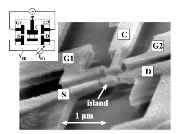
Figure 1.1: Electron micrograph of the nano-mechanical resonator. The cantilever (C) can be set into motion by applying an ac-voltage between the two gates G1 and G2, and by applying a bias across the metallic tip of the cantilever (the island) electrons are shuttled from the source (S) to the drain (D). The picture is taken from [17].

The device (shown in Fig. 1.1) is built out of silicon-on-insulator (SOI) materials (using Au for the metallic parts) using etch mask techniques and optical and electron beam lithography. The cantilever is $~{}1\mu m$ long and the corresponding resonant frequency is of the order of $100{\,\rm MHz}$. The source electrode and the cantilever are at an average distance of approximately $0.1\,\mu m$. Shuttling experiments have been performed by Erbe et al. at different temperatures. For experiments at $4.2\,{\rm K}$ and $12\,{\rm K}$ they measured a pronounced peak in the current through the cantilever for a driving frequency of approximately $120\,{\rm MHz}$ corresponding to the natural frequency of the first mode of the oscillator. The peak in the current corresponds to a rate of shuttle success of about one electron per 9 mechanical cycles. The Erbe experiment is very close to the original proposal by Gorelik. The only difference is in the external driving of the mechanical oscillations. In the original proposal the bias was time independent and the driving induced by the electrostatic force on the charged oscillating island. The initially stochastic tunneling events would eventually cause the shuttling instability and drive the system into a self-sustained mechanical oscillation combined with periodic charging and discharging events.

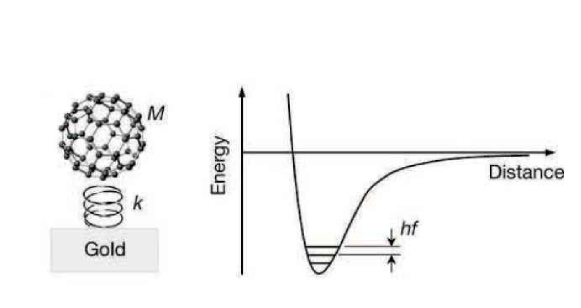
Figure 1.2: The C₆₀ experiment by Park et al. The C₆₀ molecule (of mass M) can be considered as being attached to a spring with spring constant $k$ and corresponding quantized excitation energy $hf$ of the order of 5 meV. The figure is taken from [18].

Another experiment often mentioned in the context of quantum shuttles is the C₆₀-experiment by Park et al. [18] In this experiment a C₆₀ molecule is deposited in the gap between two gold electrodes. The gap, produced with break junction technique, has a width of 1 nm. The molecule (of diameter 0.7 nm) is bound to the electrodes due to van der Waals interaction. Around the equilibrium position the potential can be approximated by a harmonic potential and the molecule can be considered as attached by springs. We show a schematic representation of this idea in Fig. 1.2. In the experiment Park et al. sweep the voltage across the junction and register sudden increases in the current. The steps are separated by 5 meV. Since the lowest internal excitation energy of the C₆₀ molecule is $35$ meV one concludes that the slower center of mass motion could be involved in the process. This hypothesis is confirmed by the fact that the separation between the steps is independent of the charge on the C₆₀ molecule and the theoretical estimate for the energy corresponding to the center of mass oscillation in the van der Waals potential is exactly 5 meV. The IV-curve measured in these experiments can be interpreted in terms of shuttling [19], but also alternative explanations have been promoted [20, 21, 22]. Whether we are in presence of coherent or incoherent shuttling transport and to what extent the shuttling mechanism is involved in this set-up cannot be completely clarified by current measurement. The current-current correlation (also called current noise) was proposed by Fedorets et al. [19] for a better understanding of the underlying dynamics of the current jumps. For this reason the calculation of noise in shuttle devices has been performed by many different groups. We proposed a completely quantum formulation [23] that is also explained in detail in this thesis.

1.4 This thesis

This thesis contains the description and analysis of the dynamics of two realizations of quantum shuttle devices. The models we consider describe both the mechanical and electrical degrees of freedom quantum mechanically. For the single dot quantum shuttle we extended an existing classical model proposed by Gorelik et al. [1]. For the triple dot case we adopted the model invented by Armour and MacKinnon [7]. In the following we outline the contents of the thesis:

In Chapter 2 we introduce the two models called Single Dot Quantum Shuttle and Triple Dot Quantum Shuttle, the first being the quantum extension also for the mechanical degree of freedom of the model originally proposed by Gorelik et al. [1] while the second is the model invented by Armour and MacKinnon [7]. Also in this model the oscillator is treated quantum mechanically and the central moving dot is flanked by two static dots.

We dedicate Chapter 3 to the derivation of the Generalized Master Equation (GME) that describes the shuttle device dynamics. Due to the different coupling strengths we treat the mechanical and electrical baths with two different approaches. The Gurvitz approach for the electrical and the standard Born-Markov approximation for the mechanical bath. The derivation à la Gurvitz represents a large part of this chapter. In order to facilitate the understanding of this non-standard method and appreciate our extension to the shuttle device we have given a long introduction in which we analyze in great detail simpler models with increasing physical complexity. This shows on one hand the essence of the derivation in simpler cases and also underlines the potentiality of this approach. An important aspect of this method is also to be a natural prelude to full counting statistics since it naturally produces a GME that counts the number of electron which tunneled through the device at a certain time. We close the chapter with the description of the numerical iterative method that we adopted for the calculation of the stationary solution of the GME.

In Chapter 4 we introduce the concept of Wigner distribution function and derive the corresponding Klein-Kramers equation for the SDQS starting from the GME that we obtained in the previous chapter. The Wigner function description is motivated by the effort to keep the complete quantum treatment we achieved with the GME without losing as much as possible the intuitive classical picture and with the possibility to handle the quantum-classical correspondence.

Chapter 5 is dedicated to the definition and application of the three investigation tools we have chosen to analyze the properties of shuttle devices: the charge resolved phase-space distribution, the current and the current-noise. The phase space analysis reveals the shuttling transition and the charge position correlation typical of this operating regime. It also gives a very clean way to appreciate “geometrically” the quantum to classical transition of the shuttling behaviour for different device realizations. The second investigation tool that we consider is the current. From the current calculation we obtain also in the quantum treatment the quantized value of one electron per cycle found in the semiclassical treatments of similar devices. We then present current-noise calculations based on the MacDonald formula. The derivation is strongly dependent on the derivation à la Gurvitz of the $n$-resolved GME. The low noise quasi-deterministic behaviour of the shuttling transport is clear from the extremely low Fano factors found for this regime. In general we are able with all the three investigation tools to identify three operating regimes of shuttle devices: the tunneling, shuttling and coexistence regimes.

Chapter 6 is dedicated to a qualitative description of the these regimes and also to the identification of the relation between different times and length scales that define the three regimes in terms of the model parameters.

In Chapter 7 we consider separately the tunneling, shuttling and coexistence regime. The specific separation of time scales allows us to identify the relevant variables and describe each regime by a specific simplified model. Models for the tunneling, shuttling and coexistence regime are analyzed in this chapter. We also give a comparison with the full description in terms of Wigner distributions, current and current-noise to prove that the models, at least in the limits set by the chosen investigation tools, capture the relevant dynamics.

A summary of the arguments treated in this thesis opens Chapter 8. We conclude with a list of some of the open questions that could encourage a continuation of the present work.

Chapter 2 The models

We describe in this chapter two models of quantum shuttles: the Single-Dot Quantum Shuttle and the Triple-Dot Quantum Shuttle. Due to the nanometer size of these devices we decide to treat quantum mechanically not only the electrical but also the mechanical dynamics. This approach was suggested by the work of Armour and MacKinnon [7] for the triple dot device and implemented for the first time by us in the single dot device.

2.1 Single-Dot Quantum Shuttle

The Single-Dot Quantum Shuttle (SDQS) consists of a movable quantum dot (QD) suspended between source and drain leads. One can imagine the dot attached to the tip of a cantilever or connected to the leads by some soft legands or embedded into an elastic matrix. In the model the center of mass of the nanoparticle is confined to a potential that, at least for small diplacements from its equilibrium position, can be considered harmonic. We give a schematic visualization of the device in figure 2.1.

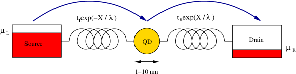
Figure 2.1: Schematic representation of the Single-dot Shuttle: electrons tunnel from the left lead at chemical potential ($\mu_{L}$) to the quantum dot and eventually to the right lead at lower chemical potential $\mu_{R}$. The position dependent tunneling amplitudes are indicated. $X$ is the displacement from the equilibrium position. The springs represent the harmonic potential in which the central dot can move.

Due to its small diameter, the QD has a very small capacitance and thus a charging energy that exceeds (in the most recent realizations almost at room temperature [24]) the thermal energy $k_{B}T$. For this reason we assume that only one excess electron can occupy the device (Coulomb blockade) and we describe the electronic state of the central dot as a two-level system (empty/charged). Electrons can tunnel between leads and dot with tunneling amplitudes which are exponentially dependent on the position of the central island. This is due to the exponentially decreasing/increasing overlapping of the electronic wave functions.

The Hamiltonian of the model reads:

$$H=H_{\rm sys}+H_{\rm leads}+H_{\rm bath}+H_{\rm tun}+H_{\rm int}$$ (2.1)

where

$$\begin{split}&H_{\rm sys}=\frac{\hat{p}^{2}}{2m}+\frac{1}{2}m\omega^{2}\hat{x}^{2}+(\varepsilon_{1}-e\mathcal{E}\hat{x})c_{1}^{{\dagger}}c_{1}^{\phantom{\dagger}}\\ &H_{\rm leads}=\sum_{k}(\varepsilon_{l_{k}}c^{\dagger}_{l_{k}}c^{\phantom{\dagger}}_{l_{k}}+\varepsilon_{r_{k}}c^{\dagger}_{r_{k}}c^{\phantom{\dagger}}_{r_{k}})\\ &H_{\rm tun}=\sum_{k}[T_{l}(\hat{x})c^{\dagger}_{l_{k}}c_{1}^{\phantom{\dagger}}+T_{r}(\hat{x})c^{\dagger}_{r_{k}}c_{1}^{\phantom{\dagger}}]+h.c.\\ &H_{\rm bath}+H_{\rm int}={\rm generic\;heat\;bath}\end{split}$$ (2.2)

Using the language of quantum optics we call the movable grain alone the system. This is then coupled to two electric baths (the leads) and a generic heat bath. The system is described by a single electronic level of energy $\varepsilon_{1}$ and a harmonic oscillator of mass $m$ and frequency $\omega$. When the dot is charged the electrostatic force ($e\mathcal{E}$) acts on the grain and gives the electrical influence on the mechanical dynamics. The electric field $\mathcal{E}$ is generated by the voltage drop between left and right lead. In our model, though, it is kept as an external parameter, also in view of the fact that we will always assume the potential drop to be much larger than any other energy scale of the system (with the only exception of the charging energy of the dot). The operator form $\hat{x},\hat{p}$ for the mechanical variables is due to the quantum treatment of the harmonic oscillator. In terms of creation and annihilation operators for oscillator excitations we would write:

$$\begin{split}&\hat{x}=\sqrt{\frac{\hbar}{2m\omega}}(d^{\dagger}+d)\\ &\hat{p}=i\sqrt{\frac{\hbar m\omega}{2}}(d^{\dagger}-d)\\ &\frac{\hat{p}^{2}}{2m}+\frac{1}{2}m\omega^{2}\hat{x}^{2}=\hbar\omega\left(d^{\dagger}d+\frac{1}{2}\right)\end{split}$$ (2.3)

The leads are Fermi seas kept at two different chemical potentials ($\mu_{L}$ and $\mu_{R}$) by the external applied voltage ($\Delta V=(\mu_{L}-\mu_{R})/e$ ). The oscillator is immersed into a dissipative environment that we model as a collection of bosons and is coupled to that by a weak bilinear interaction:

$$\begin{split}H_{\rm bath}&=\sum_{\mathbf{q}}\hbar\omega_{\mathbf{q}}{d_{\mathbf{q}}}^{\dagger}d_{\mathbf{q}}\\ H_{\rm int}&=\sum_{\mathbf{q}}\hbar g({d_{\mathbf{q}}}+{d_{\mathbf{q}}}^{\dagger})(d+d^{\dagger})\end{split}$$ (2.4)

where the bosons have been labelled by their wave number $\mathbf{q}$. The damping rate is given by:

$$\gamma(\omega)=2\pi g^{2}D(\omega)$$ (2.5)

where $D(\omega)$ is the density of states for the bosonic bath at the frequency of the system oscillator. A bath that generates a frequency independent $\gamma$ is called Ohmic.

The coupling to the electric baths is introduced by the tunneling Hamiltonian $H_{\rm tun}$. The tunneling amplitudes $T_{l}(\hat{x})$ and $T_{r}(\hat{x})$ depend exponentially on the position operator $\hat{x}$ and represent the mechanical feedback on the electrical dynamics:

$$T_{l,r}(\hat{x})=t_{l,r}\exp(\mp\hat{x}/\lambda)$$ (2.6)

where $\lambda$ is the tunneling length. The tunneling rates from and to the leads ($\bar{\Gamma}_{L,R}$) can be expressed in terms of the amplitudes:

$$\bar{\Gamma}_{L,R}=\langle\Gamma_{L,R}(\hat{x})\rangle=\left\langle\frac{2\pi}{\hbar}D_{L,R}\exp\left(\mp\frac{2\hat{x}}{\lambda}\right)|t_{l,r}|^{2}\right\rangle$$ (2.7)

where $D_{L,R}$ are the densities of states of the left and right lead respectively and the average is taken with respect to the quantum state of the oscillator.

The model presents three relevant time scales: the period of the oscillator $2\pi/\omega$, the inverse of the damping rate $1/\gamma$ and the average injection/ejection time $1/\bar{\Gamma}_{L,R}$. It is possible also to identify three important length scales: the zero point uncertainty $\Delta x_{z}=\sqrt{\frac{\hbar}{2m\omega}}$, the tunneling length $\lambda$ and the displaced oscillator equilibrium position $d=\frac{e\mathcal{E}}{m\omega^{2}}$. Different relations between time and length scales distinguish different operating regimes of the SDQS.

2.2 Triple-Dot Quantum Shuttle

The Triple-Dot Quantum Shuttle (TDQS) was proposed by Armour and MacKinnon [7]. The system consists of an array of three QD’s: a movable dot, that we assume confined to a harmonic potential, flanked by two static ones. Relying on low temperature and on the low capacitance of the system with respect to the leads, we again assume strong Coulomb blockade: only one electron at a time can occupy the three-dot device. The Hamiltonian for the model reads:

$$H=H_{\rm sys}+H_{\rm leads}+H_{\rm bath}+H_{\rm tun}+H_{\rm int}$$ (2.8)

Only the system and tunneling part of the Hamiltonian differ from the one dot case:

$$\begin{split}H_{\rm sys}=&\epsilon_{0}|0\rangle\!\langle 0|+\frac{\Delta V}{2}|L\rangle\!\langle L|-\frac{\Delta V}{2x_{0}}\hat{x}|C\rangle\!\langle C|-\frac{\Delta V}{2}|R\rangle\!\langle R|+\hbar\omega\left(d^{{\dagger}}d+\frac{1}{2}\right)\\ &+t_{R}(\hat{x})(|C\rangle\!\langle R|+|R\rangle\!\langle C|)+t_{L}(\hat{x})(|C\rangle\!\langle L|+|L\rangle\!\langle C|)\\ H_{\rm tun}=&\sum_{k}T_{l}(c^{\dagger}_{l_{k}}|0\rangle\!\langle L|+c^{\phantom{\dagger}}_{l_{k}}|L\rangle\!\langle 0|)+T_{r}(c^{\dagger}_{r_{k}}|0\rangle\!\langle R|+c^{\phantom{\dagger}}_{r_{k}}|R\rangle\!\langle 0|)\end{split}$$ (2.9)

where $H_{\rm osc}$ is the harmonic-oscillator Hamiltonian, $|\alpha\rangle,\alpha=0,L,C,R$ are the vectors that span the electronic part of the system Hilbert space . The tunable injection and ejection energies (the energy levels of the outer dots, that we can assume fixed by external gates) simulate a controlled bias through the device ($\Delta V$) and the position dependent tunneling amplitudes are now between elements within the system. These amplitude are assumed to be exponentially dependent on the position of the central dot $t_{L}(\hat{x})=-V_{0}e^{-(x_{0}+\hat{x})/\lambda}$ and $t_{R}(\hat{x})=-V_{0}e^{-(x_{0}-\hat{x})/\lambda}$. Tunneling from the leads is allowed only to the nearest dot and the corresponding tunneling amplitude is independent of the position of the oscillator. The “device bias” $\Delta V$ also gives rise to an electrostatic force on the central dot, when charged. A schematic representation of the Triple-dot Shuttle is given in figure 2.2.

For reasons that will become clearer in the following, we assume that all the energy levels of the system (except the Coulomb charging energy that ensures the strong Coulomb blockade regime) lie well inside the bias window. In practice we will take the limit $\mu_{L}\to\infty$ and $\mu_{R}\to-\infty$. This is reflected in the directional flow of electrons from the source and to the drain.

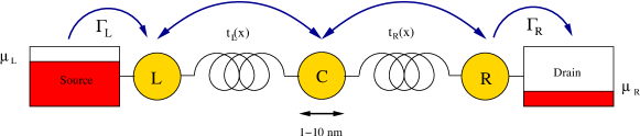
Figure 2.2: Schematic representation of the Triple-dot Shuttle: the leads and the three-dot array are represented. The arrows mimic the electrical dynamics. Single and double arrows indicate that the tunneling from and to the lead is always in a given direction and incoherent while the internal dynamics of the system is subject to coherent oscillations. The mechanical motion of the central dot confined to a harmonic potential is represented by the springs.

Chapter 3 Generalized Master Equation

The state of a physical system is determined by the measurement of a certain number of observables. Repeated measurements of a given observable always return the same expectation value when the system is in an eigenstate for that particular observable. The uncertainty principle ensures us that, for quantum systems, there are incompatible observables that can not be measured at the same time with indefinite precision.

Given a generic quantum system $\mathcal{S}$ and a complete set of compatible observables $\mathcal{A}_{i}$ [25], an eigenstate of the system for all observables is defined by the set of the corresponding expectation values, i.e. the quantum numbers $a_{i}$. Each of the possible sets of expectation values is associated with an eigenvector in the Hilbert space of the system. More precisely the Hilbert space of the system is spanned by the eigenvectors of a complete set of compatible observables.

A pure state of the system is represented by a radius (class of equivalence of normalized vectors with arbitrary phase) of this Hilbert space. We call $|\psi\rangle$ a representative vector of a radius. Observables are associated to Hermitian operators on the Hilbert space of the system. The dynamics of the quantum system is governed by the Hamiltonian operator, i.e. the operator associated to the observable energy. Given an initial vector, the Schrödinger equation prescribes the evolution of this vector at all times:

$$i\hbar\frac{d}{dt}|\psi(t)\rangle=\mathcal{H}|\psi(t)\rangle$$ (3.1)

with the initial condition $|\psi(0)\rangle=|\psi_{0}\rangle$. An equivalent formulation of the dynamics can be given in terms of projector operators $|\psi\rangle\!\langle\psi|$. A projector is independent from the arbitrary phase of the vector $|\psi\rangle$, it is then equivalent to a radius of the Hilbert space and represents a pure state of the system. Using the Leibnitz theorem for derivatives and the Schrödinger equation we derive the equation of Liouville-von Neumann:

$$\frac{d\rho}{dt}=-\frac{i}{\hbar}[\mathcal{H},\rho]$$ (3.2)

where $\rho\equiv|\psi\rangle\!\langle\psi|$, $[A,B]\equiv AB-BA$ is the commutator of the operators $A$ and $B$. The operator $\rho$ is usually called density operator. For each basis of the Hilbert space all the operators have a matrix representation. The matrix that corresponds to the density operator is called density matrix. Each vector of the basis of the Hilbert space corresponds to a particular eigenstate of the system defined by a set of quantum numbers. The diagonal elements of the density matrix are called populations. Each population represents the probability that the system in the pure state $|\psi\rangle\!\langle\psi|$ is in the eigenstate defined by the corresponding set of quantum numbers. The trace of the density matrix is one and supports this probabilistic interpretation. The off-diagonal terms of the density matrix are the coherencies of the system. They reflect the linear structure of the Hilbert space. A linear combination of eigenvectors gives rise to a pure state with non-zero coherencies.

Not all density operators correspond to pure states. A convex linear combination of pure states $|\psi_{n}\rangle\!\langle\psi_{n}|,n=1,...,N$ is called statistical mixture:

$$\rho=\sum_{n=1}^{N}P_{n}|\psi_{n}\rangle\!\langle\psi_{n}|$$ (3.3)

where $P_{n}\in[0,1),\sum_{n}P_{n}=1$. This is an incoherent superposition of pure states. Also statistical mixtures obey the Liuoville-von Neumann equation of motion (3.2).

The master equation is an equation of motion for the populations. It is a coarse grained equation that neglects coherencies. It was derived the first time by Pauli under the assumption that coherencies have random phases in time due to fast molecular dynamics. It reads:

$$\frac{dP_{n}(t)}{dt}=\sum_{m}[\Gamma_{nm}P_{m}(t)-\Gamma_{mn}P_{n}(t)]$$ (3.4)

where $P_{n}$ is the population of the eigenstate $n$ and $\Gamma_{nm}$ is the rate of probability flow from eigenstate $n$ to $m$ [26].

3.1 Coherent dynamics of small open systems

The master equation is usually derived for models in which a“small” system with few degrees of freedom is in interaction with a “large” bath with effectively an infinite number of degrees of freedom. The Liouville von-Neumann equation of motion for the total density matrix is very complicated to solve and actually contains too much information since it also takes into account coherencies of the bath. It is useful to average it over bath variables and obtain an equation of motion for the density matrix of the system (the reduced density matrix). With no further simplification this equation is called Generalized Master Equation (GME) since it involves not only the populations but also the coherencies of the small subsystem. The derivation of the GME from the equation of Liouville-von Neumann is far from trivial and also non-universal: it involves a series of approximations justified by the physical properties of the model at hand. Despite the apparent similarities, the two equations are deeply different: the equation of Liouville-von Neumann describes the reversible dynamics of a closed system; the GME, instead, describes the irreversible dynamics of an open system that continuously exchange energy with the bath.

Shuttle devices are small systems coupled to different baths (leads, thermal bath) but they maintain a high degree of correlation between electrical and mechanical degrees of freedom captured by the coherencies of the reduced density matrix. The GME seems to be a good candidate for the description of their dynamics.

In the next two sections we will derive two GMEs using two different approaches. They are both necessary for the description of the shuttling devices since they correspond to the different coupling of the system to the mechanical and electrical baths.

3.2 Quantum optical derivation

The harmonic oscillator weakly coupled to a bosonic bath is a typical problem analyzed in quantum optics. This model well describes in shuttling devices the interaction of the mechanical degree of freedom of the NEMS with its environment. Following section $5.1$ of the book “Quantum Noise” by C. W. Gardiner and P. Zoller [27] we start considering a small system S coupled to a large bath B described by the generic Hamiltonian:

$$H=H_{\rm S}+H_{\rm B}+H_{\rm I}$$ (3.5)

where $H_{\rm S}$ and $H_{\rm B}$ respectively describe the dynamics of the decoupled system and bath and $H_{\rm I}$ represents the interaction between the two that we assume weak. The density operator $\rho$ (the state of the system$+$bath) satisfies, in the Schrödinger picture, the equation of Liouville-von Neumann:

$$\dot{\rho}=-\frac{i}{\hbar}[H_{\rm S}+H_{\rm B}+H_{\rm I},\rho]$$ (3.6)

The state of the system is described by the reduced density matrix $\sigma$:

$$\sigma={\rm Tr}_{\rm B}\{\rho\}$$ (3.7)

where ${\rm Tr}_{\rm B}$ indicates the partial trace over the bath degrees of freedom. Our task is to derive from (3.6) an equation of motion for the reduced density matrix $\sigma$.

3.2.1 Interaction picture

We start by going to the interaction picture and we use as non-interacting Hamiltonian $H_{\rm S}+H_{\rm B}$. We indicate all the operators in the interaction picture with a tilde. The total density operator in the interaction picture reads:

$$\tilde{\rho}(t)=\exp\left[\frac{i}{\hbar}(H_{\rm S}+H_{\rm B})t\right]\rho(t)\exp\left[-\frac{i}{\hbar}(H_{\rm S}+H_{\rm B})t\right]$$ (3.8)

and obeys the equation of motion:

$$\dot{\tilde{\rho}}(t)=-\frac{i}{\hbar}[\tilde{H}_{\rm I}(t),\tilde{\rho}(t)]$$ (3.9)

where

$$\tilde{H}_{\rm I}(t)=\exp\left[\frac{i}{\hbar}(H_{\rm S}+H_{\rm B})t\right]H_{\rm I}\exp\left[-\frac{i}{\hbar}(H_{\rm S}+H_{\rm B})t\right]$$ (3.10)

From (3.7) and (3.8) it follows that

$$\sigma(t)={\rm Tr}_{\rm B}\left\{\exp\left[-\frac{i}{\hbar}(H_{\rm S}+H_{\rm B})t\right]\tilde{\rho}(t)\exp\left[\frac{i}{\hbar}(H_{\rm S}+H_{\rm B})t\right]\right\}$$ (3.11)

The exponentials of $H_{\rm B}$ can be cancelled using the cyclic property of the trace since $H_{\rm B}$ depends only on bath variables. We get

$$\sigma(t)=\exp\left[-\frac{i}{\hbar}H_{\rm S}t\right]\tilde{\sigma}(t)\exp\left[\frac{i}{\hbar}H_{\rm S}t\right]$$ (3.12)

where

$$\tilde{\sigma}(t)\equiv{\rm Tr}_{B}\{\tilde{\rho}(t)\}$$ (3.13)

In other terms the interaction picture for the reduced density matrix is effectively obtained only from the non-interacting Hamiltonian for the system $H_{\rm S}$.

3.2.2 Initial conditions

We assume that the system and the bath are initially independent, the initial total density operator $\rho$ is then factorized into the tensor product:

$$\rho(0)=\sigma(0)\otimes\rho_{\rm B}$$ (3.14)

For definiteness we assume the bath to be in thermal equilibrium:

$$\rho_{\rm B}=\frac{e^{-\beta H_{\rm B}}}{{\rm Tr_{B}}e^{-\beta H_{\rm B}}}$$ (3.15)

where $\beta=1/k_{B}T$ is the inverse temperature.

3.2.3 Reformulation of the equation of motion

It is most important for the derivation of the GME to recast the original equation of motion in the interaction picture (3.9) into an integro-differential form. The integral from $0$ to $t$ of (3.9) reads

$$\tilde{\rho}(t)=\tilde{\rho}(0)-\frac{i}{\hbar}\int_{0}^{t}dt^{\prime}[\tilde{H}_{\rm I}(t^{\prime}),\tilde{\rho}(t^{\prime})]$$ (3.16)

and inserted back into (3.9) itself gives

$$\dot{\tilde{\rho}}(t)=-\frac{i}{\hbar}[\tilde{H}_{\rm I}(t),\tilde{\rho}(0)]-\frac{1}{\hbar^{2}}\int_{0}^{t}dt^{\prime}\tilde{H}_{\rm I}(t),[\tilde{H}_{\rm I}(t^{\prime}),\tilde{\rho}(t^{\prime})]]$$ (3.17)

3.2.4 Average over the bath variables

We take the partial trace over the bath variables on both sides of (3.17). From the definition of the reduced density operator (3.7) we obtain, for the LHS, $\dot{\tilde{\sigma}}$. We assume that the first term in the RHS vanishes, namely

$${\rm Tr_{B}}[\tilde{H}_{\rm I},\tilde{\rho}(0)]=0$$ (3.18)

where $\tilde{\rho}(0)=\rho(0)=\sigma(0)\otimes\rho_{\rm B}$. This means that the interaction Hamiltonian has a bath component with zero average. It is not difficult to fulfill this condition in general by a redefinition of the system and interaction Hamiltonian that subtracts the average of the bath component from the latter.

3.2.5 Weak coupling

We assume that $H_{\rm I}$ is only a small perturbation of $H_{\rm S}$ and $H_{\rm B}$. This condition allows a factorization at all times of the total density operator into its system and bath components. The density operator of the bath is also taken as constant in time:

$$\tilde{\rho}(t)\approx\tilde{\sigma}(t)\otimes\rho_{\rm B}$$ (3.19)

The factorization assumption can be weakened. We introduce for this purpose the notion of correlation function. Given a physical system in the state described by the stationary density operator $\rho$ and two operators $\tilde{O_{\rm 1}}$ and $\tilde{O_{\rm 2}}$ the correlation function between $\tilde{O_{\rm 1}}$ and $\tilde{O_{\rm 2}}$ in this order and at times $t$ and $t^{\prime}$ is:

$$C_{O_{1}O_{2}}(t,t^{\prime})\equiv{\rm Tr}\{\rho\tilde{O_{\rm 1}}(t)\tilde{O_{\rm 2}}(t^{\prime})\}$$ (3.20)

where the trace is taken over the the Hilbert space of the system and the operators are in Heisenberg picture. Returning to our system-bath model, we assume that the interaction Hamiltonian is a sum of operators in the form $F_{\rm S}A_{\rm B}$. The minimal requirement for the weak coupling approximation is that the correlation functions of the bath are not influenced by the state of the system. In formulas:

$${\rm Tr_{B}}\{[\tilde{A_{\rm B}}(t),[\tilde{A_{\rm B}}(t^{\prime}),\tilde{\rho}(t^{\prime})]]\}\approx\tilde{\sigma}(t^{\prime})\otimes{\rm Tr_{B}}\{[\tilde{A_{\rm B}}(t),[\tilde{A_{\rm B}}(t^{\prime}),\rho_{\rm B}]]\}$$ (3.21)

3.2.6 Markov approximation

The integro-differential equation for $\tilde{\sigma}$ obtained in the weak coupling approximation is non-local in time. The state of the system at time $t$ depends on the history of the model starting from the initial time $t=0$. This is the meaning of the integral on the RHS of the equation

$$\dot{\tilde{\sigma}}=-\frac{1}{\hbar^{2}}\int_{0}^{t}dt^{\prime}{\rm Tr_{B}}\{[\tilde{H_{\rm I}}(t),[\tilde{H_{\rm I}}(t^{\prime}),\tilde{\sigma}(t^{\prime})\otimes\rho_{\rm B}]]\}.$$ (3.22)

obtained from (3.21) by tracing over bath variables. Due to the different sizes and the weak coupling the effects on the bath of the interaction with the system are negligible. The bath is a classical macroscopic object in thermal equilibrium. Its stationary state is a thermal state: an incoherent statistical mixture of energy eigenstates. The coherencies in the bath introduced by the interaction with the system decay on a time scale called the correlation time. This is precisely the decaying time of the correlation functions of the bath. If the correlation time of the bath is much shorter than the typical time scale for the system dynamics, then we can make in (3.21) the replacement:

$$\tilde{\sigma}(t^{\prime})\to\tilde{\sigma}(t)$$ (3.23)

and obtain in this way a differential equation for $\tilde{\sigma}$. Finally, if we are interested in the dynamics of the system for times much longer than the bath correlation time, the lower integration limit in (3.21) can be moved to $-\infty$ since the initial bath correlation are irrelevant. With this set of approximations the knowledge of the state of the system at some time $t_{0}$ is enough to determine the state at all times $t>t_{0}$. This property is called Markov property. In the weak coupling limit and assuming short correlation times in the heat bath we have derived the following GME for the reduced density operator in the interaction picture:

$$\dot{\tilde{\sigma}}=-\frac{1}{\hbar^{2}}\int_{0}^{\infty}d\tau{\rm Tr_{B}}\{[\tilde{H}_{\rm I}(t),[\tilde{H}_{\rm I}(t-\tau),\tilde{\sigma}(t)\otimes\rho_{\rm B}]]\}$$ (3.24)

To proceed further the precise knowledge of the model Hamiltonian is required. In section 3.4 we will specialize this derivation of the GME to the description of the dissipative environment of the shuttling devices.

3.3 Derivation “à la Gurvitz”

The tunneling coupling of the shuttling devices to their electrical baths (the leads) is not weak. It sets, on the contrary, the time scale of the electrical dynamics that in the shuttling regime is comparable with the period of the mechanical oscillations in the system.

In the SDQS the tunneling amplitudes depend exponentially on the displacement of the central dot from the equilibrium position. The oscillations of the QD modify correspondingly the tunneling rates. In the shuttling regime the following non-adiabatic condition is fulfilled:

$$\bar{\Gamma}_{\rm L,R}=\frac{\omega}{2\pi}$$ (3.25)

where the average can be interpreted as a classical average over the stable limit cycle trajectory or quantum mechanically as an expectation value in the stationary state. In both cases Coulomb blockade must be taken into account for a correct evaluation of the average rate.

In the TDQS the coupling to the leads is constant and represents a tunable parameter of the model. Also for this device the cleanest shuttling regime is achieved for a rather high coupling (and associated tunneling rates comparable with the mechanical frequency).

In 1996 S. Gurvitz and Ya. S. Prager proposed a microscopic derivation of the GME for quantum transport with an arbitrary coupling to the leads [28]. Following their article we give now in detail the derivation of the rate equations for transport of non-interacting spin-less particles through a static single dot connected to leads. Even if in this oversimplified case the result is intuitive and could be guessed just using common sense, the generic features of the derivation will appear. We extend the result to particles with spin in strong Coulomb blockade and eventually we conclude the section showing that also coherent transport can be treated in this formalism and we derive the GME for a static double dot device.

Let us consider a quantum dot connected to two electronic leads. We neglect (at the moment) the spin degree of freedom and Coulomb interaction between the electrons. The energy levels in the macroscopic leads are very dense while they are discrete in the microscopic QD. We assume that only one level in the dot participates in the dynamics of the model.

3.3.1 Many-body basis expansion

The Hamiltonian for the model reads

$$\begin{split}H=&\sum_{l}\varepsilon_{l}c_{l}^{\dagger}c_{l}^{\phantom{\dagger}}+\varepsilon_{1}c_{1}^{\dagger}c_{1}^{\phantom{\dagger}}+\sum_{r}\varepsilon_{r}c_{r}^{\dagger}c_{r}^{\phantom{\dagger}}\\ &+\sum_{l}\Omega_{l}(c_{l}^{\dagger}c_{1}^{\phantom{\dagger}}+c_{1}^{\dagger}c_{l}^{\phantom{\dagger}})+\sum_{r}\Omega_{r}(c_{r}^{\dagger}c_{1}^{\phantom{\dagger}}+c_{1}^{\dagger}c_{r}^{\phantom{\dagger}})\end{split}$$ (3.26)

where $c_{l}^{\dagger},c_{1}^{\dagger},c_{r}^{\dagger}$ create a particle in the left lead (energy level $\varepsilon_{l}$), in the dot and in the right lead (energy level $\varepsilon_{r}$) respectively. $\varepsilon_{1}$ is the energy level of the dot and $\Omega_{l\,(r)}$ the tunneling amplitudes between the dot and the left (right) lead. For temperatures much smaller than the Fermi energy of the leads we can approximate their Fermi distributions by step functions. The chemical potential of the left (right) lead is assumed much higher (lower) than the dot energy level.

We identify the empty state $|0\rangle$ for the model with the condition of empty dot and leads filled up to their Fermi energies. Then we gradually move electrons from the emitter to the dot and finally to the collector and associate a new vector to each state of this “decaying chain”. We construct in this way an infinite many-body basis that defines the Hilbert space for the model. The first few elements of the basis read:

$$|0\rangle\qquad c_{1}^{\dagger}c_{l_{1}}^{\phantom{\dagger}}|0\rangle\qquad c_{r_{1}}^{\dagger}c_{l_{1}}^{\phantom{\dagger}}|0\rangle\qquad c_{1}^{\dagger}c_{r_{1}}^{\dagger}c_{l_{1}}^{\phantom{\dagger}}c_{l_{2}}^{\phantom{\dagger}}|0\rangle\qquad c_{r_{2}}^{\dagger}c_{r_{1}}^{\dagger}c_{l_{1}}^{\phantom{\dagger}}c_{l_{2}}^{\phantom{\dagger}}|0\rangle\,\ldots$$ (3.27)

where we choose by convention to move all the creation operators to the left and the annihilation operators to the right. We also assume with the two groups that $\varepsilon_{l_{i}}<\varepsilon_{l_{i+1}}$ and $\varepsilon_{r_{i}}<\varepsilon_{r_{i+1}}$ to avoid double counting.

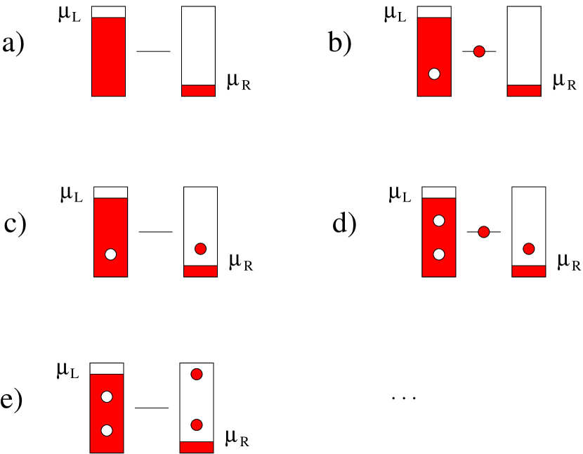
Figure 3.1: Schematic representation of the first elements of the many-body basis for the single dot model. Electrons are progressively taken from the emitter and moved to the QD and finally to the collector. The vectors represented are in the order ${\rm a)}=|0\rangle$, ${\rm b)}=c_{1}^{\dagger}c_{l_{1}}|0\rangle$, ${\rm c)}=c_{r_{1}}^{\dagger}c_{l_{1}}|0\rangle$, ${\rm d)}=c_{1}^{\dagger}c_{r_{1}}^{\dagger}c_{l_{1}}c_{l_{2}}|0\rangle$, ${\rm e)}=c_{r_{2}}^{\dagger}c_{r_{1}}^{\dagger}c_{l_{1}}c_{l_{2}}|0\rangle$.

The state of the model is described by the many-particle vector $|\Psi(t)\rangle$ which we can expand over the basis:

$$\begin{split}|\Psi(t)\rangle=&\Big{[}b_{0}(t)+\sum_{l_{1}}b_{1l_{1}}(t)c_{1}^{\dagger}c_{l_{1}}^{\phantom{\dagger}}+\sum_{l_{1},r_{1}}b_{l_{1}r_{1}}(t)c_{r_{1}}^{\dagger}c_{l_{1}}^{\phantom{\dagger}}\\ &+\!\sum_{l_{1}<l_{2},r_{1}}b_{1l_{1}l_{2}r_{1}}(t)c_{1}^{\dagger}c_{r_{1}}^{\dagger}c_{l_{1}}^{\phantom{\dagger}}c_{l_{2}}^{\phantom{\dagger}}+\!\sum_{l_{1}<l_{2},r_{1}<r_{2}}b_{l_{1}l_{2}r_{1}r_{2}}(t)c_{r_{2}}^{\dagger}c_{r_{1}}^{\dagger}c_{l_{1}}^{\phantom{\dagger}}c_{l_{2}}^{\phantom{\dagger}}+\ldots\Big{]}|0\rangle\end{split}$$ (3.28)

3.3.2 Recursive equation of motion for the coefficients

The vector $|\Psi(t)\rangle$ obeys the Schrödinger equation $i\hbar|\dot{\Psi}(t)\rangle=H|\Psi(t)\rangle$ and we impose the initial condition $|\Psi(0)\rangle=|0\rangle$. In terms of the coefficients of the expansion (3.28) we obtain an infinite set of differential equations with the initial condition $b_{0}(0)=1$ and all the other coefficients equal to $0$ at time $t=0$.

Due to the quadratic form of the Hamiltonian, the infinite set of differential equations for the coefficients $b$’s presents a recursive structure: each coefficient is linked in its equation of motion only to the previous and the next in the “decaying chain”(3.28). Since we are interested in keeping track of the state of the dot we condense the full system of equations into two equations for the generic coefficients $b_{\{l_{j}\}_{j=1}^{n}\{r_{j}\}_{j=1}^{n}}(t)$ and $b_{1\{l_{j}\}_{j=1}^{n+1}\{r_{j}\}_{j=1}^{n}}(t)$:

$$\begin{split}i\dot{b}_{\{l_{j}\}_{j=1}^{n}\{r_{j}\}_{j=1}^{n}}=&\left[\sum_{k=1}^{n}(\varepsilon_{r_{k}}-\varepsilon_{l_{k}})\right]b_{\{l_{j}\}_{j=1}^{n}\{r_{j}\}_{j=1}^{n}}\\ &\!\!\!\!+\sum_{l_{n+1}}\Omega_{l_{n+1}}b_{1\{l_{j}\}_{j=1}^{n+1}\{r_{j}\}_{j=1}^{n}}+\sum_{k=1}^{n}(-1)^{k-n}\Omega_{r_{k}}b_{1\{l_{j}\}_{j=1}^{n}\{r_{j}\}_{j=1}^{n}\backslash\{r_{k}\}}\\ i\dot{b}_{1\{l_{j}\}_{j=1}^{n+1}\{r_{j}\}_{j=1}^{n}}=&\left[\varepsilon_{1}+\sum_{k=1}^{n}(\varepsilon_{r_{k}}-\varepsilon_{l_{k}})-\varepsilon_{l_{n+1}}\right]b_{1\{l_{j}\}_{j=1}^{n+1}\{r_{j}\}_{j=1}^{n}}\\ &\!\!\!\!+\sum_{r_{n+1}}\Omega_{r_{n+1}}b_{\{l_{j}\}_{j=1}^{n+1}\{r_{j}\}_{j=1}^{n+1}}+\sum_{k=1}^{n+1}(-1)^{k-n-1}\Omega_{l_{k}}b_{\{l_{j}\}_{j=1}^{n+1}\backslash\{l_{k}\}\{r_{j}\}_{j=1}^{n}}\\ \end{split}$$ (3.29)

where $\hbar=1$ and the sums over labels (e.g. $\sum_{l_{n+1}}$) are continuous sums over all the possible energy levels of the leads. We also used the shortened notations:

$$\begin{split}b_{\{l_{j}\}_{j=1}^{n}\{r_{j}\}_{j=1}^{n}}&\equiv b_{l_{1}l_{2}l_{3}\ldots l_{n}r_{1}r_{2}r_{3}\ldots r_{n}}(t)\\ b_{1\{l_{j}\}_{j=1}^{n+1}\backslash\{l_{k}\}\{r_{j}\}_{j=1}^{n}}&\equiv b_{1l_{1}l_{2}l_{3}\ldots l_{k-1}l_{k+1}\ldots l_{n+1}r_{1}r_{2}r_{3}\ldots r_{n}}(t)\end{split}$$ (3.30)

In order to proceed in the derivation of the rate equations it is most convenient to make the Laplace transform of the system of differential equations (3.29). We obtain the system of algebraic equations:

$$\begin{split}&\left[E+\sum_{k=1}^{n}(\varepsilon_{l_{k}}-\varepsilon_{r_{k}})\right]\tilde{b}_{\{l_{j}\}_{j=1}^{n}\{r_{j}\}_{j=1}^{n}}(E)\\ &-\sum_{l_{n+1}}\Omega_{l_{n+1}}\tilde{b}_{1\{l_{j}\}_{j=1}^{n+1}\{r_{j}\}_{j=1}^{n}}(E)-\sum_{k=1}^{n}(-1)^{k-n}\Omega_{r_{k}}\tilde{b}_{1\{l_{j}\}_{j=1}^{n}\{r_{j}\}_{j=1}^{n}\backslash\{r_{k}\}}(E)=i\delta_{n0}\\ &\left[E-\varepsilon_{1}+\sum_{k=1}^{n}(\varepsilon_{l_{k}}-\varepsilon_{r_{k}})+\varepsilon_{l_{n+1}}\right]\tilde{b}_{1\{l_{j}\}_{j=1}^{n+1}\{r_{j}\}_{j=1}^{n}}(E)\\ &-\sum_{r_{n+1}}\Omega_{r_{n+1}}\tilde{b}_{\{l_{j}\}_{j=1}^{n+1}\{r_{j}\}_{j=1}^{n+1}}(E)-\sum_{k=1}^{n+1}(-1)^{k-n-1}\Omega_{l_{k}}\tilde{b}_{\{l_{j}\}_{j=1}^{n+1}\backslash\{l_{k}\}\{r_{j}\}_{j=1}^{n}}(E)=0\\ \end{split}$$ (3.31)

where the Laplace transformed coefficients are indicated with a tilde and are functions of the variable $E$ (that we assume to have an imaginary part to ensure convergence of the Laplace integral). At this level the left-right asymmetry reveals itself in the number of “decay channels”. Each state of the chain (3.27) is coupled to an infinite number of right states and only a finite number of left states. Since the couplings are equivalent this results in a statistically definite direction of motion for the electrons.

3.3.3 Injection and ejection rates

The continuous sums in (3.31) can be simplified using the recursive structure of the equation of motion. We isolate in the second equation of (3.31) the coefficient $\tilde{b}_{1\{l_{j}\}_{j=1}^{n+1}\{r_{j}\}_{j=1}^{n}}(E)$ and insert the result into the first equation of (3.31). The continuous sum results into two terms:

$$\sum_{l_{n+1}}\sum_{r_{n+1}}\frac{\Omega_{l_{n+1}}\Omega_{r_{n+1}}}{E-\varepsilon_{1}+\sum_{k=1}^{n}(\varepsilon_{l_{k}}-\varepsilon_{r_{k}})+\varepsilon_{l_{n+1}}}\tilde{b}_{\{l_{j}\}_{j=1}^{n+1}\{r_{j}\}_{j=1}^{n+1}}$$ (3.32)

and

$$\sum_{l_{n+1}}\sum_{k=1}^{n+1}(-1)^{k-n-1}\frac{\Omega_{l_{n+1}}\Omega_{l_{k}}}{E-\varepsilon_{1}+\sum_{i=1}^{n}(\varepsilon_{l_{i}}-\varepsilon_{r_{i}})+\varepsilon_{l_{n+1}}}\tilde{b}_{\{l_{j}\}_{j=1}^{n+1}\backslash\{l_{k}\}\{r_{j}\}_{j=1}^{n}}$$ (3.33)

Since the energy levels in the leads are dense we can substitute

$$\sum_{l_{n+1}}\to\int_{-\infty}^{+\infty}d\varepsilon_{l_{n+1}}D_{L}(\varepsilon_{l_{n+1}})$$ (3.34)

where $D(\varepsilon_{l_{n+1}})$ is the density of states in the left lead calculated at energy $\varepsilon_{l_{n+1}}$ and we have extended the integration limits to infinity in the wide band and high bias approximation. We can evaluate now the sum over $l_{n+1}$ in (3.32) and (3.33) using residues method. Since all the poles are in the same half plane we can neglect all terms which are asymptotically $o(|\varepsilon_{l_{n+1}}|^{-1})$ for $|\varepsilon_{l_{n+1}}|\to\infty$. It is clear from the algebraic system (3.31) that a coefficient $\tilde{b}$ that has among its indices $\varepsilon_{l_{n+1}}$ behaves asymptotically at least like $|\varepsilon_{l_{n+1}}|^{-1}$. For this reason (3.32) vanishes and only one term is left from (3.33):

$$\tilde{b}_{\{l_{j}\}_{j=1}^{n}\{r_{j}\}_{j=1}^{n}}\int_{-\infty}^{+\infty}d\varepsilon_{l+1}D_{L}(\varepsilon_{l_{n+1}})\frac{\Omega_{l_{n+1}}^{2}}{E-\varepsilon_{1}+\sum_{i=1}^{n}(\varepsilon_{l_{i}}-\varepsilon_{r_{i}})+\varepsilon_{l_{n+1}}}$$ (3.35)

For the evaluation of the integral is enough that the tunneling amplitude $\Omega_{l_{n+1}}$ and the density of states $D_{L}(\varepsilon_{l_{n+1}})$ are analytical and non-zero where the denominator vanishes. We assume that they are constant to avoid $n$-dependence in the tunneling rates and perform the integral in (3.35). The second equation (3.31) can be treated analogously and the system reads:

$$\begin{split}&\left[E+\sum_{k=1}^{n}(\varepsilon_{l_{k}}-\varepsilon_{r_{k}})+i\frac{\Gamma_{L}}{2}\right]\tilde{b}_{\{l_{j}\}_{j=1}^{n}\{r_{j}\}_{j=1}^{n}}(E)\\ &\phantom{aaaaa}-\sum_{k=1}^{n}(-1)^{k-n}\Omega_{r_{k}}\tilde{b}_{1\{l_{j}\}_{j=1}^{n}\{r_{j}\}_{j=1}^{n}\backslash\{r_{k}\}}(E)=i\delta_{n0}\\ &\left[E-\varepsilon_{1}+\sum_{k=1}^{n}(\varepsilon_{l_{k}}-\varepsilon_{r_{k}})+\varepsilon_{l_{n+1}}+i\frac{\Gamma_{R}}{2}\right]\tilde{b}_{1\{l_{j}\}_{j=1}^{n+1}\{r_{j}\}_{j=1}^{n}}(E)\\ &\phantom{aaaaa}-\sum_{k=1}^{n+1}(-1)^{k-n-1}\Omega_{l_{k}}\tilde{b}_{\{l_{j}\}_{j=1}^{n+1}\backslash\{l_{k}\}\{r_{j}\}_{j=1}^{n}}(E)=0\\ \end{split}$$ (3.36)

where we have introduced the injection and ejection rates $\Gamma_{L}$ and $\Gamma_{R}$

$$\begin{split}\Gamma_{L}&\equiv 2\pi D_{L}\Omega_{L}^{2}\\ \Gamma_{R}&\equiv 2\pi D_{R}\Omega_{R}^{2}\end{split}$$ (3.37)

whith the energy independent tunneling amplitudes ($\Omega_{L}$ and $\Omega_{R}$) and density of states ($D_{L}$ and $D_{R}$).

3.3.4 The reduced density matrix

The reduced density operator is defined as the trace over the bath variables of the total density operator:

$$\sigma(t)={\rm Tr}_{B}\{|\Psi(t)\rangle\!\langle\Psi(t)|\}$$ (3.38)

The matrix elements of the reduced density operators are explicitly

$$\sigma_{ij}(t)=\sum_{\{B\}}\langle i_{S},B|\Psi(t)\rangle\!\langle\Psi(t)|B,j_{S}\rangle$$ (3.39)

where $|i_{S},B\rangle,i=0,1$ is the vector that corresponds to the empty or charged dot (the system) and a particular configuration $B$ of the leads (the baths). We assume that the bath state $B$ does not contain coherent superpositions of states with different number of particles. This implies the vanishing of coherencies in the reduced density matrix. It is useful to organize the sum over the bath configurations according to the number of extra electrons (holes) collected into the right (left) lead.

$$\sigma_{ii}(t)=\sum_{n=0}^{\infty}\sum_{\{B_{n}\}}\langle i_{S},B_{n}|\Psi(t)\rangle\!\langle\Psi(t)|B_{n},i_{S}\rangle=\sum_{n=0}^{\infty}\sigma_{ii}^{(n)}(t)$$ (3.40)

where $B_{n}$ is a configuration of the baths with $n$ extra electrons in the collector and we have introduced the n-resolved density matrix $\sigma^{(n)}$. Using the expansion of the vector $|\Psi(t)\rangle$ in the many-body basis (3.27) we can express the $n$-resolved density matrix in terms of the coefficients $b$. For the two non-vanishing elements:

$$\begin{split}\sigma_{00}^{(n)}&=\sum_{\{B_{n}\}}|\langle 0_{S},B_{n}|\Psi(t)\rangle|^{2}=\sum_{\{l_{k}\}\{r_{k}\}}|b_{\{l_{k}\}_{k=1}^{n}\{r_{k}\}_{k=1}^{n}}(t)|^{2}\\ \sigma_{11}^{(n)}&=\sum_{\{B_{n}\}}|\langle 1_{S},B_{n}|\Psi(t)\rangle|^{2}=\sum_{\{l_{k}\}\{r_{k}\}}|b_{1\{l_{k}\}_{k=1}^{n+1}\{r_{k}\}_{k=1}^{n}}(t)|^{2}\end{split}$$ (3.41)

where the sums are calculated over all the possible configurations of indistinguishable particles (e.g. $\sum_{\{l_{k}\}}\equiv\sum_{l_{1}<l_{2}<l_{3}<\ldots<l_{n}}$). The time-dependent matrix elements of the reduced density matrix are connected to the coefficients $\tilde{b}(E)$ by the inverse of the Laplace transform:

$$\begin{split}\sigma^{(n)}_{00}(t)&=\sum_{\{l_{k}\}\{r_{k}\}}\int\frac{dEdE^{\prime}}{4\pi^{2}}\tilde{b}_{\{l_{k}\}_{k=1}^{n}\{r_{k}\}_{k=1}^{n}}(E)\tilde{b}^{*}_{\{l_{k}\}_{k=1}^{n}\{r_{k}\}_{k=1}^{n}}(E^{\prime})e^{i(E-E^{\prime})t}\\ \sigma^{(n)}_{11}(t)&=\sum_{\{l_{k}\}\{r_{k}\}}\int\frac{dEdE^{\prime}}{4\pi^{2}}\tilde{b}_{1\{l_{k}\}_{k=1}^{n+1}\{r_{k}\}_{k=1}^{n}}(E)\tilde{b}^{*}_{1\{l_{k}\}_{k=1}^{n+1}\{r_{k}\}_{k=1}^{n}}(E^{\prime})e^{i(E-E^{\prime})t}\\ \end{split}$$ (3.42)

Apart from being a natural step in the derivation of the GME in the Gurvitz approach, the $n$-resolved density matrix contains the additional information on the number of electrons collected in the resevoir at time $t$. This information is very useful to the calculation of the current noise in the SDQS where the quantum regression theorem can not be applied due to the form of the current operator that involves both system and bath operators.

3.3.5 Generalized Master Equation

The equation of motion for the reduced density matrix is obtained combining (3.42) and (3.36). First we derive an equation of motion for the $n$-resolved reduced density matrix $\sigma^{(n)}$. The case of the empty dot population with $n=0$ is special due to the particular choice of the initial condition and we treat it separately. The starting point is the first of the equations (3.36) specialized for $n=0$, namely:

$$\left(E+i\frac{\Gamma_{L}}{2}\right)\tilde{b}_{0}(E)=i$$ (3.43)

We taking the inverse Laplace transform and obtain

$$\dot{b}_{0}(t)=-\frac{\Gamma_{L}}{2}b_{0}(t)$$ (3.44)

The definition of $\sigma_{00}^{(0)}$ and the Leibnitz theorem for derivatives lead to the conclusion:

$$\dot{\sigma}_{00}^{(0)}=\dot{b}_{0}b_{0}^{*}+b_{0}\dot{b}_{0}^{*}=-\Gamma_{L}b_{0}b_{0}^{*}=-\Gamma_{L}\sigma_{00}^{(0)}$$ (3.45)

This argument is applied also in the case with $n\neq 0$ but the structure of the equation is more complex and in general a final continuous sum must be evaluated. We take the first equation in (3.36) and multiply it by $\tilde{b}^{*}_{\{l_{j}\}_{j=1}^{n}\{r_{j}\}_{j=1}^{n}}(E^{\prime})$$e^{-i(E-E^{\prime})t}$. Then we subtract side by side the complex conjugate of the first equation of (3.36) evaluated in $E^{\prime}$ and multiplied by $\tilde{b}_{\{l_{j}\}_{j=1}^{n}\{r_{j}\}_{j=1}^{n}}(E)$$e^{-i(E-E^{\prime})t}$. Finally we integrate in $dE$ and $dE^{\prime}$ and sum over the bath configurations with $n$ electrons in the collector. We repeat the procedure also for the second equation in (3.36) and obtain:

$$\begin{split}&\sum_{\{l_{j}\}\{r_{j}\}}\!\int\frac{dEdE^{\prime}}{4\pi^{2}}\Big{[}(E-E^{\prime}+i\Gamma_{L})\tilde{b}_{\{l_{j}\}_{j=1}^{n}\{r_{j}\}_{j=1}^{n}}(E)\tilde{b}^{*}_{\{l_{j}\}_{j=1}^{n}\{r_{j}\}_{j=1}^{n}}\!(E^{\prime})e^{-i(E-E^{\prime})t}\\ &-2\Im\Big{(}\sum_{k=1}^{n}(-1)^{k-n}\Omega_{r_{k}}\tilde{b}_{1\{l_{j}\}_{j=1}^{n}\{r_{j}\}_{j=1}^{n}\backslash\{r_{k}\}}(E)\tilde{b}^{*}_{\{l_{j}\}_{j=1}^{n}\{r_{j}\}_{j=1}^{n}}(E^{\prime})e^{-i(E-E^{\prime})t}\Big{)}\Big{]}=0\end{split}$$ (3.46)

for the first equation and similarly

$$\begin{split}&\sum_{\{l_{j}\}\{r_{j}\}}\!\int\frac{dEdE^{\prime}}{4\pi^{2}}\Big{[}(E-E^{\prime}+i\Gamma_{R})\tilde{b}_{1\{l_{j}\}_{j=1}^{n+1}\{r_{j}\}_{j=1}^{n}}(E)\tilde{b}^{*}_{1\{l_{j}\}_{j=1}^{n+1}\{r_{j}\}_{j=1}^{n}}\!(E^{\prime})e^{-i(E-E^{\prime})t}\\ &-2\Im\Big{(}\sum_{k=1}^{n+1}(-1)^{k-n-1}\Omega_{l_{k}}\tilde{b}_{\{l_{j}\}_{j=1}^{n+1}\backslash\{l_{k}\}\{r_{j}\}_{j=1}^{n}}(E)\tilde{b}^{*}_{1\{l_{j}\}_{j=1}^{n+1}\{r_{j}\}_{j=1}^{n}}(E^{\prime})e^{-i(E-E^{\prime})t}\Big{)}\Big{]}=0\\ \end{split}$$ (3.47)

for the second. $\Im$ indicates the imaginary part. In the definition of the $n$-resolved reduced density matrix the two coefficients $b$ correspond to the same bath configuration. The finite sums in equations (3.46) and (3.47) still have coefficients with different bath configuration. Using properties of the Laplace transform, the definition of $\sigma^{(n)}$ and the relations

$$\begin{split}\tilde{b}^{*}_{\{l_{j}\}_{j=1}^{n}\{r_{j}\}_{j=1}^{n}}(E^{\prime})&=\frac{\sum_{k=1}^{n}(-1)^{k-n}\Omega_{r_{k}}\tilde{b}^{*}_{1\{l_{j}\}_{j=1}^{n}\{r_{j}\}_{j=1}^{n}\backslash\{r_{k}\}}(E^{\prime})}{E^{\prime}+\sum_{k=1}^{n}(\varepsilon_{l_{k}}-\varepsilon_{r_{k}})-i\frac{\Gamma_{L}}{2}}\\ \tilde{b}^{*}_{1\{l_{j}\}_{j=1}^{n+1}\{r_{j}\}_{j=1}^{n}}(E^{\prime})&=\frac{\sum_{k=1}^{n+1}(-1)^{k-n-1}\Omega_{l_{k}}\tilde{b}^{*}_{\{l_{j}\}_{j=1}^{n+1}\backslash\{l_{k}\}\{r_{j}\}_{j=1}^{n}}(E^{\prime})}{E^{\prime}-\varepsilon_{1}+\sum_{k=1}^{n}(\varepsilon_{l_{k}}-\varepsilon_{r_{k}})+\varepsilon_{l_{n+1}}-i\frac{\Gamma_{R}}{2}}\end{split}$$ (3.48)

obtained from (3.36), we transform (3.46) and (3.47) into:

$$\begin{split}i(\dot{\sigma}_{00}^{(n)}+\Gamma_{L}\sigma_{00}^{(n)})=\phantom{\Big{[}2\Im\Big{(}\sum_{k,k^{\prime}=1}^{n}\frac{(-1)^{k+k^{\prime}}\Omega_{r_{k}}\Omega_{r_{k^{\prime}}}}{E^{\prime}+\sum_{k=1}^{n}(\varepsilon_{l_{k}}-\varepsilon_{r_{k}})-i\frac{\Gamma_{L}}{2}}}&\\ \sum_{\{l_{j}\}\{r_{j}\}}\int\frac{dEdE^{\prime}}{4\pi^{2}}\Big{[}2\Im\Big{(}\sum_{k,k^{\prime}=1}^{n}\frac{(-1)^{k+k^{\prime}}\Omega_{r_{k}}\Omega_{r_{k^{\prime}}}}{E^{\prime}+\sum_{k=1}^{n}(\varepsilon_{l_{k}}-\varepsilon_{r_{k}})-i\frac{\Gamma_{L}}{2}}&\\ \tilde{b}_{1\{l_{j}\}_{j=1}^{n}\{r_{j}\}_{j=1}^{n}\backslash\{r_{k}\}}(E)\tilde{b}^{*}_{1\{l_{j}\}_{j=1}^{n}\{r_{j}\}_{j=1}^{n}\backslash\{r_{k^{\prime}}\}}(E^{\prime})e^{-i(E-E^{\prime})t}\Big{)}\Big{]}&\end{split}$$ (3.49)

and

$$\begin{split}i(\dot{\sigma}_{11}^{(n)}+\Gamma_{R}\sigma_{11}^{(n)})=\phantom{\Big{[}2\Im\Big{(}\sum_{k,k^{\prime}=1}^{n+1}\frac{(-1)^{k+k^{\prime}}\Omega_{l_{k}}\Omega_{l_{k^{\prime}}}}{E^{\prime}-\varepsilon_{1}+\sum_{k=1}^{n}(\varepsilon_{l_{k}}-\varepsilon_{r_{k}}+\varepsilon_{l_{n+1}})-i\frac{\Gamma_{L}}{2}}}&\\ \sum_{\{l_{j}\}\{r_{j}\}}\int\frac{dEdE^{\prime}}{4\pi^{2}}\Big{[}2\Im\Big{(}\sum_{k,k^{\prime}=1}^{n+1}\frac{(-1)^{k+k^{\prime}}\Omega_{l_{k}}\Omega_{l_{k^{\prime}}}}{E^{\prime}-\varepsilon_{1}+\sum_{k=1}^{n}(\varepsilon_{l_{k}}-\varepsilon_{r_{k}}+\varepsilon_{l_{n+1}})-i\frac{\Gamma_{L}}{2}}&\\ \tilde{b}_{\{l_{j}\}_{j=1}^{n+1}\backslash\{l_{k}\}\{r_{j}\}_{j=1}^{n}}(E)\tilde{b}^{*}_{\{l_{j}\}_{j=1}^{n+1}\backslash\{l_{k^{\prime}}\}\{r_{j}\}_{j=1}^{n}}(E^{\prime})e^{-i(E-E^{\prime})t}\Big{)}\Big{]}&\end{split}$$ (3.50)

It is crucial at this point that $k=k^{\prime}$. If $k\neq k^{\prime}$ we can eliminate the variables $r_{k}$ ($l_{k}$) from $\tilde{b}$ and $r_{k^{\prime}}$ ($l_{k^{\prime}}$) from $\tilde{b}^{*}$, perform the integral over one of the now common “missing” variables and obtain zero. We are left with the case $k=k^{\prime}$. We transform the sum over the “missing” variable $r_{k}$ ($l_{k}$) into an integral in the corresponding energy. The discrete sum in the index $k$ takes care of the integration limits and sets them to infinity. The integral can be performed using residues methods to get:

$$\begin{split}i[\dot{\sigma}_{00}^{(n)}(t)+\Gamma_{L}\sigma_{00}^{(n)}(t)]&=i\Gamma_{R}\sum_{\{l_{j}\}\{r_{j}\}}|b_{1\{l_{j}\}_{j=1}^{n}\{r_{j}\}_{j=1}^{n-1}}(t)|^{2}\\ i[\dot{\sigma}_{11}^{(n)}(t)+\Gamma_{R}\sigma_{11}^{(n)}(t)]&=i\Gamma_{L}\sum_{\{l_{j}\}\{r_{j}\}}|b_{\{l_{j}\}_{j=1}^{n}\{r_{j}\}_{j=1}^{n}}(t)|^{2}\\ \end{split}$$ (3.51)

Finally we use the representation of the $n$-resolved reduced density matrix (3.41) and obtain the master equation:

$$\begin{split}\dot{\sigma}_{00}^{(n)}&=-\Gamma_{L}\sigma_{00}^{(n)}+\Gamma_{R}\sigma_{11}^{(n-1)}\\ \dot{\sigma}_{11}^{(n)}&=-\Gamma_{R}\sigma_{11}^{(n)}+\Gamma_{L}\sigma_{00}^{(n)}\end{split}$$ (3.52)

where we assume that $\sigma_{11}^{(-1)}\equiv 0$ to include into the same compact form also the equation (3.45) for $n=0$. From this set of equations it is possible to determine the current in the left and right leads. The current in the right lead is the time derivative of the total number of electrons collected in the right lead at time $t$:

$$I_{R}(t)=\dot{N}_{R}(t)=\sum_{n=0}^{\infty}n[\dot{\sigma}_{00}^{(n)}(t)+\dot{\sigma}_{11}^{(n)}(t)]$$ (3.53)

Inserting (3.52) we obtain the intuitive result:

$$I_{R}(t)=\sum_{n=0}^{\infty}n\Gamma_{R}[\sigma_{11}^{(n-1)}(t)-\sigma_{11}^{(n)}(t)]=\Gamma_{R}\sum_{n=0}^{\infty}\sigma_{11}^{(n)}(t)=\Gamma_{R}\sigma_{11}(t)$$ (3.54)

For the calculation of the left lead current we have to start with the analog of (3.52) but this time resolved for the number of holes $h$ accumulated in the emitter:

$$\begin{split}\dot{\sigma}_{00}^{(h)}&=-\Gamma_{L}\sigma_{00}^{(h)}+\Gamma_{R}\sigma_{11}^{(h)}\\ \dot{\sigma}_{11}^{(h)}&=-\Gamma_{R}\sigma_{11}^{(h)}+\Gamma_{L}\sigma_{00}^{(h-1)}\end{split}$$ (3.55)

The left lead current reads:

$$I_{L}(t)=\dot{N}_{L}(t)=\Gamma_{L}\sigma_{00}(t).$$ (3.56)

The average over the bath degrees of freedom is completed by summing (3.52) or (3.55) over all the possible number of electrons (holes) collected in the right (left) lead.

$$\begin{split}\dot{\sigma}_{00}&=-\Gamma_{L}\sigma_{00}+\Gamma_{R}\sigma_{11}\\ \dot{\sigma}_{11}&=-\Gamma_{R}\sigma_{11}+\Gamma_{L}\sigma_{00}\end{split}$$ (3.57)

The system (3.57) is a set of rate equations for a two-state model. The empty and charged states are connected by charging and discharging rates ($\Gamma_{L}$ and $\Gamma_{R}$ respectively) and the variations in the populations of the two states is given by a balance of incoming and outgoing currents. The stationary solution of (3.57) is achieved for $I_{L}=I_{R}$. This condition and the general sum rule $\sigma_{00}+\sigma_{11}=1$ give the stationary populations:

$$\begin{split}\sigma_{00}^{st}&=\frac{\Gamma_{R}}{\Gamma_{L}+\Gamma_{R}}\\ \sigma_{11}^{st}&=\frac{\Gamma_{L}}{\Gamma_{L}+\Gamma_{R}}\end{split}$$ (3.58)

and the stationary current:

$$I^{st}=\frac{\Gamma_{L}\Gamma_{R}}{\Gamma_{L}+\Gamma_{R}}.$$ (3.59)

3.3.6 Spin and strong Coulomb blockade

The rate equations (3.57) are an intuitive result that can be written simply using common sense. Nevertheless the effort spent for their microscopic derivation is justified by the possible generalizations that will lead us to the GME for shuttle devices. First we want to relax the assumption of spin-less non-interacting particles. The spin of the electrons can be very easily taken into account if we assume strong Coulomb repulsion in the dot. Due to a charging energy much larger than any other energy in the model we assume that only one electron at a time can occupy the dot. The Hamiltonian reads:

$$\begin{split}H=&\sum_{l,s}\varepsilon_{l}c_{ls}^{\dagger}c_{ls}^{\phantom{\dagger}}+\varepsilon_{1}c_{1s}^{\dagger}c_{1s}^{\phantom{\dagger}}+\sum_{r,s}\varepsilon_{r}c_{rs}^{\dagger}c_{rs}^{\phantom{\dagger}}\\ &+\sum_{l,s}\Omega_{l}(c_{ls}^{\dagger}c_{1s}^{\phantom{\dagger}}+c_{1s}^{\dagger}c_{ls}^{\phantom{\dagger}})+\sum_{r,s}\Omega_{r}(c_{rs}^{\dagger}c_{1s}^{\phantom{\dagger}}+c_{1s}^{\dagger}c_{rs}^{\phantom{\dagger}})\\ &+Uc_{1s}^{\dagger}c_{1s}^{\phantom{\dagger}}c_{1-s}^{\dagger}c_{1-s}^{\phantom{\dagger}}\end{split}$$ (3.60)

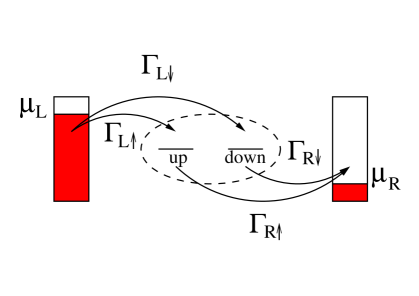
Figure 3.2: Schematic representation of the dynamics of the single dot device with spin. The two spin species can tunnel to and from the two degenerate spin levels of the quantum dot with rates $\Gamma_{L\uparrow},\Gamma_{L\downarrow}$ and $\Gamma_{R\uparrow},\Gamma_{R\downarrow}$, respectively and without influencing each other. Due to Coulomb blockade only one electron at a time can occupy the dot.

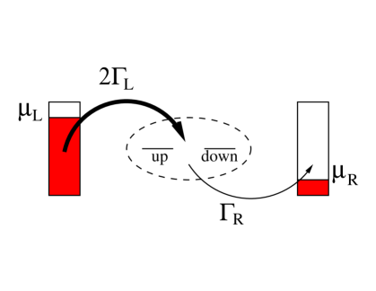
Figure 3.3: If we neglect the information of the spin specie the system dynamics can be reduced to the one of an effective spinless system with asymmetric injection and ejection rates.

which is an extension of the Hamiltonian (3.26) where $s=\pm 1/2$ is the spin degree of freedom and $U$ the charging energy of the double occupied dot. We take into account the interaction in the definition of the Hilbert space by discarding all the many-body states with double occupied dot. The effective Hamiltonian that we consider is then quadratic, and the Schrödinger equation projected onto the many-body basis gives rise to a recursive set of equations similar to (3.29). We have in this case three general equations corresponding to the three different states of the quantum dot:

$$\begin{split}i\dot{b}_{\{\uparrow l_{j}\}_{j=1}^{n_{\uparrow}}\{\downarrow l_{j}\}_{j=1}^{n_{\downarrow}}}&{}_{\{\uparrow r_{j}\}_{j=1}^{n_{\uparrow}}\{\downarrow r_{j}\}_{j=1}^{n_{\downarrow}}}=\\ &\left[\sum_{k=1}^{n_{\uparrow}+n_{\downarrow}}(\varepsilon_{r_{k}}-\varepsilon_{l_{k}})\right]b_{\{\uparrow l_{j}\}_{j=1}^{n_{\uparrow}}\{\downarrow l_{j}\}_{j=1}^{n_{\downarrow}}\{\uparrow r_{j}\}_{j=1}^{n_{\uparrow}}\{\downarrow r_{j}\}_{j=1}^{n_{\downarrow}}}\\ &+\sum_{l_{n_{\uparrow}+1}}\Omega_{l_{n_{\uparrow}+1}}b_{\uparrow\{\uparrow l_{j}\}_{j=1}^{n_{\uparrow}+1}\{\downarrow l_{j}\}_{j=1}^{n_{\downarrow}}\{\uparrow r_{j}\}_{j=1}^{n_{\uparrow}}\{\downarrow r_{j}\}_{j=1}^{n_{\downarrow}}}\\ &+\sum_{l_{n_{\downarrow}+1}}\Omega_{l_{n_{\downarrow}+1}}b_{\downarrow\{\uparrow l_{j}\}_{j=1}^{n_{\uparrow}}\{\downarrow l_{j}\}_{j=1}^{n_{\downarrow}+1}\{\uparrow r_{j}\}_{j=1}^{n_{\uparrow}}\{\downarrow r_{j}\}_{j=1}^{n_{\downarrow}}}\\ &+\sum_{k=1}^{n_{\uparrow}}(-1)^{k-n_{\uparrow}}\Omega_{r_{k}}b_{\uparrow\{\uparrow l_{j}\}_{j=1}^{n_{\uparrow}}\{\downarrow l_{j}\}_{j=1}^{n_{\downarrow}}\{\uparrow r_{j}\}_{j=1}^{n_{\uparrow}}\backslash\{\uparrow r_{k}\}\{\downarrow r_{j}\}_{j=1}^{n_{\downarrow}}}\\ &+\sum_{k=1}^{n_{\downarrow}}(-1)^{k-n_{\downarrow}}\Omega_{r_{k}}b_{\downarrow\{\uparrow l_{j}\}_{j=1}^{n_{\uparrow}}\{\downarrow l_{j}\}_{j=1}^{n_{\downarrow}}\{\uparrow r_{j}\}_{j=1}^{n_{\uparrow}}\{\downarrow r_{j}\}_{j=1}^{n_{\downarrow}}\backslash\{\downarrow r_{k}\}}\\ \end{split}$$ (3.61)

for the empty dot coefficient,

$$\begin{split}i\dot{b}_{\uparrow\{\uparrow l_{j}\}_{j=1}^{n_{\uparrow}+1}\{\downarrow l_{j}\}_{j=1}^{n_{\downarrow}}}&{}_{\{\uparrow r_{j}\}_{j=1}^{n_{\uparrow}}\{\downarrow r_{j}\}_{j=1}^{n_{\downarrow}}}=\\ &\left[\varepsilon_{1}+\sum_{k=1}^{n_{\uparrow}+n_{\downarrow}}(\varepsilon_{r_{k}}-\varepsilon_{l_{k}})-\varepsilon_{l_{n_{\uparrow}+1}}\right]b_{\{\uparrow l_{j}\}_{j=1}^{n_{\uparrow}+1}\{\downarrow l_{j}\}_{j=1}^{n_{\downarrow}}\{\uparrow r_{j}\}_{j=1}^{n_{\uparrow}}\{\downarrow r_{j}\}_{j=1}^{n_{\downarrow}}}\\ &+\sum_{r_{n_{\uparrow}+1}}\Omega_{r_{n_{\uparrow}+1}}b_{\{\uparrow l_{j}\}_{j=1}^{n_{\uparrow}+1}\{\downarrow l_{j}\}_{j=1}^{n_{\downarrow}}\{\uparrow r_{j}\}_{j=1}^{n_{\uparrow}+1}\{\downarrow r_{j}\}_{j=1}^{n_{\downarrow}}}\\ &+\sum_{k=1}^{n_{\uparrow}+1}(-1)^{k-n_{\uparrow}-1}\Omega_{l_{k}}b_{\{\uparrow l_{j}\}_{j=1}^{n_{\uparrow}+1}\backslash\{\uparrow l_{k}\}\{\downarrow l_{j}\}_{j=1}^{n_{\downarrow}}\{\uparrow r_{j}\}_{j=1}^{n_{\uparrow}}\{\downarrow r_{j}\}_{j=1}^{n_{\downarrow}}}\\ \end{split}$$ (3.62)

for the spin-up and finally

$$\begin{split}i\dot{b}_{\downarrow\{\uparrow l_{j}\}_{j=1}^{n_{\uparrow}}\{\downarrow l_{j}\}_{j=1}^{n_{\downarrow}+1}}&{}_{\{\uparrow r_{j}\}_{j=1}^{n_{\uparrow}}\{\downarrow r_{j}\}_{j=1}^{n_{\downarrow}}}=\\ &\left[\varepsilon_{1}+\sum_{k=1}^{n_{\uparrow}+n_{\downarrow}}(\varepsilon_{r_{k}}-\varepsilon_{l_{k}})-\varepsilon_{l_{n_{\downarrow}+1}}\right]b_{\{\uparrow l_{j}\}_{j=1}^{n_{\uparrow}}\{\downarrow l_{j}\}_{j=1}^{n_{\downarrow}+1}\{\uparrow r_{j}\}_{j=1}^{n_{\uparrow}}\{\downarrow r_{j}\}_{j=1}^{n_{\downarrow}}}\\ &+\sum_{r_{n_{\uparrow}+1}}\Omega_{r_{n_{\downarrow}+1}}b_{\{\uparrow l_{j}\}_{j=1}^{n_{\uparrow}+1}\{\downarrow l_{j}\}_{j=1}^{n_{\downarrow}}\{\uparrow r_{j}\}_{j=1}^{n_{\uparrow}}\{\downarrow r_{j}\}_{j=1}^{n_{\downarrow}+1}}\\ &+\sum_{k=1}^{n_{\downarrow}+1}(-1)^{k-n_{\downarrow}-1}\Omega_{l_{k}}b_{\{\uparrow l_{j}\}_{j=1}^{n_{\uparrow}}\{\downarrow l_{j}\}_{j=1}^{n_{\downarrow}+1}\backslash\{\downarrow l_{k}\}\{\uparrow r_{j}\}_{j=1}^{n_{\uparrow}}\{\downarrow r_{j}\}_{j=1}^{n_{\downarrow}}}\end{split}$$ (3.63)

for the spin-down coefficient. In the last three differential equations (3.61), (3.62) and (3.63) we have extended the notation used in equation (3.29) to take into account the spin degree of freedom. Despite the heavy but complete notation that keeps track of the four baths (two leads with two spin species per lead) and the state of the dot, the same kind of arguments that we used for the spin-less case bring us to the set of rate equations:

$$\begin{split}\dot{\sigma}_{00}^{(n)}&=-(\Gamma_{L\uparrow}+\Gamma_{L\downarrow})\sigma_{00}^{(n)}+\Gamma_{R\uparrow}\sigma_{\uparrow\uparrow}^{(n-1)}+\Gamma_{R\downarrow}\sigma_{\downarrow\downarrow}^{(n-1)}\\ \dot{\sigma}_{\uparrow\uparrow}^{(n)}&=-\Gamma_{R\uparrow}\sigma_{\uparrow\uparrow}^{(n)}+\Gamma_{L\uparrow}\sigma_{00}^{(n)}\\ \dot{\sigma}_{\downarrow\downarrow}^{(n)}&=-\Gamma_{R\downarrow}\sigma_{\downarrow\downarrow}^{(n)}+\Gamma_{L\downarrow}\sigma_{00}^{(n)}\end{split}$$ (3.64)

where $\sigma_{\uparrow\uparrow}^{(n)}$ ($\sigma_{\downarrow\downarrow}^{(n)}$) is the population of spin up (down) in the dot with $n=n_{\uparrow}+n_{\downarrow}$ electrons in the collector and we have introduced the spin-dependent injection and ejection rates:

$$\begin{split}\Gamma_{L,R\uparrow}&=2\pi D_{L,R\uparrow}\Omega_{L,R}^{2}\\ \Gamma_{L,R\downarrow}&=2\pi D_{L,R\downarrow}\Omega_{L,R}^{2}\end{split}$$ (3.65)

The sum over the number of electrons in the collector gives:

$$\begin{split}\dot{\sigma}_{00}&=-(\Gamma_{L\uparrow}+\Gamma_{L\downarrow})\sigma_{00}+\Gamma_{R\uparrow}\sigma_{\uparrow\uparrow}+\Gamma_{R\downarrow}\sigma_{\downarrow\downarrow}\\ \dot{\sigma}_{\uparrow\uparrow}&=-\Gamma_{R\uparrow}\sigma_{\uparrow\uparrow}+\Gamma_{L\uparrow}\sigma_{00}\\ \dot{\sigma}_{\downarrow\downarrow}&=-\Gamma_{R\downarrow}\sigma_{\downarrow\downarrow}+\Gamma_{L\downarrow}\sigma_{00}\\ \end{split}$$ (3.66)

The coherencies between different spin species in the QD (e.g. $\sigma_{\uparrow\downarrow}$) vanish in this model because different spin states of the dot correspond to different bath states and the only way to have coherent superpositions in the dot would be to maintain the same in the leads which instead are assumed (as macroscopic objects) incoherent. If we are not interested in the spin information on the dot we can introduce the population for the charged dot $\sigma_{11}^{(n)}\equiv\sigma_{\uparrow\uparrow}^{(n)}+\sigma_{\downarrow\downarrow}^{(n)}$. Assuming also non-polarized leads (i.e. $D_{L,R\uparrow}=D_{L,R\downarrow}$) and, consequently, tunneling rates independent of different spin species the system of rate equations (3.66) becomes:

$$\begin{split}\dot{\sigma}_{00}&=-2\Gamma_{L}\sigma_{00}+\Gamma_{R}\sigma_{11}\\ \dot{\sigma}_{11}&=-\Gamma_{R}\sigma_{11}+2\Gamma_{L}\sigma_{00}\end{split}$$ (3.67)

where $\Gamma_{L}=\Gamma_{L\uparrow}=\Gamma_{L\downarrow}$ and $\Gamma_{R}=\Gamma_{R\uparrow}=\Gamma_{R\downarrow}$. Comparing these rate equations with the ones derived for the spin-less non-interacting model (3.57) we note that the only remaining signature of the spin degree of freedom is in the injection rate. In the case of identical leads the injection rate doubles the ejection rate. This behaviour can be interpreted in terms of tunneling channels: both spin species can tunnel in when the dot is empty, but once the dot is charged with an electron of specific spin only that species can tunnel out. At this level the spin degree of freedom is just renormalizing the injection rate. Since this argument can be repeated for any model in strong Coulomb blockade we will restrict the derivation of the GME for shuttling devices to spin-less non-interacting particles.

3.3.7 Coherencies and double-dot model

A simple example of a device that exhibits coherent transport is represented by an array of two quantum dots located between a source and a drain lead. We assume that the device is working in strong Coulomb blockade (i.e. only one electron at a time can occupy the device, either in the left or in the right dot). Electrons can tunnel in the device from the emitter only to the left dot while tunneling off is allowed only from the right dot. This condition can be achieved due to the fact that the tunneling coupling to the leads decreases exponentially with the distance and can be neglected for the far lead. Also the two dots are in tunneling contact. Since the transport must happen via tunneling between the discrete levels of the dots we expect coherencies to play a role. The Hamiltonian for the model reads:

$$\begin{split}H=&\varepsilon_{L}|L\rangle\!\langle L|+\Omega_{0}(|L\rangle\!\langle R|+|R\rangle\!\langle L|)+\varepsilon_{R}|R\rangle\!\langle R|\\ &+\sum_{l}\varepsilon_{l}c_{l}^{\dagger}c_{l}^{\phantom{\dagger}}+\sum_{r}\varepsilon_{r}c_{r}^{\dagger}c_{r}^{\phantom{\dagger}}\\ &+\sum_{l}\Omega_{l}(|L\rangle\!\langle 0|c_{l}^{\phantom{\dagger}}+|0\rangle\!\langle L|c_{l}^{{\dagger}})+\sum_{r}\Omega_{r}(|R\rangle\!\langle 0|c_{r}^{\phantom{\dagger}}+|0\rangle\!\langle R|c_{r}^{{\dagger}})\end{split}$$ (3.68)

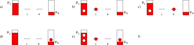
Figure 3.4: Schematic representation of the first many-body basis elements for the double dot system.

We identify in the first line the system Hamiltonian with the single energy levels of the left and right dot ($\varepsilon_{L}$ and $\varepsilon_{R}$) and the tunneling amplitude $\Omega_{0}$. The second and third lines describe respectively the electronic baths (the leads) and their coupling to the device. The system can be found, as in the spin model, in three different states: empty or occupied with an electron either in the left or right dot. We associate to each of these states the vectors $|0\rangle$, $|L\rangle$ and $|R\rangle$. The Schrödinger equation projected onto the many-body basis for the system+baths Hilbert space can be then represented by the following three recursive differential equations for the expansion coefficients:

$$\begin{split}i\dot{b}_{\{l_{j}\}_{j=1}^{n}\{r_{j}\}_{j=1}^{n}}=&\left[\sum_{k=1}^{n}(\varepsilon_{r_{k}}-\varepsilon_{l_{k}})\right]b_{\{l_{j}\}_{j=1}^{n}\{r_{j}\}_{j=1}^{n}}\\ &\!\!\!+\sum_{l_{n+1}}\Omega_{l_{n+1}}b_{L\{l_{j}\}_{j=1}^{n+1}\{r_{j}\}_{j=1}^{n}}\!\!+\sum_{k=1}^{n}(-1)^{k-n}\Omega_{r_{k}}b_{R\{l_{j}\}_{j=1}^{n}\{r_{j}\}_{j=1}^{n}\backslash\{r_{k}\}}\\ i\dot{b}_{L\{l_{j}\}_{j=1}^{n+1}\{r_{j}\}_{j=1}^{n}}=&\left[\varepsilon_{L}+\sum_{k=1}^{n}(\varepsilon_{r_{k}}-\varepsilon_{l_{k}})-\varepsilon_{l_{n+1}}\right]b_{L\{l_{j}\}_{j=1}^{n+1}\{r_{j}\}_{j=1}^{n}}\\ &\!\!\!+\Omega_{0}b_{R\{l_{j}\}_{j=1}^{n+1}\{r_{j}\}_{j=1}^{n}}+\sum_{k=1}^{n+1}(-1)^{k-n-1}\Omega_{l_{k}}b_{\{l_{j}\}_{j=1}^{n+1}\backslash\{l_{k}\}\{r_{j}\}_{j=1}^{n}}\\ i\dot{b}_{R\{l_{j}\}_{j=1}^{n+1}\{r_{j}\}_{j=1}^{n}}=&\left[\varepsilon_{R}+\sum_{k=1}^{n}(\varepsilon_{r_{k}}-\varepsilon_{l_{k}})-\varepsilon_{l_{n+1}}\right]b_{R\{l_{j}\}_{j=1}^{n+1}\{r_{j}\}_{j=1}^{n}}\\ &\!\!\!+\Omega_{0}b_{L\{l_{j}\}_{j=1}^{n+1}\{r_{j}\}_{j=1}^{n}}+\sum_{r_{n+1}}\Omega_{r_{n+1}}b_{\{l_{j}\}_{j=1}^{n+1}\{r_{j}\}_{j=1}^{n+1}}\end{split}$$ (3.69)

The Laplace transform can be taken and the continuous sums in the first and third equation be performed to give the set of algebraic equations:

$$\begin{split}&\left[E+\sum_{k=1}^{n}(\varepsilon_{r_{k}}-\varepsilon_{l_{k}})+i\frac{\Gamma_{L}}{2}\right]\tilde{b}_{\{l_{j}\}_{j=1}^{n}\{r_{j}\}_{j=1}^{n}}(E)\\ &\phantom{aaaaa}-\sum_{k=1}^{n}(-1)^{k-n}\Omega_{r_{k}}\tilde{b}_{R\{l_{j}\}_{j=1}^{n}\{r_{j}\}_{j=1}^{n}\backslash\{r_{k}\}}(E)=i\delta_{n0}\\ &\left[E+\varepsilon_{L}+\sum_{k=1}^{n}(\varepsilon_{r_{k}}-\varepsilon_{l_{k}})-\varepsilon_{l_{n+1}}\right]\tilde{b}_{L\{l_{j}\}_{j=1}^{n+1}\{r_{j}\}_{j=1}^{n}}(E)\\ &\phantom{aaaaa}-\Omega_{0}\tilde{b}_{R\{l_{j}\}_{j=1}^{n+1}\{r_{j}\}_{j=1}^{n}}(E)-\sum_{k=1}^{n+1}(-1)^{k-n-1}\Omega_{l_{k}}\tilde{b}_{\{l_{j}\}_{j=1}^{n+1}\backslash\{l_{k}\}\{r_{j}\}_{j=1}^{n}}(E)=0\\ &\left[E+\varepsilon_{R}+\sum_{k=1}^{n}(\varepsilon_{r_{k}}-\varepsilon_{l_{k}})-\varepsilon_{l_{n+1}}+i\frac{\Gamma_{R}}{2}\right]\tilde{b}_{R\{l_{j}\}_{j=1}^{n+1}\{r_{j}\}_{j=1}^{n}}(E)\\ &\phantom{aaaaa}-\Omega_{0}\tilde{b}_{L\{l_{j}\}_{j=1}^{n+1}\{r_{j}\}_{j=1}^{n}}(E)=0\end{split}$$ (3.70)

In the double dot model some coherencies of the reduced density matrix do not vanish since they correspond to different “internal” states of the dot and can be combined with the same state of the baths. For example:

$$\begin{split}\sigma_{LR}^{(n)}(t)&=\sum_{\{B_{n}\}}\langle L,B_{n}|\Psi(t)\rangle\!\langle\Psi(t)|R,B_{n}\rangle\\ &=\sum_{\{l_{k}\}\{r_{k}\}}b_{L\{l_{k}\}_{k=1}^{n+1}\{r_{k}\}_{k=1}^{n}}(t)b_{R\{l_{k}\}_{k=1}^{n+1}\{r_{k}\}_{k=1}^{n}}^{*}(t)\end{split}$$ (3.71)

The next step is an $n$-resolved GME for the reduced density matrix $\sigma$. The equations for the populations are derived following the procedure we explained for the single dot model:

$$\begin{split}\dot{\sigma}_{00}^{(n)}&=-\Gamma_{L}\sigma_{00}^{(n)}+\Gamma_{R}\sigma_{RR}^{(n-1)}\\ \dot{\sigma}_{LL}^{(n)}&=-i\Omega_{0}\left(\sigma_{RL}^{(n)}-\sigma_{LR}^{(n)}\right)+\Gamma_{L}\sigma_{00}^{n}\\ \dot{\sigma}_{RR}^{(n)}&=-\Gamma_{R}\sigma_{RR}^{(n)}-i\Omega_{0}\left(\sigma_{LR}^{(n)}-\sigma_{RL}^{(n)}\right)\end{split}$$ (3.72)

The coherencies play an active role in the transport through the quantum dots: the second and third equations in (3.72) show that the left (right) dot can be discharged (charged) only via coherent transport. We concentrate now on the equation for the coherence $\sigma_{LR}^{(n)}$. We take the second equation in (3.70) and multiply it by $\tilde{b}_{R\{l_{j}\}_{j=1}^{n+1}\{r_{j}\}_{j=1}^{n}}^{*}(E^{\prime})e^{-i(E-E^{\prime})t}$, then we subtract side by side the complex conjugate of the third equation in (3.70) evaluated in $E^{\prime}$ and multiplied by $\tilde{b}_{L\{l_{j}\}_{j=1}^{n+1}\{r_{j}\}_{j=1}^{n}}(E)e^{-i(E-E^{\prime})t}$. Finally we integrate over $dE$ and $dE^{\prime}$ and sum over the baths configurations with $n$ electrons in the collector. Using the properties of the Laplace transform and the representation of the reduced density matrix in terms of the coefficients $b$ of the many-body expansion we obtain:

$$\begin{split}&i\dot{\sigma}_{LR}^{(n)}(t)+\Big{(}\varepsilon_{L}-\varepsilon_{R}+i\frac{\Gamma_{R}}{2}\Big{)}\sigma_{LR}^{(n)}(t)-\Omega_{0}\Big{[}\sigma_{RR}^{(n)}(t)-\sigma_{LL}^{(n)}(t)\Big{]}\\ &-\sum_{\{l_{j}\}\{r_{j}\}}\int\frac{dEdE^{\prime}}{4\pi^{2}}\Big{[}\sum_{k=1}^{n+1}(-1)^{k-n-1}\Omega_{l_{k}}\tilde{b}_{\{l_{j}\}_{j=1}^{n+1}\backslash\{l_{k}\}\{r_{j}\}_{j=1}^{n}}(E)\\ &\tilde{b}_{R\{l_{j}\}_{j=1}^{n+1}\{r_{j}\}_{j=1}^{n}}^{*}(E^{\prime})e^{-i(E-E^{\prime})t}\Big{]}=0\end{split}$$ (3.73)

The last term in the LHS of equation (3.73) vanishes since the integrand behaves asymptotically as $o(|\varepsilon_{l_{j},r_{j}}|^{-1})$ in the limit $|\varepsilon_{l_{j},r_{j}}|\to\infty$ for all the integrated variables $\varepsilon_{l_{j},r_{j}}$. The average over the bath degrees of freedom is completed by the sum over the number of electrons in the collector $n$ that leads to the GME:

$$\begin{split}\dot{\sigma}_{00}&=-\Gamma_{L}\sigma_{00}+\Gamma_{R}\sigma_{RR}\\ \dot{\sigma}_{LL}&=-i\Omega_{0}(\sigma_{RL}-\sigma_{LR})+\Gamma_{L}\sigma_{00}\\ \dot{\sigma}_{RR}&=-\Gamma_{R}\sigma_{RR}-i\Omega_{0}(\sigma_{LR}-\sigma_{RL})\\ \dot{\sigma}_{LR}&=-i(\varepsilon_{L}-\varepsilon_{R})\sigma_{LR}-\textstyle{\frac{1}{2}}\Gamma_{R}\sigma_{LR}-i\Omega_{0}(\sigma_{RR}-\sigma_{LL})\end{split}$$ (3.74)

where we have omitted the equation for ${\sigma}_{RL}$ since $\sigma$ is a hermitian operator on the Hilbert space of the system and $\sigma_{RL}=\sigma_{LR}^{*}$. We can better visualize the coherent and incoherent contribution to the GME using a matrix representation:

$$\dot{\sigma}=-i[H_{sys},\sigma]+\Xi[\sigma]$$ (3.75)

where $\sigma$ is the density matrix

$$\sigma=\left(\begin{array}[]{ccc}\sigma_{00}&\sigma_{0L}&\sigma_{0R}\\ \sigma_{L0}&\sigma_{LL}&\sigma_{LR}\\ \sigma_{R0}&\sigma_{RL}&\sigma_{RR}\\ \end{array}\right),$$ (3.76)

$H_{sys}$ is the Hamiltonian for the system extended to the empty state for the system

$$H_{sys}=\left(\begin{array}[]{ccc}0&0&0\\ 0&\varepsilon_{L}&\Omega_{0}\\ 0&\Omega_{0}&\varepsilon_{R}\\ \end{array}\right)$$ (3.77)

and $\Xi[\bullet]$ is a linear super-operator that transform operators on the Hilbert space of the system into operators on the same space and acts on the density matrix:

$$\Xi[\sigma]=\left(\begin{array}[]{ccc}-\Gamma_{L}\sigma_{00}+\Gamma_{R}\sigma_{RR}&0&0\\ 0&\Gamma_{L}\sigma_{00}&-\frac{1}{2}\Gamma_{R}\sigma_{LR}\\ 0&-\frac{1}{2}\Gamma_{R}\sigma_{RL}&-\Gamma_{R}\sigma_{RR}\\ \end{array}\right)$$ (3.78)

3.4 GME for shuttle devices

The shuttle devices are in contact with two different kinds of bath: two electrical baths (the leads) and a mechanical bath. We assume that the electrical and mechanical baths act independently on the device. This assumption splits the GME into two additive components, one for each kind of bath. Due to the different coupling strengths we derive the electrical component extending the method proposed by Gurvitz and extensively presented in Section 3.3 while for the mechanical component we adopt the weak coupling quantum optical derivation presented in Section 3.2.

3.4.1 Single Dot Quantum Shuttle

We start recalling the Hamiltonian for the SDQS:

$$H=H_{\rm sys}+H_{\rm leads}+H_{\rm bath}+H_{\rm tun}+H_{\rm int}$$ (3.79)

where

$$\begin{split}&H_{\rm sys}=\frac{\hat{p}^{2}}{2m}+\frac{1}{2}m\omega^{2}\hat{x}^{2}+(\varepsilon_{1}-e\mathcal{E}\hat{x})c_{1}^{{\dagger}}c_{1}^{\phantom{\dagger}}\\ &H_{\rm leads}=\sum_{k}(\varepsilon_{l_{k}}c^{\dagger}_{l_{k}}c^{\phantom{\dagger}}_{l_{k}}+\varepsilon_{r_{k}}c^{\dagger}_{r_{k}}c^{\phantom{\dagger}}_{r_{k}})\\ &H_{\rm tun}=\sum_{k}[T_{l}(\hat{x})c^{\dagger}_{l_{k}}c_{1}^{\phantom{\dagger}}+T_{r}(\hat{x})c^{\dagger}_{r_{k}}c_{1}^{\phantom{\dagger}}]+h.c.\\ &H_{\rm bath}+H_{\rm int}={\rm generic\;heat\;bath}\end{split}$$ (3.80)

Also the mechanical degree of freedom is treated quantum mechanically. For example the position operator can be expressed in the form:

$$\hat{x}=\sqrt{\frac{\hbar}{2m\omega}}(d^{{\dagger}}+d)$$ (3.81)

where $d^{{\dagger}}$ and $d$ are respectively the creation and annihilation operators for the harmonic oscillator. We neglect for a moment the mechanical bath and its coupling to the system and start the Gurvitz analysis of the model dynamics. The many-body basis introduced in (3.27) must be extended to take into account also the phononic excitations of the system. For definiteness we choose the eigenvectors of the oscillator Hamiltonian as a basis for the mechanical part. We display the basis elements in the following table:

r=0 r=1 r=2 $$\ldots$$

(3.82)

where $r$ is the number of excitations of the oscillator and the empty state $|0\rangle$ represents the empty dot in its mechanical ground state with leads filled up to their Fermi energies. It is convenient to organize the coefficients of the expansion of the state vector $|\Psi\rangle$ in the basis (3.82) in vectors: one for each electronic configuration. The different elements of the vectors refer to the different excited states for the oscillator. The Schrödinger equation for the state vector $|\Psi\rangle$ is represented in the basis (3.82) by two recursive differential equations for the vector coefficients $\mathbf{b}$’s:

$$\begin{split}i\dot{\mathbf{b}}_{\{l_{j}\}_{j=1}^{n}}&{}_{\{r_{j}\}_{j=1}^{n}}=\left[\hat{H}_{\rm osc}+\sum_{k=1}^{n}(\varepsilon_{r_{k}}-\varepsilon_{l_{k}})\right]\mathbf{b}_{\{l_{j}\}_{j=1}^{n}\{r_{j}\}_{j=1}^{n}}\\ &+\sum_{l_{n+1}}T_{l}(\hat{x})\mathbf{b}_{1\{l_{j}\}_{j=1}^{n+1}\{r_{j}\}_{j=1}^{n}}+\sum_{k=1}^{n}(-1)^{k-n}T_{r}(\hat{x})\mathbf{b}_{1\{l_{j}\}_{j=1}^{n}\{r_{j}\}_{j=1}^{n}\backslash\{r_{k}\}}\\ i\dot{\mathbf{b}}_{1\{l_{j}\}_{j=1}^{n+1}}&{}_{\{r_{j}\}_{j=1}^{n}}=\left[\hat{H}_{\rm osc}+\varepsilon_{1}-e\mathcal{E}\hat{x}+\sum_{k=1}^{n}(\varepsilon_{r_{k}}-\varepsilon_{l_{k}})-\varepsilon_{l_{n+1}}\right]\mathbf{b}_{1\{l_{j}\}_{j=1}^{n+1}\{r_{j}\}_{j=1}^{n}}\\ &+\sum_{r_{n+1}}T_{r}(\hat{x})\mathbf{b}_{\{l_{j}\}_{j=1}^{n+1}\{r_{j}\}_{j=1}^{n+1}}+\sum_{k=1}^{n+1}(-1)^{k-n-1}T_{l}(\hat{x})\mathbf{b}_{\{l_{j}\}_{j=1}^{n+1}\backslash\{l_{k}\}\{r_{j}\}_{j=1}^{n}}\\ \end{split}$$ (3.83)

where $\hat{x}$ is given in its matrix representation in terms of the occupation number basis ($\hbar=1$):

$$\hat{x}_{rs}=\sqrt{\frac{r}{2m\omega}}(\delta_{r,s+1}+\delta_{r,s-1})$$ (3.84)

and the Hamiltonian for the harmonic oscillator in the same basis reads:

$$\hat{H}_{\rm osc}=\omega\left(\frac{1}{2}+r\delta_{rs}\right)$$ (3.85)

All the constants in equation (3.83) are identity operators in the mechanical Hilbert space.

One of the key assumptions in the derivation of the GME in the Gurvitz approach is the position of the energy levels of the system: they must lie well inside the transport window open between the chemical potentials of the leads. Since the oscillator spectrum is not bounded from above we assume that only a finite number of mechanical excitations are involved in the dynamics of the system. We will see that, at least in the presence of a mechanical bath, this assumption is numerically fulfilled. In any case a violation of this condition in the final result would be unacceptable since it would violate the validity condition of the GME. From the point of view of the experimental realization of the device this limit is imposed at least by the leads that set an upper bound to the amplitude of the dot oscillations.

The Laplace transform of (3.83) with the initial condition $|\Psi(t=0)\rangle=|0\rangle$ reads:

$$\begin{split}&\left[E+\hat{H}_{\rm osc}+\sum_{k=1}^{n}(\varepsilon_{r_{k}}-\varepsilon_{l_{k}})\right]\tilde{\mathbf{b}}_{\{l_{j}\}_{j=1}^{n}\{r_{j}\}_{j=1}^{n}}(E)-\sum_{l_{n+1}}T_{l}(\hat{x})\tilde{\mathbf{b}}_{1\{l_{j}\}_{j=1}^{n+1}\{r_{j}\}_{j=1}^{n}}(E)\\ &\phantom{a}-\sum_{k=1}^{n}(-1)^{k-n}T_{r}(\hat{x})\tilde{\mathbf{b}}_{1\{l_{j}\}_{j=1}^{n}\{r_{j}\}_{j=1}^{n}\backslash\{r_{k}\}}(E)=i\delta_{n0}\mathbf{v}_{0}\\ &\left[E+\hat{H}_{\rm osc}+\varepsilon_{1}-e\mathcal{E}\hat{x}+\sum_{k=1}^{n}(\varepsilon_{r_{k}}-\varepsilon_{l_{k}})-\varepsilon_{l_{n+1}}\right]\tilde{\mathbf{b}}_{1\{l_{j}\}_{j=1}^{n+1}\{r_{j}\}_{j=1}^{n}}(E)\\ &\phantom{a}-\!\sum_{r_{n+1}}T_{r}(\hat{x})\tilde{\mathbf{b}}_{\{l_{j}\}_{j=1}^{n+1}\{r_{j}\}_{j=1}^{n+1}}(E)-\!\sum_{k=1}^{n+1}(-1)^{k-n-1}T_{l}(\hat{x})\tilde{\mathbf{b}}_{\{l_{j}\}_{j=1}^{n+1}\backslash\{l_{k}\}\{r_{j}\}_{j=1}^{n}}(E)=0\end{split}$$ (3.86)

where $\mathbf{v}_{0}$ is the initial condition of the oscillator.

The continuous sums in the system (3.86) can be performed with an argument similar to the one used for the static QD. We have just to be careful with the matrix notation and change the basis to diagonalize the matrix:

$$M=\left[E+\hat{H}_{\rm osc}+\varepsilon_{1}-e\mathcal{E}\hat{x}+\sum_{k=1}^{n}(\varepsilon_{r_{k}}-\varepsilon_{l_{k}})-\varepsilon_{l_{n+1}}\right]$$ (3.87)

before taking the integral. The sum $\sum_{r_{n+1}}$ in the second Eq. of (3.86) can be treated analogously. As in the static case the continuous sums are condensed into “rates”:

$$\begin{split}&\left[E+\hat{H}_{\rm osc}+\sum_{k=1}^{n}(\varepsilon_{r_{k}}-\varepsilon_{l_{k}})-i\frac{\Gamma_{L}(\hat{x})}{2}\right]\tilde{\mathbf{b}}_{\{l_{j}\}_{j=1}^{n}\{r_{j}\}_{j=1}^{n}}(E)\\ &\phantom{aaaaaa}-\sum_{k=1}^{n}(-1)^{k-n}T_{r}(\hat{x})\tilde{\mathbf{b}}_{1\{l_{j}\}_{j=1}^{n}\{r_{j}\}_{j=1}^{n}\backslash\{r_{k}\}}(E)=i\delta_{n0}\mathbf{v}_{0}\\ &\left[E+\hat{H}_{\rm osc}+\varepsilon_{1}-e\mathcal{E}\hat{x}+\sum_{k=1}^{n}(\varepsilon_{r_{k}}-\varepsilon_{l_{k}})-\varepsilon_{l_{n+1}}-i\frac{\Gamma_{R}(\hat{x})}{2}\right]\tilde{\mathbf{b}}_{1\{l_{j}\}_{j=1}^{n+1}\{r_{j}\}_{j=1}^{n}}(E)\\ &\phantom{aaaaaa}-\sum_{k=1}^{n+1}(-1)^{k-n-1}T_{l}(\hat{x})\tilde{\mathbf{b}}_{\{l_{j}\}_{j=1}^{n+1}\backslash\{l_{k}\}\{r_{j}\}_{j=1}^{n}}(E)=0\end{split}$$ (3.88)

where

$$\Gamma_{L,R}(\hat{x})=2\pi D_{L,R}T^{2}_{l,r}(\hat{x})=\Gamma_{L,R}\,e^{\mp 2\hat{x}/\lambda}$$ (3.89)

and we have introduced the tunneling length $\lambda$ and the bare injection (ejection) rate $\Gamma_{L}$ ($\Gamma_{R}$).

The reduced density matrix for the system contains information about the electrical occupation of the QD and its mechanical state. Coherencies between occupied and empty state vanish because they imply coherencies between states with different particle number in the baths. The equation (3.40) for the non-vanishing elements written in the static QD case still holds:

$$\sigma_{ii}(t)=\sum_{n=0}^{\infty}\sum_{\{B_{n}\}}\langle i_{S},B_{n}|\Psi(t)\rangle\!\langle\Psi(t)|B_{n},i_{S}\rangle=\sum_{n=0}^{\infty}\sigma_{ii}^{(n)}(t)$$ (3.90)

with the difference that the “elements” $\sigma_{ii}$ are now full operators in the mechanical Hilbert space. It is useful to express them in terms of the vectors $\mathbf{b}$:

$$\begin{split}\sigma_{00}^{(n)}(t)&=\sum_{\{l_{k}\}\{r_{k}\}}\mathbf{b}_{\{l_{k}\}_{k=1}^{n}\{r_{k}\}_{k=1}^{n}}(t)\mathbf{b}_{\{l_{k}\}_{k=1}^{n}\{r_{k}\}_{k=1}^{n}}^{{\dagger}}(t)\\ \sigma_{11}^{(n)}(t)&=\sum_{\{l_{k}\}\{r_{k}\}}\mathbf{b}_{1\{l_{k}\}_{k=1}^{n+1}\{r_{k}\}_{k=1}^{n}}(t)\mathbf{b}_{1\{l_{k}\}_{k=1}^{n+1}\{r_{k}\}_{k=1}^{n}}^{{\dagger}}(t)\end{split}$$ (3.91)

The notation of equation (3.91) can be understood in terms of the Dirac notation: $\mathbf{b}^{{\dagger}}$ is the bra of the corresponding vector $\mathbf{b}$ (the ket). The inverse Laplace transform brings us back to the vectors $\tilde{\mathbf{b}}$:

$$\begin{split}\sigma_{00}^{(n)}(t)&=\int\frac{dEdE^{\prime}}{4\pi^{2}}\sum_{\{l_{k}\}\{r_{k}\}}\tilde{\mathbf{b}}_{\{l_{k}\}_{k=1}^{n}\{r_{k}\}_{k=1}^{n}}(E)\tilde{\mathbf{b}}_{\{l_{k}\}_{k=1}^{n}\{r_{k}\}_{k=1}^{n}}^{{\dagger}}(E^{\prime})e^{-i(E-E^{\prime})t}\\ \sigma_{11}^{(n)}(t)&=\int\frac{dEdE^{\prime}}{4\pi^{2}}\sum_{\{l_{k}\}\{r_{k}\}}\tilde{\mathbf{b}}_{1\{l_{k}\}_{k=1}^{n+1}\{r_{k}\}_{k=1}^{n}}(E)\tilde{\mathbf{b}}_{1\{l_{k}\}_{k=1}^{n+1}\{r_{k}\}_{k=1}^{n}}^{{\dagger}}(E^{\prime})e^{-i(E-E^{\prime})t}\end{split}$$ (3.92)

The case with $n=0$ must be treated separately. The inverse Laplace transform of the first equation in the system (3.88) specialized for $n=0$ reads:

$$i\dot{\mathbf{b}}_{0}=\hat{H}_{\rm osc}\mathbf{b}_{0}-i\frac{\Gamma_{L}(\hat{x})}{2}\mathbf{b}_{0}$$ (3.93)

and its Hermitian conjugate:

$$-i\dot{\mathbf{b}}_{0}^{{\dagger}}=\mathbf{b}_{0}^{{\dagger}}\hat{H}_{\rm osc}+i\mathbf{b}_{0}^{{\dagger}}\frac{\Gamma_{L}(\hat{x})}{2}$$ (3.94)

where we have used the property of adjoint of vectors and operators $(AB)^{{\dagger}}=B^{{\dagger}}A^{{\dagger}}$ and the fact that the oscillator Hamiltonian and position operator are Hermitian on the mechanical Hilbert space. The combination of equations (3.91), (3.93), (3.94) and the Leibnitz rule for derivatives extended to the tensor product between vectors and linear forms lead to the first component of the GME for the SDQS:

$$\dot{\sigma}_{00}^{(0)}(t)=-i\Big{[}\hat{H}_{\rm osc},\sigma_{00}^{(0)}\Big{]}-\frac{\Gamma_{L}}{2}\Big{\{}e^{-2\hat{x}/\lambda},\sigma_{00}^{(0)}\Big{\}}$$ (3.95)

where $[A,B]\equiv AB-BA$ is the commutator and $\{A,B\}\equiv AB+BA$ the anticommutator between the operators $A$ and $B$. Equation (3.95) already contains the essence of the driving part of the GME: a coherent evolution represented by the commutator with the oscillator Hamiltonian and a non-coherent term due to the interaction with the bath. In this second contribution the quantum features are given by the particular ordering of the operators.

For the general case with $n\neq 0$ the procedure is to take the first equation of (3.88) evaluated in $E$ and make the tensor product with $\tilde{\mathbf{b}}_{\{l_{j}\}_{j=1}^{n}\{r_{j}\}_{j=1}^{n}}^{{\dagger}}(E^{\prime})$ $e^{-i(E-E^{\prime})t}$, subtract side by side the adjoint of the first equation in (3.88) evaluated in $E^{\prime}$ multiplied (from the right) with the vector $\tilde{\mathbf{b}}_{\{l_{j}\}_{j=1}^{n}\{r_{j}\}_{j=1}^{n}}(E)$ $e^{-i(E-E^{\prime})t}$, integrate in $dE$ and $dE^{\prime}$ and sum over the possible bath configuration with $n$ extra electrons in the right lead. Using the properties of the Laplace transform and the representation of the reduced density matrix in terms of the vectors $\mathbf{b}$ (3.91) we get:

$$\begin{split}i\dot{\sigma}&{}_{00}^{(n)}-\Big{[}\hat{H}_{\rm osc},\sigma_{00}^{(n)}\Big{]}-i\frac{\Gamma_{L}}{2}\Big{\{}e^{-2\hat{x}/\lambda},\sigma_{00}^{(n)}\Big{\}}\\ &-\!\!\sum_{\{l_{j}\}\{r_{j}\}}\!\!\int\frac{dEdE^{\prime}}{4\pi^{2}}\!\sum_{k=1}^{n}(-1)^{k-n}\Big{[}T_{r}(\hat{x})\tilde{\mathbf{b}}_{1\{l_{j}\}_{j=1}^{n}\{r_{j}\}_{j=1}^{n}\backslash\{r_{k}\}}(E)\tilde{\mathbf{b}}_{\{l_{j}\}_{j=1}^{n}\{r_{j}\}_{j=1}^{n}}^{{\dagger}}(E^{\prime})\\ &-\tilde{\mathbf{b}}_{\{l_{j}\}_{j=1}^{n}\{r_{j}\}_{j=1}^{n}}(E)\tilde{\mathbf{b}}_{1\{l_{j}\}_{j=1}^{n}\{r_{j}\}_{j=1}^{n}\backslash\{r_{k}\}}^{{\dagger}}(E^{\prime})T_{r}(\hat{x})\Big{]}e^{-i(E-E^{\prime})t}=0\end{split}$$ (3.96)

We solve the first equation in (3.88) with respect to $\tilde{\mathbf{b}}_{\{l_{j}\}_{j=1}^{n}\{r_{j}\}_{j=1}^{n}}$. Then we insert the result and its adjoint in (3.96) and, as in the static QD, we are left with the only non-vanishing continuous sum in the “missing” variable $r_{n}$. The result is the matrix equation:

$$\dot{\sigma}_{00}^{(n)}=-i\Big{[}\hat{H}_{\rm osc},\sigma_{00}^{(n)}\Big{]}-\frac{\Gamma_{L}}{2}\Big{\{}e^{-2\hat{x}/\lambda},\sigma_{00}^{(n)}\Big{\}}+\Gamma_{R}e^{\hat{x}/\lambda}\sigma_{11}^{(n-1)}e^{\hat{x}/\lambda}$$ (3.97)

The treatment of the second equation in (3.88) is totally analogous and brings us to an equation of motion for the charged component of the density matrix ($\sigma_{11}^{(n)}$). Collecting all the results we can write the $n$-resolved GME:

$$\begin{split}\dot{\sigma}_{00}^{(n)}&=-i\Big{[}\hat{H}_{\rm osc},\sigma_{00}^{(n)}\Big{]}-\frac{\Gamma_{L}}{2}\Big{\{}e^{-2\hat{x}/\lambda},\sigma_{00}^{(n)}\Big{\}}+\Gamma_{R}e^{+\hat{x}/\lambda}\sigma_{11}^{(n-1)}e^{+\hat{x}/\lambda}\\ \dot{\sigma}_{11}^{(n)}&=-i\Big{[}\hat{H}_{\rm osc}-e\mathcal{E}\hat{x},\sigma_{11}^{(n)}\Big{]}-\frac{\Gamma_{R}}{2}\Big{\{}e^{+2\hat{x}/\lambda},\sigma_{11}^{(n)}\Big{\}}+\Gamma_{L}e^{-\hat{x}/\lambda}\sigma_{00}^{(n)}e^{-\hat{x}/\lambda}\end{split}$$ (3.98)

In order to complete the description of the dynamics of the SDQS we have to take into account the mechanical bath and its interaction with the system. We derive the mechanical component of the GME starting from the general formulation for the equation of motion of the reduced density matrix (3.24). We consider the problem described by the Hamiltonian (at the moment independent of the electronic dynamics):

$$H=H_{\rm sys}+H_{\rm bath}+H_{\rm int}$$ (3.99)

where

$$\begin{split}H_{\rm sys}&=\hbar\omega\left(\frac{1}{2}+d^{{\dagger}}d\right)\\ H_{\rm bath}&=\sum_{\mathbf{q}}\hbar\omega_{\mathbf{q}}{d_{\mathbf{q}}}^{\dagger}d_{\mathbf{q}}\\ \end{split}$$ (3.100)

and the generic interaction contribution:

$$H_{\rm int}=\hbar\sum_{a}G_{a}F_{a}$$ (3.101)

$G_{a}$ being a system operator and $F_{a}$ a bath operator and $a$ a generic quantum number. We will specialize later the interaction in the form we have introduced in the chapter dedicated to the model:

$$H_{\rm int}=\hbar\sum_{\mathbf{q}}g(d_{\mathbf{q}}+d^{\dagger}_{\mathbf{q}})(d+d^{\dagger})$$ (3.102)

and with the rotating wave approximation

$$H_{\rm int}^{\rm(RWA)}=\hbar\sum_{\mathbf{q}}g(d^{\dagger}_{\mathbf{q}}d+d^{\dagger}d_{\mathbf{q}})$$ (3.103)

We start recalling the GME (3.24) derived in the weak coupling using the quantum optical formalism:

$$\dot{\tilde{\sigma}}=-\frac{1}{\hbar^{2}}\int_{0}^{\infty}d\tau{\rm Tr_{B}}\{[\tilde{H}_{\rm int}(t),[\tilde{H}_{\rm int}(t-\tau),\tilde{\sigma}(t)\otimes\rho_{\rm B}]]\}$$ (3.104)

With the generic form for the interaction Hamiltonian (3.101) we get:

$$\begin{split}\dot{\tilde{\sigma}}(t)=-\int_{0}^{\infty}\!\!d\tau\sum_{ab}\{&[\tilde{G}_{a}(t)\tilde{G}_{b}(t-\tau)\tilde{\sigma}(t)-\tilde{G}_{b}(t-\tau)\tilde{\sigma}(t)\tilde{G}_{a}(t)]\langle\tilde{F}_{a}(\tau)\tilde{F}_{b}(0)\rangle\\ +&[\tilde{\sigma}(t)\tilde{G}_{a}(t-\tau)\tilde{G}_{b}(t)-\tilde{G}_{b}(t)\tilde{\sigma}(t)\tilde{G}_{a}(t-\tau)]\langle\tilde{F}_{a}(0)\tilde{F}_{b}(\tau)\rangle\}\end{split}$$ (3.105)

where the tilde indicates the interaction picture and $\langle\bullet\rangle\equiv{\rm Tr_{B}}\{\rho_{B}\bullet\}$. We can easily go to the Schrödinger picture:

$$\begin{split}\dot{\sigma}=-\frac{i}{\hbar}[H_{\rm sys},\sigma]+\sum_{ab}\int_{0}^{\infty}d\tau\{&[\tilde{G}_{b}(-\tau)\langle\tilde{F}_{a}(\tau)\tilde{F}_{b}(0)\rangle\sigma,G_{a}]\\ +&[G_{b},\sigma\tilde{G}_{a}(-\tau)\langle\tilde{F}_{a}(\tau)\tilde{F}_{b}(0)\rangle]\}\end{split}$$ (3.106)

Following [30] we introduce the compact notation:

$$\dot{\sigma}=-\frac{i}{\hbar}[H_{\rm sys},\sigma]+\sum_{a}\{[G_{a}^{+}\sigma,G_{a}]+[G_{a},\sigma G_{a}^{-}]\}$$ (3.107)

where

$$\begin{split}G_{a}^{+}&=\sum_{b}\int_{0}^{\infty}d\tau\tilde{G}_{b}(-\tau)\langle\tilde{F}_{a}(\tau)\tilde{F}_{b}(0)\rangle\\ G_{a}^{-}&=\sum_{b}\int_{0}^{\infty}d\tau\tilde{G}_{b}(-\tau)\langle\tilde{F}_{b}(0)\tilde{F}_{a}(\tau)\rangle\\ \end{split}$$ (3.108)

This formalism is very efficient since, for a given interaction, it requires for the GME simply the calculation of the two operators $G^{+}$ and $G^{-}$. For the interaction Hamiltonian (3.102) we identify

$$\begin{split}G_{\mathbf{q}}&=d+d^{{\dagger}}\\ F_{\mathbf{q}}&=g(d_{\mathbf{q}}^{\phantom{\dagger}}+d_{\mathbf{q}}^{{\dagger}})\end{split}$$ (3.109)

and calculate

$$\begin{split}G^{+}_{\mathbf{q}}=&\sum_{\mathbf{q}^{\prime}}\int_{0}^{\infty}d\tau\tilde{G}_{\mathbf{q}^{\prime}}(-\tau)\langle\tilde{F}_{\mathbf{q}}(\tau)\tilde{F}_{\mathbf{q}^{\prime}}(0)\rangle\\ =&d^{\phantom{\dagger}}g^{2}\int_{0}^{\infty}d\tau e^{i\omega\tau}\{e^{i\omega_{\mathbf{q}}\tau}n_{B}(\omega_{\mathbf{q}})+e^{-i\omega_{\mathbf{q}}\tau}[1+n_{B}(\omega_{\mathbf{q}})]\}\\ &+d^{{\dagger}}g^{2}\int_{0}^{\infty}d\tau e^{-i\omega\tau}\{e^{i\omega_{\mathbf{q}}\tau}n_{B}(\omega_{\mathbf{q}})+e^{-i\omega_{\mathbf{q}}\tau}[1+n_{B}(\omega_{\mathbf{q}})]\}\\ =&\pi g^{2}\{d[1+n_{B}(\omega_{\mathbf{q}})]+d^{{\dagger}}n_{B}(\omega_{\mathbf{q}})\}\delta(\omega-\omega_{\mathbf{q}})\end{split}$$ (3.110)

where we assumed the bath in thermal equilibrium and calculated the average:

$$\langle d_{\mathbf{q}}^{{\dagger}}d_{\mathbf{q}}^{\phantom{\dagger}}\rangle=n_{B}(\omega_{\mathbf{q}})\equiv\frac{1}{e^{\beta\hbar\omega_{\mathbf{q}}}-1}$$ (3.111)

and we integrated the exponentials

$$\int_{0}^{\infty}d\tau e^{i(\omega\pm\omega_{\mathbf{q}})\tau}=\pi\delta(\omega\pm\omega_{\mathbf{q}})+\mathcal{P}\left(\frac{i}{\omega\pm\omega_{\mathbf{q}}}\right)\approx\pi\delta(\omega\pm\omega_{\mathbf{q}})$$ (3.112)

where $\mathcal{P}$ denotes the principal value. We neglected the contribution due the principal value that only slightly shifts the oscillator frequency $\omega$. Terms proportional to $\delta(\omega+\omega_{\mathbf{q}})$ vanish since both $\omega$ and $\omega_{\mathbf{q}}$ are positive. The operator $G^{-}$ can be calculated in a similar way and reads:

$$G^{-}_{\mathbf{q}}=\pi g^{2}\{dn_{B}(\omega_{\mathbf{q}})+d^{{\dagger}}[1+n_{B}(\omega_{\mathbf{q}})]\}\delta(\omega-\omega_{\mathbf{q}})=(G^{+}_{\mathbf{q}})^{{\dagger}}$$ (3.113)

Substituting all the $G$ operators, the GME (3.107) takes the form:

$$\dot{\sigma}=-\frac{i}{\hbar}[H_{\rm sys},\sigma]+\frac{\gamma}{2}[1+n_{B}(\omega)][d+d^{{\dagger}},\sigma d^{{\dagger}}-d\sigma]+\frac{\gamma}{2}n_{B}(\omega)[d+d^{{\dagger}},\sigma d-d^{{\dagger}}\sigma]$$ (3.114)

where $\gamma=2\pi D(\omega)g^{2}$ is the damping rate and $D(\omega)$ is the density of states of the phonon bath at the frequency of the oscillator. We rewrite the previous equation in the form:

$$\dot{\sigma}=\mathcal{L}[\sigma]=\mathcal{L}_{\rm coh}[\sigma]+\mathcal{L}_{\rm damp}[\sigma]$$ (3.115)

The linear (super) operator $\mathcal{L}$ is also known as the Liouvillean and is a linear operator defined on the space of linear operators on the Hilbert space of the system. The first term $\mathcal{L}_{\rm coh}=-\frac{i}{\hbar}[H_{\rm sys},\sigma]$ describes the coherent dynamics of the isolated system. The terms proportional to $\gamma$ and grouped in $\mathcal{L}_{\rm damp}\sigma$ represent the interaction with the bath which is damping the oscillator. This interaction introduces decoherence in the system in the sense that no matter how we prepare the initial quantum state of the oscillator ($\sigma(t=0)$), in absence of other driving forces, the stationary state reached at long times ($\sigma(t=\infty)$) is a thermal distribution that corresponds to a diagonal density matrix with no coherencies left. The thermal stationary solution is a typical property required from a generalized master equation. The GME (3.114) is also translationally invariant as can be more directly checked introducing the position and momentum operators for the oscillator $x,p$:

$$\dot{\sigma}=-\frac{i}{\hbar}[H_{\rm sys},\sigma]-\frac{i\gamma}{2\hbar}[x,\{p,\sigma\}]-\frac{\gamma m\omega}{\hbar}\left[n_{B}(\omega)+\frac{1}{2}\right][x,[x,\sigma]]$$ (3.116)

Unfortunately a translationally invariant GME with a thermal stationary solution is generating density matrices which are not a priori always positive definite. This is a general problem of the GME [30]. In our specific case though we checked numerically that in the relevant cases the positivity was not broken within numerical errors.

The interaction Hamiltonian in the rotating wave approximation (3.103) can be treated in a similar way. One has to extend the space of quantum numbers and define:

$$\begin{array}[]{ll}G_{\mathbf{q}_{1}}=d&G_{\mathbf{q}_{2}}=d^{{\dagger}}\\ F_{\mathbf{q}_{1}}=gd_{\mathbf{q}}^{{\dagger}}&F_{\mathbf{q}_{2}}=gd_{\mathbf{q}}\end{array}$$ (3.117)

The corresponding $G^{+}$ and $G^{-}$ operators read:

$$\begin{split}G_{\mathbf{q}_{1}}^{+}&=d^{{\dagger}}\pi g^{2}n_{B}(\omega_{\mathbf{q}})\delta(\omega-\omega_{\mathbf{q}})\\ G_{\mathbf{q}_{2}}^{+}&=d\pi g^{2}[1+n_{B}(\omega_{\mathbf{q}})]\delta(\omega-\omega_{\mathbf{q}})\\ G_{\mathbf{q}_{1}}^{-}&=(G_{\mathbf{q}_{2}}^{+})^{{\dagger}}\\ G_{\mathbf{q}_{2}}^{-}&=(G_{\mathbf{q}_{1}}^{+})^{{\dagger}}\end{split}$$ (3.118)

We insert the operators in the general GME (3.107) and obtain:

$$\begin{split}\dot{\sigma}=-\frac{i}{\hbar}[H_{\rm sys},\sigma]&+\frac{\gamma}{2}n_{B}(\omega)([d^{{\dagger}}\sigma,d]+[d^{{\dagger}},\sigma d])\\ &+\frac{\gamma}{2}[1+n_{B}(\omega)]([d,\sigma d^{{\dagger}}]+[d\sigma,d^{{\dagger}}])\end{split}$$ (3.119)

where we have defined as usual the damping rate $\gamma\equiv 2\pi Dg^{2}$. Collecting all the terms we can write the GME for the SDQS in the form:

$$\dot{\sigma}_{00}=$$

(3.120)

where we have taken the sum over the number of electrons collected in the resevoir and we have introduced the generic damping Liouvillean $\mathcal{L}_{\rm damp}$. One can use for example one of the two damping Liouvillean we have just derived. In the rest of the thesis we will always adopt for the SDQS the translationally invariant damping Liouvillean (3.114). We will also refer to the electronic part of the equation (3.120) as to the driving term. In a compact form:

$$\dot{\sigma}=\mathcal{L}_{\rm coh}[\sigma]+\mathcal{L}_{\rm driv}[\sigma]+\mathcal{L}_{\rm damp}[\sigma]$$ (3.121)

where we have introduced a block matrix structure to take care of the mechanical and electrical degrees of freedom simultaneously.

3.4.2 Triple Dot Quantum Shuttle

The driving term of the Liouvillean operator for the Triple Dot Quantum Shuttle can be derived in strict analogy with the fixed double dot. The major simplification with respect to the SDQS is the drop of the position dependence in the coupling to the leads as one can see from the Hamiltonian for the model:

$$H=H_{\rm sys}+H_{\rm leads}+H_{\rm bath}+H_{\rm tun}+H_{\rm int}$$ (3.122)

where

$$\begin{split}H_{\rm sys}=&\epsilon_{0}|0\rangle\!\langle 0|+\frac{\Delta V}{2}|L\rangle\!\langle L|-\frac{\Delta V}{2x_{0}}x|C\rangle\!\langle C|-\frac{\Delta V}{2}|R\rangle\!\langle R|+\hbar\omega\left(d^{{\dagger}}d+\frac{1}{2}\right)\\ &+t_{R}(x)(|C\rangle\!\langle R|+|R\rangle\!\langle C|)+t_{L}(x)(|C\rangle\!\langle L|+|L\rangle\!\langle C|)\\ H_{\rm leads}=&\sum_{k}(\varepsilon_{l_{k}}c^{\dagger}_{l_{k}}c^{\phantom{\dagger}}_{l_{k}}+\varepsilon_{r_{k}}c^{\dagger}_{r_{k}}c^{\phantom{\dagger}}_{r_{k}})\\ H_{\rm bath}=&\sum_{\mathbf{q}}\hbar\omega_{\mathbf{q}}{d_{\mathbf{q}}}^{\dagger}d_{\mathbf{q}}\\ H_{\rm tun}=&\sum_{k}T_{l}(c^{\dagger}_{l_{k}}|0\rangle\!\langle L|+c^{\phantom{\dagger}}_{l_{k}}|L\rangle\!\langle 0|)+T_{r}(c^{\dagger}_{r_{k}}|0\rangle\!\langle R|+c^{\phantom{\dagger}}_{r_{k}}|R\rangle\!\langle 0|)\\ H_{\rm int}=&\hbar\sum_{\mathbf{q}}g(d^{\dagger}_{\mathbf{q}}d+d^{\dagger}d_{\mathbf{q}})\end{split}$$ (3.123)

The reduced density matrix for the triple dot system takes into account mechanical and electrical degrees of freedom. As in the case of the fixed double dot we can organize the density matrix in a block representation:

$$\sigma=\left[\begin{array}[]{cccc}\sigma_{00}&\sigma_{0L}&\sigma_{0C}&\sigma_{0R}\\ \sigma_{L0}&\sigma_{LL}&\sigma_{LC}&\sigma_{LR}\\ \sigma_{C0}&\sigma_{CL}&\sigma_{CC}&\sigma_{CR}\\ \sigma_{R0}&\sigma_{RL}&\sigma_{RC}&\sigma_{RR}\end{array}\right]$$ (3.124)

Due to the incoherent leads the elements $\sigma_{0\alpha}$ and $\sigma_{\alpha 0}$ with $\alpha=L,C,R$ identically vanish. In the same matrix representation we write the driving Liouvillean:

$$\mathcal{L}_{\rm driv}[\sigma]=\left[\begin{array}[]{cccc}\Gamma_{R}\sigma_{RR}-\Gamma_{L}\sigma_{00}&0&0&0\\ 0&\Gamma_{L}\sigma_{00}&0&-\textstyle{\frac{1}{2}}\Gamma_{R}\sigma_{LR}\\ 0&0&0&-\textstyle{\frac{1}{2}}\Gamma_{R}\sigma_{CR}\\ 0&-\textstyle{\frac{1}{2}}\Gamma_{R}\sigma_{RL}&-\textstyle{\frac{1}{2}}\Gamma_{R}\sigma_{RC}&-\Gamma_{R}\sigma_{RR}\end{array}\right]$$ (3.125)

where the injection and ejection rates have the form:

$$\Gamma_{L,R}=2\pi D_{L,R}T_{l,r}^{2}$$ (3.126)

The overall structure of the driving component of the Liouvillean can be understood in terms of “decaying channels”, since the interaction with the continuum of states in the leads gives rise to incoherent tunneling processes. This concept is underlying the following formulation of the incoherent dynamics [28]:

$$\begin{split}\Big{(}\mathcal{L}_{\rm driv}[\sigma]\Big{)}_{\alpha\beta}=&-\frac{1}{2}\sigma_{\alpha\beta}\left(\sum_{\delta\neq\alpha}\Gamma_{\alpha\to\delta}+\sum_{\delta\neq\beta}\Gamma_{\beta\to\delta}\right)\\ &+\frac{1}{2}\sum_{\alpha^{\prime}\beta^{\prime}\neq\alpha\beta}\sigma_{\alpha^{\prime}\beta^{\prime}}(\Gamma_{\alpha^{\prime}\to\alpha}+\Gamma_{\beta^{\prime}\to\beta})\end{split}$$ (3.127)

where $\alpha,\alpha^{\prime},\beta,\beta^{\prime},\delta=0,L,C,R$ and $\Gamma_{\alpha\to\beta}$ is the probability per unit time for the system to make a transition from state $|\alpha\rangle$ to state $|\beta\rangle$. The generic state $|\alpha\rangle\!\langle\beta|$ is emptied (first line in equation 3.127) and pumped (second line) with different $\Gamma$ rates. The central dot does not contribute to this incoherent dynamics since it is coupled only to the left and right dot discrete states. Due to the left-right asymmetry only the rates $\Gamma_{0\to L}\equiv\Gamma_{L}$ and $\Gamma_{R\to 0}\equiv\Gamma_{R}$ are non-zero. The mechanical state of the system is not involved in the equation (3.127) but plays an active role in the coherent dynamics. In block matrix notation the system Hamiltonian takes the form:

$$H_{\rm sys}=\left[\begin{array}[]{cccc}\varepsilon_{0}+H_{\rm osc}&0&0&0\\ 0&\frac{\Delta V}{2}+H_{\rm osc}&t_{L}(x)&0\\ 0&t_{L}(x)&-\frac{\Delta V}{2x_{0}}x+H_{\rm osc}&t_{R}(x)\\ 0&0&t_{R}(x)&-\frac{\Delta V}{2}+H_{\rm osc}\end{array}\right]$$ (3.128)

The corresponding coherent Liouvillean reads:

$$\Big{(}\mathcal{L}_{\rm coh}[\sigma]\Big{)}_{\alpha\beta}=-i\sum_{\delta}\left[(H_{\rm sys})_{\alpha\delta}\sigma_{\delta\beta}-\sigma_{\alpha\delta}(H_{\rm sys})_{\delta\beta}\right]$$ (3.129)

We assume for the damping term the same used by Armour and MacKinnon. It is the standard quantum optical damping in RWA that we derived in the previous section (see eq. (3.119)):

$$\begin{split}\mathcal{L}_{\rm damp}[\sigma]=&-\frac{\gamma}{2}n_{B}(\omega)(dd^{{\dagger}}\sigma-2d^{{\dagger}}\sigma d+\sigma dd^{{\dagger}})\\ &-\frac{\gamma}{2}[n_{B}(\omega)+1](d^{{\dagger}}d\sigma-2d\sigma d^{{\dagger}}+\sigma d^{{\dagger}}d)\end{split}$$ (3.130)

We write for completeness the system of equations for the 10 non-vanishing sub-matrices of the reduced density matrix:

$$\dot{\sigma}_{00}=$$

(3.131)

3.5 The stationary solution: a numerical challenge

The master equation generally describes the irreversible dynamics due to the coupling between the system and the infinite number of degrees of freedom of the environment. It is reasonable to require that in absence of a driving mechanism the system tends asymptotically to thermalize with the bath. This property is reflected in the evolution of the reduced density matrix that in this case has a thermal stationary solution. In the case of shuttle devices the oscillator is driven by the electrical dynamics: every time an electron jumps onto the moving island it feels an electrostatic force that excites the oscillator. For this reason, at least for small enough damping we do not expect the oscillator to relax to the stationary thermal distribution. Nevertheless since both the electronic and the mechanical degrees of freedom of the system are coupled to baths we do expect a stationary solution for the GMEs (3.120) and (3.131), i.e. a matrix $\sigma^{stat}$ that fulfills the condition:

$$\mathcal{L}\sigma^{stat}=0$$ (3.132)

3.5.1 A matter of matrix sizes

We calculate the stationary matrix numerically: we have to find the null vector of the matrix representation for the Liouvillean super-operator $\mathcal{L}$. The challenge arises from the matrix sizes. In principle the reduced density matrix has infinite size due to the mechanical degree of freedom. In order to treat the problem numerically we truncate the corresponding Hilbert space retaining only the first $N$ states of the harmonic oscillator basis. The size of the reduced density matrix $\sigma$ is in the SDQS and TDQS respectively $2N\times 2N$ and $4N\times 4N$: prefactors 2 and 4 come from the size of the electrical Hilbert space which is spanned by the vectors $|0\rangle,|1\rangle$ for the single-dot device and $|0\rangle,|L\rangle,|C\rangle,|R\rangle$ for the triple dot.

The Liouvillean is a linear operator on the space of Hilbert-Schmidt operators on the Hilbert space for the system (Liouville space). Equipped with the scalar product:

$$(A,B)\equiv{\rm Tr}\{A^{{\dagger}}B\}$$ (3.133)

the Liouville space becomes a Hilbert space. One can therefore introduce an orthonormal basis and represent linear operators as matrices. The truncated Hilbert space for the system gives rise to finite size Liouvillean matrices: for the SDQS we reach the size of $4N^{2}\times 4N^{2}$ while the richer electronic structure of the TDQS is reflected in a $16N^{2}\times 16N^{2}$ elements Liouvillean. Even with the condition of incoherent baths that prevents coherencies within states with different electron number in the system and therefore sets to zero all sub-matrices in the form $\sigma_{01}$ or $\sigma_{10}$ in the SDQS and $\sigma_{0\alpha}$ or $\sigma_{\alpha 0}$ with $\alpha=L,C,R$ in the TDQS we can not reduce the size of the Liouvillean matrix to more than $2N^{2}\times 2N^{2}$ and $10N^{2}\times 10N^{2}$ respectively.

The description of the shuttle device dynamics requires (especially in the shuttling regime) amplitude oscillations of the vibrating dot between 5 and 10 times larger than the zero point fluctuations. For this reason, in both devices, we are left to study the null space of matrices of typical size of $2\cdot 10^{4}\times 2\cdot 10^{4}$. To indicate that we are treating the truncated matrix representation of the original stationary state problem we change slightly notation and formulate the numerical problem:

$$\mathbf{L}\mathbf{p}^{stat}=0$$ (3.134)

with ${\rm Tr}\{\mathbf{p}^{stat}\}=1$. The solution to this numerical problem came from prof. Timo Eirola, Helsinki University of Technology, in the form of a suggestion and implementation for the SDQS of the iterative Arnoldi scheme. We successfully extended the method to the TDQS.

The Arnoldi scheme applied to the calculation of the null space has advantages with respect to the singular value decomposition both in terms of computational speed and memory consumption. First we do not need to store the Liouvillean matrix and we can always work with operators on the system Hilbert space only; second we iteratively look for the best approximation to the null vector $\mathbf{p}^{stat}$ in spaces which are typically much smaller that the Liouville space. Good introductions to the Arnoldi scheme can be found in different places in the literature (for example [32] or [31]). We dedicate the next section to a detailed analysis of the Arnoldi iteration scheme referring for examples to the SDQS Liouvillean. Some of the material can be found also in the appendix of [33].

3.5.2 The Arnoldi scheme

The central rôle in the Arnoldi scheme is played by Krylov spaces. For a given Liouvillean $\mathbf{L}$ and a vector $\mathbf{x}_{0}$ of the Liouville space we define the Krylov space as:

$$\mathcal{K}_{j}(\mathbf{L},\mathbf{x}_{0})\equiv{\rm span}(\mathbf{x}_{0},\mathbf{Lx}_{0},\ldots,\mathbf{L}^{j-1}\mathbf{x}_{0})$$ (3.135)

where $j$ is a small natural number. It is important to note that for the construction of the Krylov space all what we need are the vectors $\mathbf{x}_{0}$, $\mathbf{Lx}_{0}$, $\mathbf{L}^{2}\mathbf{x}_{0}$, $\ldots$ and not explicitly the matrix $\mathbf{L}$. In the SDQS device we would take an arbitrary state represented by the two matrices $\sigma_{00}$ and $\sigma_{11}$ and choose a reshaping procedure to map them into a single vector $\mathbf{x}_{0}\in\mathbb{C}^{2N^{2}\times 1}$. The vector $\mathbf{Lx}_{0}$ is obtained applying the operator defined in equation (3.120) to the density matrices $\sigma_{00}$ and $\sigma_{11}$ and then reshaping with the same procedure used for $\mathbf{x}_{0}$.

The Arnoldi iteration starts with the construction of an orthonormal basis $\{\mathbf{q}_{k}\}_{k=1}^{j}$ for the Krylov space using standard Gram-Schmidt orthonormalization:

$$\begin{split}\mathbf{q}_{1}&=\frac{\mathbf{x}_{0}}{\|\mathbf{x}_{0}\|}\\ \mathbf{q}_{k+1}&=\frac{\mathbf{Lq}_{k}-\sum_{i=1}^{k}[\mathbf{q}_{i}^{{\dagger}}\cdot\mathbf{Lq}_{k}]\mathbf{q}_{i}}{\|\mathbf{Lq}_{k}-\sum_{i=1}^{k}[\mathbf{q}_{i}^{{\dagger}}\cdot\mathbf{Lq}_{k}]\mathbf{q}_{i}\|},k=1,\ldots,j-1\end{split}$$ (3.136)

where the norm in the Liouville space is defined from the canonical Hermitian product $\|\mathbf{a}\|_{2}\equiv\sqrt{\mathbf{a}^{{\dagger}}\mathbf{a}}$ and has nothing to do with the scalar product we introduced to demonstrate that the Liouville space is a Hilbert space. Each new tentative basis vector $\mathbf{Lq}_{k}$ is first orthogonalized (by subtracting all components in the preceding vectors of the basis) and then normalized. This requires the calculation of the quantities:

$$h_{i,k}=\mathbf{q}_{i}^{{\dagger}}\cdot\mathbf{Lq}_{k},i=1,\ldots,k;k=1,\ldots,j$$ (3.137)

and

$$h_{k+1,k}=\|\mathbf{Lq}_{k}-\sum_{i=1}^{k}[\mathbf{q}_{i}^{{\dagger}}\cdot\mathbf{Lq}_{k}]\mathbf{q}_{i}\|,k=1,\ldots,j$$ (3.138)

that are stored into the upper Hessenberg matrix

$$\mathbf{H}_{j}=\left[\begin{array}[]{ccccc}h_{1,1}&h_{1,2}&h_{1,3}&\cdots&h_{1,j}\\ h_{2,1}&h_{2,2}&h_{2,3}&\cdots&h_{2,j}\\ 0&h_{3,2}&h_{3,3}&\cdots&h_{3,j}\\ 0&0&h_{4,3}&\cdots&h_{4,j}\\ \vdots&\vdots&\vdots&\ddots&\vdots\\ 0&0&0&\cdots&h_{j+1,j}\end{array}\right]\in\mathbb{C}^{j+1\times j}$$ (3.139)

while the basis vectors are stored as columns in the matrix

$$\mathbf{Q}_{j}=[\mathbf{q}_{1},\mathbf{q}_{2},\ldots,\mathbf{q}_{j}]\in\mathbb{C}^{2N^{2}\times j}$$ (3.140)

which fulfills $\mathbf{Q}_{j}^{{\dagger}}\mathbf{Q}_{j}=\mathbf{I}$, $\mathbf{I}\in\mathbb{C}^{j\times j}$ being the identity matrix, since the basis is orthonormal. The method proceeds by looking for the best approximation of the null vector for the Liouvillian within the Krylov space $\mathcal{K}_{j}(\mathbf{L},\mathbf{x}_{0})$. We call this vector $\mathbf{x}_{j}$. In terms of its $j$ components in the orthonormal basis $\mathbf{x}_{j}=\mathbf{Q}_{j}\mathbf{v}_{j}$. The $j$ coordinates in the Krylov space $\mathbf{v}_{j}$ solve the minimum problem:

$$\min_{\scriptsize\begin{array}[]{c}\mathbf{x}\in\mathcal{K}_{j}\\ \|x\|_{2}=1\\ \end{array}}\!\!\!\|\mathbf{Lx}\|_{2}=\|\mathbf{Lx}_{j}\|_{2}=\|\mathbf{LQ}_{j}\mathbf{v}_{j}\|_{2}$$ (3.141)

In the process of finding these coordinates a key rôle is played by the Hessenberg matrix since the following relation holds:

$$\mathbf{LQ}_{j}=\mathbf{Q}_{j+1}\mathbf{H}_{j}$$ (3.142)

We refer to the notes by Eirola [31] for a rigorous mathematical proof of the relation (3.142) and we only limit ourselves to exploit here some of its consequences:

$$\begin{split}\min_{\scriptsize\begin{array}[]{c}\mathbf{x}\in\mathcal{K}_{j}\\ \|\mathbf{x}\|_{2}=1\\ \end{array}}\!\!\!\|\mathbf{Lx}\|_{2}&=\|\mathbf{LQ}_{j}\mathbf{v}_{j}\|_{2}=\|\mathbf{Q}_{j+1}\mathbf{H}_{j}\mathbf{v}_{j}\|_{2}\\ &=\sqrt{(\mathbf{Q}_{j+1}\mathbf{H}_{j}\mathbf{v}_{j})^{{\dagger}}\cdot(\mathbf{Q}_{j+1}\mathbf{H}_{j}\mathbf{v}_{j})}\\ &=\sqrt{(\mathbf{H}_{j}\mathbf{v}_{j})^{{\dagger}}(\mathbf{Q}_{j+1}^{{\dagger}}\mathbf{Q}_{j+1})(\mathbf{H}_{j}\mathbf{v}_{j})}\\ &=\sqrt{(\mathbf{H}_{j}\mathbf{v}_{j})^{{\dagger}}\mathbf{I}(\mathbf{H}_{j}\mathbf{v}_{j})}=\|\mathbf{H}_{j}\mathbf{v}_{j}\|_{2}=\min_{\scriptsize\begin{array}[]{c}\mathbf{v}\in\mathbb{C}^{j}\\ \|\mathbf{v}\|_{2}=1\\ \end{array}}\!\!\!\|\mathbf{H}_{j}\mathbf{v}\|_{2}\end{split}$$ (3.143)

We started with a minimum problem involving the vector $\mathbf{x}$ of length $2N^{2}$ and a matrix $\mathbf{L}$ of size $2N^{2}\times 2N^{2}$ and we have reduced it to the minimum problem in the last line that only involves a vector $\mathbf{v}$ of length $j$ and a matrix $\mathbf{H}_{j}$ of size $(j+1)\times j$. Since $j=20$ the latter is absolutely not demanding neither from a computational or a memory point of view on a modern computer. We proceed to the minimization using singular value decomposition (SVD) [31]. Given a complex matrix $\mathbf{A}\in\mathbb{C}^{m\times n}$ with $m\geq n$, there exist two unitary matrices $\mathbf{U}\in\mathbb{C}^{m\times m}$ and $\mathbf{V}^{n\times n}$ such that $\mathbf{A}=\mathbf{U\Sigma V}^{{\dagger}}$, and $\mathbf{\Sigma}\in\mathbb{R}^{m\times n}$ is diagonal with non-negative diagonal elements (conventionally in decreasing order starting with the highest singular value in the upper corner [32]). Thus for the Hessenberg matrix $\mathbf{H}_{j}$

$$\mathbf{H}_{j}=\mathbf{U\Sigma V^{\dagger}}$$ (3.144)

where $\mathbf{U}\in\mathbb{C}^{(j+1)\times(j+1)}$, $\mathbf{V}\in\mathbb{C}^{j\times j}$ and

$$\mathbf{\Sigma}=\left[\begin{array}[]{ccc}\lambda_{1}&\cdots&0\\ \vdots&\ddots&\vdots\\ 0&\cdots&\lambda_{j}\\ 0&\cdots&0\end{array}\right]\in\mathbb{R}^{(j+1)\times j}$$ (3.145)

contains the singular values $\lambda_{j}\geq 0$. The minimum problem is solved as follows:

$$\min_{\scriptsize\begin{array}[]{c}\mathbf{v}\in\mathbb{C}^{j}\\ \|\mathbf{v}\|_{2}=1\\ \end{array}}\!\!\!\|\mathbf{H}_{j}\mathbf{v}\|_{2}=\min_{\scriptsize\begin{array}[]{c}\mathbf{v}\in\mathbb{C}^{j}\\ \|\mathbf{v}\|_{2}=1\\ \end{array}}\!\!\!\|\mathbf{U\Sigma V}^{{\dagger}}\mathbf{v}\|_{2}=\min_{\scriptsize\begin{array}[]{c}\mathbf{v}\in\mathbb{C}^{j}\\ \|\mathbf{v}\|_{2}=1\\ \end{array}}\!\!\!\|\mathbf{\Sigma V}^{{\dagger}}\mathbf{v}\|_{2}=\lambda_{j}$$ (3.146)

where we have used the unitarity of $\mathbf{U}$ and $\mathbf{V}$ and we have chosen the minimizing vector $\mathbf{v}_{j}$ to be the column of $\mathbf{V}$ corresponding to the smallest singular value. Having found $\mathbf{v}_{j}$ the best approximation of the null vector within the Krylov space can be calculated $\mathbf{x}_{j}=\mathbf{Q}_{j}\mathbf{v}_{j}$. Finally we test the result and compare $\|\mathbf{L}\mathbf{x}_{j}\|_{2}$ with a given tolerance. If the test is positive we accept the result and reshape the vector $\mathbf{x}_{j}$ into the matrix form as an approximation of the stationary solution of the GME. Otherwise we use $\mathbf{x}_{j}$ as the starting vector for a new iteration of the Arnoldi scheme. We have chosen as tolerance parameter $10\varepsilon\|\mathbf{L}\|_{2}$ where $\varepsilon$ is the machine precision and the norm of the Liouvillean was estimated by T. Eirola as $\|\mathbf{L}\|_{2}\approx\exp(N/\log N)$.

3.5.3 Preconditioning

The Arnoldi scheme is iterative and can suffer from convergence problems. It is not a priori clear how many iterations one needs to converge and fulfill the convergence criterion. A possible answer to a non-convergent code is to reformulate the problem into an equivalent and (hopefully) convergent form. This was exactly the situation we had to face with the Arnoldi scheme applied to the problem of finding the stationary reduced density matrix for shuttle devices. The solution to this problem came again from prof. T. Eirola in the form of a preconditioner. The basic idea is to find a regular operator $\mathcal{M}$ on the Liouville space, invertible, easy to implement, such that the original problem $\mathcal{L}[\sigma^{stat}]=0$ can be recast into the form:

$$\mathcal{M}[\mathcal{L}[\sigma^{stat}]]=0$$ (3.147)

and that the finite version of the operator $\mathcal{M}\mathcal{L}$ gives rise to a (fast) convergent iteration scheme. The operator $\mathcal{M}$ is also known as the preconditioner.

The Arnoldi scheme is particularly efficient in finding the best approximation of the eigenvalues and corresponding eigenvectors for those eigenvalues that are separated from the rest of the spectrum. Since we want to calculate the null vector it is important that the preconditioner moves the non-vanishing part of the spectrum far from the origin.

In order to understand the preconditioner that we used for the shuttling problem, we introduce the generic Sylvester operator $\phi:\mathbb{C}^{n\times m}\to\mathbb{C}^{n\times m}$:

$$\phi(\mathbf{X})=\mathbf{AX-XB}$$ (3.148)

where $\mathbf{A}\in\mathbb{C}^{n\times n}$, $\mathbf{B}\in\mathbb{C}^{m\times m}$, $\mathbf{X}\in\mathbb{C}^{n\times m}$. This operator is invertible if and only if the spectrua of $\mathbf{A}$ and $\mathbf{B}$ have empty intersection and the inversion routine is computationally light. A part of the Liouvillean operator is of Sylvester form. In the SDQS for example:

$$\mathcal{L}[\sigma]=\mathcal{L}_{\rm Sylv}[\sigma]+\mathcal{L}_{\rm rest}[\sigma]$$ (3.149)

where

$$\mathcal{L}_{\rm Sylv}=\mathbf{A}\sigma+\sigma\mathbf{A}^{{\dagger}}=\left[\begin{array}[]{cc}A_{00}\sigma_{00}+\sigma_{00}A_{00}^{{\dagger}}&0\\ 0&A_{11}\sigma_{11}+\sigma_{11}A_{11}^{{\dagger}}\end{array}\right]$$ (3.150)

and

$$\begin{split}A_{00}&=-\frac{i}{\hbar}H_{\rm osc}-\frac{\Gamma_{L}}{2}e^{-\frac{2x}{\lambda}}-\frac{i\gamma}{2\hbar}xp-\frac{\gamma m\omega}{\hbar}\left(n_{B}+\frac{1}{2}\right)x^{2}\\ A_{11}&=-\frac{i}{\hbar}(H_{\rm osc}-e\mathcal{E}x)-\frac{\Gamma_{R}}{2}e^{\frac{2x}{\lambda}}-\frac{i\gamma}{2\hbar}xp-\frac{\gamma m\omega}{\hbar}\left(n_{B}+\frac{1}{2}\right)x^{2}\\ \end{split}$$ (3.151)

where $n_{B}$ is the average occupation number of the energy states of the harmonic oscillator in equilibrium with the bath. The rest of the Liouvillean in the non-Sylvester form reads:

$$\mathcal{L}_{\rm rest}\left[\begin{array}[]{c}\sigma_{00}\\ \sigma_{11}\end{array}\right]=\left[\begin{array}[]{c}\Gamma_{R}e^{\frac{x}{\lambda}}\sigma_{11}e^{\frac{x}{\lambda}}-\frac{i\gamma}{2\hbar}(x\sigma_{00}p-p\sigma_{00}x)+\frac{\gamma m\omega}{\hbar}(2n_{B}+1)x\sigma_{00}x\\ \Gamma_{L}e^{-\frac{x}{\lambda}}\sigma_{00}e^{-\frac{x}{\lambda}}-\frac{i\gamma}{2\hbar}(x\sigma_{11}p-p\sigma_{11}x)+\frac{\gamma m\omega}{\hbar}(2n_{B}+1)x\sigma_{11}x\\ \end{array}\right]$$ (3.152)

We use as the preconditioner for the Arnoldi iteration scheme $\mathcal{M}=\mathcal{L}_{\rm Sylv}^{-1}$. The check of empty intersection between the spectrum of $\mathbf{A}$ and $-\mathbf{A}^{{\dagger}}$ must be done numerically due to the presence of the exponentials of position operators.

The stationary solution of the GME represents the starting point for the analysis of the properties of shuttle devices that we will present in the following chapters. The Arnoldi scheme allows the calculation of the stationary solution $\sigma^{stat}$ of the GME for a given set of parameters and a fixed dimension $N$ of the Hilbert space of the oscillator. The number $N$ has been chosen from considerations on the phase space distribution for the stationary solution.

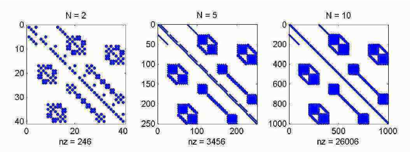
Figure 3.5: Example of matrix representation of the Liouvillean for the TDQS. The Hilbert space of the harmonic oscillator has dimension respectively $N=2,5,10$ ($nz$ is the number of no-zero elements of the mtrix). The non-zero elements are represented by a blue dot. The exponentials of position operator present in the tunneling amplitudes make the Liouvillean non-sparse (large squares progressively emerging in the figures from left to right). For large $N$ the SVD is not viable and we use the Arnoldi iteration scheme to find the null space of the Liouvillean.

Chapter 4 Wigner function distribution

The shuttle dynamics has, especially in the single dot device, an appealing simple classical interpretation and one can say that the name itself of “shuttle” suggests the idea of sequential and periodical loading, mechanical transport and unloading of electrons between a source and a drain lead. Semiclassical models typically treat the mechanical degree of freedom classically combined with incoherent sequential tunneling of electrons between leads and oscillating dot [1, 2, 3, 4, 5]. Motivated by the small size of the oscillations of a nanoscale shuttle, and thus by the possibility to observe signatures of quantum dynamics of the mechanical degree of freedom, we decided, following the suggestion of Armour and MacKinnon [7], to explore the model with a quantized oscillator. Nevertheless we also wanted to keep as much as possible the intuitive classical picture and to handle the quantum-classical correspondence. The Wigner function distribution seemed to us a good answer to all these requirements. It allows a clear visualization of the numerical results obtained within the framework of the GME and it shows in its equation of motion (the Klein-Kramers equation) an explicit quantum-classical correspondence (expansion in powers of $\hbar$) [34].

4.1 A quantum phase-space distribution

The concept of a probability distribution in phase space is problematic in quantum mechanics due to the uncertainty principle. It is not clear for example the meaning of the probability that a particle has a well defined position and momentum at a certain time and thus it seems difficult to define a probability distribution for such “non-observable events”. Nevertheless one can demonstrate that it is possible to associate with a state defined by a density operator $\rho(t)$ a unique function $P(q,p,t)$ on the phase space $(q,p)\times[t_{0},\infty)$ that satisfies some desirable properties. We list the required properties as stated by Hillary et al. in the review “Distribution functions in Physics: fundamentals” [34]:

1. $P(q,p,t)$ should be real;

2. $P(q,p,t)$ should reduce to a probability distribution once the conjugate variable is integrated:

   $$\begin{split}&\int dp\,P(q,p,t)=\langle q|\rho(t)|q\rangle\\ &\int dq\,P(q,p,t)=\langle p|\rho(t)|p\rangle\\ \end{split}$$ (4.1)

   and thus $P(q,p)$ is normalized

   $$\int dp\int dq\,P(q,p,t)=1$$ (4.2)

3. $P(q,p,t)$ should be Galilei invariant;

4. $P(q,p,t)$ should be invariant under space and time reflection;

5. In the force free case $P(q,p,t)$ should obey the classical equation of motion:

   $$\frac{\partial P}{\partial t}=-\frac{p}{m}\frac{\partial P}{\partial q}$$ (4.3)

6. If $P_{1}(q,p,t)$ and $P_{2}(q,p,t)$ are the distributions corresponding to the states $\rho_{1}(t)$ and $\rho_{2}(t)$ the following relation should hold:

   $$\int dq\langle q|\rho_{1}\rho_{2}|q\rangle=2\pi\hbar\int dq\int dp\,P_{1}(q,p,t)P_{2}(q,p,t)$$ (4.4)

Condition 6 is a requirement that comes from quantum mechanical considerations as can be seen from the following consequences. Assume $\rho_{1}=\rho_{2}=\rho$ being statistical mixtures of pure states $\rho_{\alpha}$ with weights $w_{\alpha}$

$$\rho=\sum_{\alpha}w_{\alpha}\rho_{\alpha}$$ (4.5)

and $P(q,p,t)$ the associated distribution, then from condition 6 we get

$$\int dq\int dp[P(q,p,t)]^{2}=\frac{\sum_{\alpha}w_{\alpha}^{2}}{2\pi\hbar}$$ (4.6)

This relation is discarding any too peacked distribution. In particular the classical distribution $P(q,p,t)=\delta(q-q_{0}(t))\delta(p-p_{0}(t))$ does not fulfill condition 6. If we assume now that $\rho_{1}$ and $\rho_{2}$ are pure states associated with orthogonal vectors, then:

$$\int dq\int dpP_{1}(q,p,t)P_{2}(q,p,t)=0$$ (4.7)

which implies that the two distributions are not positive everywhere. For this reason the distribution we are axiomatically constructing will take the name of quasi-probability distribution.

The distribution function that satisfy properties (1-5) or (1-4 and 6) exists unique [35], is defined as

$$W(q,p,t)=\frac{1}{2\pi\hbar}\int_{-\infty}^{+\infty}\!\!\!d\xi\left\langle q-\frac{\xi}{2}\right|\rho(t)\left|q+\frac{\xi}{2}\right\rangle\exp\left(\frac{ip\xi}{\hbar}\right)$$ (4.8)

and is commonly called Wigner distribution. The parallel with classical mechanics can be pushed even further associating to every observable on the Hilbert space the corresponding Wigner function:

$$A(q,p)=\int_{-\infty}^{+\infty}\!\!\!d\xi\left\langle q-\frac{\xi}{2}\right|A\left|q+\frac{\xi}{2}\right\rangle\exp\left(\frac{ip\xi}{\hbar}\right)$$ (4.9)

Two important relations can be derived from the definitions (4.8) and (4.9).

1. The trace of an operator in proportional to the integral on the phase space of its corresponding Wigner function:

   $${\rm Tr}A=\frac{1}{2\pi\hbar}\int dq\int dp\,A(q,p)$$ (4.10)

2. Given two operators $A$ and $B$ and the associate Wigner functions $A(q,p)$ and $B(q,p)$, the Wigner function associated to the product of the two operators $F=AB$ reads [35]:

$$F(q,p)=A(q,p)\exp\left(\frac{\hbar\Lambda}{2i}\right)B(q,p)$$ (4.11)

where $\Lambda$ is the differential operator:

$$\Lambda=\frac{\overleftarrow{\partial}}{\partial p}\frac{\overrightarrow{\partial}}{\partial q}-\frac{\overleftarrow{\partial}}{\partial q}\frac{\overrightarrow{\partial}}{\partial p}$$ (4.12)

The arrows indicate in which direction the derivative should be taken. A better insight in the expression (4.11) is given by the expansion of the exponential. Up to the first two terms it reads:

$$\begin{split}F(q,p)=&A(q,p)B(q,p)\\ +&\frac{\hbar}{2i}\left(\frac{\partial A}{\partial p}\frac{\partial B}{\partial q}-\frac{\partial A}{\partial q}\frac{\partial B}{\partial p}\right)\\ +&\left(\frac{\hbar}{2i}\right)^{2}\left(\frac{\partial^{2}A}{\partial p^{2}}\frac{\partial^{2}B}{\partial q^{2}}-2\frac{\partial^{2}A}{\partial p\partial q}\frac{\partial^{2}B}{\partial q\partial p}+\frac{\partial^{2}A}{\partial q^{2}}\frac{\partial^{2}B}{\partial p^{2}}\right)\\ +&\left(\frac{\hbar}{2i}\right)^{3}\ldots\end{split}$$ (4.13)

The expansion shows the power of the formalism to treat the quantum-classical correspondence: given a length, a mass, and a time scale for the system we can rescale the coordinates and the expansion will appear as an expansion in $\hbar/S_{\rm sys}$ where $S_{\rm sys}$ is the typical action of the system. Classical systems have a large action $S_{sys}\gg\hbar$ and only the first term in the expansion is relevant. In the opposite limit $S_{sys}\approx\hbar$ the full expansion should be considered. We have now the tools to translate into the Wigner formalism the expression for the expectation value of an operator: We start from the definitions:

$$\langle A(t)\rangle\equiv{\rm Tr}\{\rho(t)A\}=\int dq\int dp\,W(q,p,t)\exp\left(\frac{\hbar\Lambda}{2i}\right)A(q,p)$$ (4.14)

Inserting the expansion in $\hbar$ of the exponential and using the regularity of the Wigner distribution at infinity we obtain the “classical” result:

$$\langle A(t)\rangle=\int dq\int dp\,W(q,p,t)A(q,p)$$ (4.15)

A second important consequence of the Groenewold equation (4.11) is the quantum-classical correspondence for the dynamics of the distribution function $W(q,p,t)$. In the Wigner formalism the equation of Liouville-von Neumann reads:

$$\frac{\partial W}{\partial t}=-\frac{i}{\hbar}\left[H\exp\left(\frac{\hbar\Lambda}{2i}\right)W-W\exp\left(\frac{\hbar\Lambda}{2i}\right)H\right]$$ (4.16)

where $H\equiv H(q,p)$ is the Wigner function associated with the Hamiltonian for the system. Due to the fact that the differential operator $\Lambda$ is odd with respect of the exchange of the two functions on which it is acting only odd powers of the expansion in $\hbar/S_{\rm sys}$ survive in (4.16). In the limit $\hbar/S_{\rm sys}\to 0$ we get the classical Liouville equation:

$$\frac{\partial W^{c}}{\partial t}=\{H,W^{c}\}_{P}$$ (4.17)

where $\{,\}_{P}\equiv\frac{\overleftarrow{\partial}}{\partial q}\frac{\overrightarrow{\partial}}{\partial p}-\frac{\overleftarrow{\partial}}{\partial p}\frac{\overrightarrow{\partial}}{\partial q}=-\Lambda$ are the Poisson brackets and the superscript $c$ indicates the classical limit for the Wigner distribution.

4.2 Klein-Kramers equations for the SDQS

With the knowledge acquired in the previous section we will now concentrate on the translation in the Wigner formalism of the GME for shuttle devices that we derived in the previous chapter. We concentrate only on the SDQS first because the technique is completely illustrated in this simpler case and also because contrary to the single dot device for the TDQS we will use the Wigner distribution only as a visualization tool. In the derivation of the GME for the single dot device (see §3.4.1) we identified three components of the Liouvillean super-operator:

$$\mathcal{L}=\mathcal{L}_{\rm coh}+\mathcal{L}_{\rm driv}+\mathcal{L}_{\rm damp}$$ (4.18)

distinguishing the coherent contribution that describes the evolution of the system without the electrical and mechanical baths from a driving contribution where the coupling to the leads is inserted and a damping term that takes into account the interaction with the dissipative environment of the mechanical degree of freedom. We separately treat their translation into the Wigner formalism in the following sections.

4.2.1 Coherent Liouvillean

We start recalling explicitly the action of the coherent part of the Liouvillean on the two non-vanishing electrical components of the reduced density matrix ($\sigma_{00}$ and $\sigma_{11}$):

$$\mathcal{L}_{\rm coh}\left(\begin{array}[]{c}\sigma_{00}\\ \sigma_{11}\end{array}\right)=-\frac{i}{\hbar}\left(\begin{array}[]{c}{[H_{\rm osc},\sigma_{00}]}\\ {[H_{\rm osc}-e\mathcal{E}x,\sigma_{11}]}\end{array}\right)$$ (4.19)

It is easy to verify from the definition (4.9) that for operators which are sum of functions of momentum or position operator only, the associated Winger functions coincide with the corresponding classical dynamical variables. For example the Wigner function of the oscillator Hamiltonian reads:

$$H_{\rm osc}(q,p)=\frac{p^{2}}{2m}+\frac{1}{2}m\omega^{2}q^{2}$$ (4.20)

and analogously the electrostatic component becomes $e\mathcal{E}q$.

As already mentioned the commutator structure of the Liouville-von Neumann equation implies that only the odd components of the $\hbar$ expansion of the Groenewold operator $\exp(\hbar\Lambda/2i)$ should be retained. Since the third order in the expansion contains already derivatives in $q$ and $p$ up to the third order, and the oscillator Hamiltonian is quadratic in $q$ and $p$ only the first order survives and the coherent part of the Liouvilliean acquires the classical form:

$$\mathcal{L}_{\rm coh}\left(\begin{array}[]{c}W_{00}\\ W_{11}\end{array}\right)=\left(\begin{array}[]{c}{m\omega^{2}q\frac{\partial W_{00}}{\partial p}-\frac{p}{m}\frac{\partial W_{00}}{\partial q}}\\ {m\omega^{2}(q-d)\frac{\partial W_{11}}{\partial p}-\frac{p}{m}\frac{\partial W_{11}}{\partial q}}\end{array}\right)$$ (4.21)

where the displacement $d=\frac{e\mathcal{E}}{m\omega^{2}}$ is the equilibrium position of the oscillator subject to a constant force $e\mathcal{E}$ and we have introduced a Wigner distribution for each of the electrical states of the system. In this charge resolved Wigner functions one can read the probability density for the quantum dot to have a specific position and (average) momentum when in a specific electrical state. In this way we can monitor the correlation between charge and position (momentum) of the oscillating dot, important to discriminate the shuttling regime from other transport regimes.

4.2.2 Driving Liouvillean

The driving term of the Liouvillean for the SDQS is a rate equation somehow modified to take into account the operator form of the position-dependent rates:

$$\mathcal{L}_{\rm driv}\left(\begin{array}[]{c}\sigma_{00}\\ \sigma_{11}\\ \end{array}\right)=\left(\begin{array}[]{c}-\frac{\Gamma_{L}}{2}\{e^{-2x/\lambda},\sigma_{00}\}+\Gamma_{R}e^{x/\lambda}\sigma_{11}e^{x/\lambda}\\ -\frac{\Gamma_{R}}{2}\{e^{2x/\lambda},\sigma_{11}\}+\Gamma_{L}e^{-x/\lambda}\sigma_{00}e^{-x/\lambda}\\ \end{array}\right)$$ (4.22)

where $\{A,B\}\equiv AB+BA$ is the anticommutator.

We calculate first the generic form of the symmetric component of the driving Liouvillian in the Wigner representation. It is easier in this case to start directly from the definition:

$$\begin{split}&\frac{1}{2\pi\hbar}\int_{-\infty}^{+\infty}\!\!\!d\xi\left\langle q-\frac{\xi}{2}\right|\Gamma_{L,R}e^{\mp x/\lambda}\sigma_{ii}(t)e^{\mp x/\lambda}\left|q+\frac{\xi}{2}\right\rangle\exp\left(\frac{ip\xi}{\hbar}\right)\\ =&\,\Gamma_{L,R}e^{\mp 2q/\lambda}\int_{-\infty}^{+\infty}\!\!\!d\xi\left\langle q-\frac{\xi}{2}\right|\sigma_{ii}(t)\left|q+\frac{\xi}{2}\right\rangle\exp\left(\frac{ip\xi}{\hbar}\right)\\ =&\Gamma_{L,R}e^{\mp 2q/\lambda}W_{ii}(q,p,t)\end{split}$$ (4.23)

where $i=0,1$ in accordance with the sign of the exponential respectively $-,+$ and the subscript $L,R$ in the tunneling rate $\Gamma$. Only the classical component contributes to this term since the Wigner representation is just the product of the three Wigner functions.

Quantum correction are present instead in the anticommutator component of the driving Liouvillean. Again we calculate the generic form :

$$\begin{split}&-\frac{1}{2\pi\hbar}\int_{-\infty}^{+\infty}\!\!\!d\xi\left\langle q-\frac{\xi}{2}\right|\frac{\Gamma_{L,R}}{2}\{e^{\mp 2x/\lambda},\sigma_{ii}(t)\}\left|q+\frac{\xi}{2}\right\rangle\exp\left(\frac{ip\xi}{\hbar}\right)\\ =&\,-\frac{\Gamma_{L,R}}{2}\left[e^{\mp 2q/\lambda}\exp\left(\frac{\hbar\Lambda}{2i}\right)W_{ii}(q,p,t)+W_{ii}(q,p,t)\exp\left(\frac{\hbar\Lambda}{2i}\right)e^{\mp 2q/\lambda}\right]\\ =&-\Gamma_{L,R}e^{\mp 2q/\lambda}\sum_{n=0}^{\infty}\frac{1}{(2n)!}\left(\frac{\hbar\Lambda}{2i}\right)^{2n}W_{ii}(q,p,t)\\ =&-\Gamma_{L,R}e^{\mp 2q/\lambda}\sum_{n=0}^{\infty}\frac{(-1)^{n}}{(2n)!}\left(\frac{\hbar}{\lambda}\right)^{2n}\frac{\partial^{2n}}{\partial p^{2n}}W_{ii}(q,p,t)\end{split}$$ (4.24)

where because of the symmetry of the anticommutator only even powers of the Groenewold operator give non vanishing contributions (line 2 to 3 in (4.24) ) and they are equal for both terms of the anticommutator. In the last line we appreciate the control parameter for the quantum-classical correspondence. Especially in the shuttling regime the typical length, mass and time scales of the system are the tunneling length $\lambda$ and the harmonic oscillator mass $m$ and inverse frequency $1/\omega$. Rescaling the phase space coordinates to the adimensional $X=q/\lambda$ and $P=p/(m\omega\lambda)$ we obtain the expansion parameter:

$$\frac{\hbar}{m\omega\lambda^{2}}=2\left(\frac{\Delta x_{z}}{\lambda}\right)^{2}$$ (4.25)

that is the ratio between the zero point fluctuation of the oscillator position ($\Delta x_{z}$) and the tunneling length ($\lambda$). The bigger $\lambda$ the more classical is the behavior of the harmonic oscillator.

All together the driving Liouvillean in the Wigner representation takes the form:

$$\mathcal{L}_{\rm driv}\left(\begin{array}[]{c}W_{00}\\ W_{11}\end{array}\right)=\left(\begin{array}[]{c}{\Gamma_{R}e^{2q/\lambda}W_{11}-\Gamma_{L}e^{-2q/\lambda}\sum_{n=0}^{\infty}\frac{(-1)^{n}}{(2n)!}\left(\frac{\hbar}{\lambda}\right)^{2n}\frac{\partial^{2n}}{\partial p^{2n}}W_{00}}\\ {\Gamma_{L}e^{-2q/\lambda}W_{00}-\Gamma_{R}e^{2q/\lambda}\sum_{n=0}^{\infty}\frac{(-1)^{n}}{(2n)!}\left(\frac{\hbar}{\lambda}\right)^{2n}\frac{\partial^{2n}}{\partial p^{2n}}W_{11}}\end{array}\right)$$ (4.26)

4.2.3 Damping Liouvillean

The damping Liouvillean is identical for the two electrical components of the reduced density matrix and we give a unified derivation of the corresponding Wigner formulation. In terms of density matrices it reads:

$$\mathcal{L}_{\rm damp}(\sigma)=-\frac{i\gamma}{2\hbar}[x,\{p,\sigma\}]-\frac{\gamma m\omega}{2\hbar}(2n_{B}+1)[x,[x,\sigma]]$$ (4.27)

Once again we apply the Groenewold modified product (4.11) to obtain the Wigner formulation. Since the damping Liouvillean is quadratic in the operators $x$ and $p$ we expect only the first two terms of the expansion in the operator $\Lambda$ to contribute.

$$\mathcal{L}_{\rm damp}W=\gamma\frac{\partial}{\partial p}pW+\gamma m\hbar\omega\left(n_{B}+\frac{1}{2}\right)\frac{\partial^{2}}{\partial p^{2}}W$$ (4.28)

The term of first order in the derivative is called damping term while the second diffusion term. One way to understand the meaning of this names is to derive this equation for the distribution function starting from the corresponding Langevin equations describing the brownian motion of a particle in an harmonic potential:

$$\begin{split}\dot{x}&=\frac{p}{m}\\ \dot{p}&=-m\omega^{2}x-\gamma p+\xi(t)\end{split}$$ (4.29)

The first term in the RHS of equation (4.28) is related to the velocity dependent friction ($-\gamma p$) while the second comes from the stochastic force $\xi(t)$. The analogy with classical brownian motion can be pushed even further considering the rescaling:

$$X=\frac{x}{\ell},\qquad P=\frac{p}{m\omega\ell}$$ (4.30)

where $\ell=\sqrt{\frac{\hbar}{2m\omega}(2n_{B}+1)}$. The damping Liouvillian in terms of the rescaled variables reads:

$$\mathcal{L}_{\rm damp}(W)=\gamma\frac{\partial}{\partial P}\left(P+\frac{\partial}{\partial P}\right)\,W$$ (4.31)

and only the scaling distinguishes the quantum from the classical description While in the low temperature limit $2n_{B}\ll 1$ and the length scale $\ell$ tends to the oscillator zero point fluctuation $\Delta x_{z}$, in the high temperature limit $\hbar$ drops out from the equations and $\ell$ is given by the the thermal length $\lambda_{th}=\sqrt{\frac{k_{B}T}{m\omega^{2}}}$.

Finally we collect the results of the previous sections and write the equation of motion for the SDQS in the Wigner function formulation:

$$\frac{\partial W_{00}}{\partial t}=$$

(4.32)

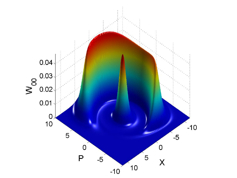
Figure 4.1: Example of 3-D visualization of the stationary solution of the Klein-Kramers equations for the SDQS. The surface represents the quasi-probability distribution of the empty dot $W^{stat}_{00}(q,p)$. Coordinate and momentum are expressed in adimensional units: $X=q/x_{0}$ and $P=px_{0}/\hbar$, where $x_{0}=\sqrt{\hbar/(m\omega)}$. The distribution shows two distinct features. The probability is high near the origin of the phase space and represents the oscillator in the ground state. The other structure corresponds to the part of the limit cycle drawn by the empty dot in the shuttling regime.

Chapter 5 Investigation tools

The dynamics of the shuttling devices or at least of the simplified models for them that we consider, is all contained in the GMEs for the reduced density matrices (3.120) and (3.131) or in the corresponding Klein-Kramers equations for the Wigner distributions (e.g. equation (4.32) for the SDQS). The coupling to the continuum of states in the electrical and mechanical baths introduces irreversibility in the system and its statistical properties (represented by the reduced density matrix or Wigner distribution) tend to a stationary limit. This does not mean that the system itself is in a static condition. In particular an electric current sustained by the bias always flows through the device driving the movable dot into a variety of different dynamical regimes. In order to analyze the properties of these different operating conditions of the electronic shuttles we use three investigation tools. We study the phase space distribution functions associated with the stationary solution of the GME, the corresponding current and the current-noise, taking as control parameters the damping rate of the mechanical degree of freedom, or the gate voltage of the different dots, or the injection and ejection rates. Through the phase-space analysis or the current and noise calculation we gain somehow complementary information about the system. These approaches are described in detail in the next three sections.

5.1 Phase space distributions: dots, rings and bananas

The phase space analysis of the shuttle dynamics is based on the Wigner representation of the stationary solution of the GME:

$$W_{ij}^{\rm stat}(q,p)=\frac{1}{2\pi\hbar}\int_{-\infty}^{+\infty}\!\!\!d\xi\left\langle q-\frac{\xi}{2}\right|\sigma_{ij}^{\rm stat}\left|q+\frac{\xi}{2}\right\rangle\exp\left(\frac{ip\xi}{\hbar}\right)$$ (5.1)

where the subscript $ij$ indicates the electrical state that we are considering. Since typically we are not interested in coherencies between electronic states we set $i=j$ and the resulting Wigner distribution represents the joint probability for the system to be in the specific mechanical state $(q,p)$ and electrical state $i$. The total Wigner distribution

$$W^{\rm stat}_{\rm tot}(q,p)=\sum_{i}W^{\rm stat}_{ii}(q,p)$$ (5.2)

where the sum is extended to all the electrical states of the system, gives information about the mechanical state independently from the electronic state of the device.

5.1.1 Shuttling instability

For the SDQS we analyze first the behavior of the Wigner distribution as a function of the mechanical damping. The mechanical dynamics shows a typical feature qualitatively independent from the other parameters of the model. At high damping rates the total Wigner distribution is concentrated around the origin of the phase space and represents the harmonic oscillator in the ground state. While reducing the mechanical damping a ring progressively develops and the central “dot” eventually disappears (Fig. 5.1). We interpret the ring as a smeared limit cycle trajectory: by reducing the damping the equilibrium position becomes unstable and a stable limit cycle develops. The threshold for this transition is given by the effective tunneling rates of the electrons.

This interpretation is represented in the following picture: every time an electron jumps on the movable grain the latter is subject to the electrostatic force $e\mathcal{E}$ that accelerates it towards the right. Energy is pumped into the mechanical system and the dot starts to oscillate. If the damping is high compared to the tunneling rates the oscillator dissipates this energy into the environment before the next tunneling event: on average the dot remains in its ground state. On the contrary for very small damping the relaxation time of the oscillator is long and multiple “forcing events” happen before the relaxation takes place. This continuously drives the oscillator far from equilibrium and a stationary state is reached only when the energy pumped per cycle into the system is dissipated during the same cycle in the environment.

It is not difficult to realize that, like for a macroscopic swing, in order to sustain the motion one needs coordination between forcing (here related to the electrical dynamics) and oscillations. This coordination is revealed by the charge resolved Wigner distributions $W_{00}$ and $W_{11}$. The ring that appears in the total distribution is asymmetrically shared by the empty and charged-dot distributions (Fig. 5.1).

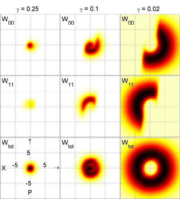
Figure 5.1: Phase space picture of the tunneling-to-shuttling crossover. The respective rows show the Wigner distribution functions for the discharged ($W_{00}$), charged ($W_{11}$) and sum ($W_{\rm tot}$) states of the oscillator in the phase space (horizontal axis–coordinate in units of $x_{0}=\sqrt{\hbar/(\hbar\omega)}$, vertical axis – momentum in $\hbar/x_{0}$). The values of the parameters are: $\lambda=x_{0}$, $T=0$, $d=0.5x_{0}$, $\Gamma=0.05\omega$. The values of $\gamma$ are in units of $\omega$. The Wigner functions are normalized within each column.

The Wigner distributions reveal the charge-position (momentum) correlation typical of the shuttling regime: for negative displacements and positive momentum (i.e. leaving the source lead) the dot is prevalently charged while it is empty for positive displacements and negative momentum (coming from the drain lead). Self-sustained mechanical oscillations and shuttling electron transport are part of the same phenomenon.

5.1.2 Classical vs. Quantum Shuttle

The instability we showed in the previous section was predicted already by Gorelik et al. [1] (even if as a function of the external bias) in the form of a sharp transition between an equilibrium and a limit cycle dynamics of the oscillator and is called shuttle instability. The quantum mechanical description of the harmonic oscillator that we give introduces two effects in the model: it smears the transition into a crossover and reveals the possibility to trigger the shuttling regime even at zero electric field [8] when classically the electrical and mechanical dynamics would be decoupled and the device would behave as a damped harmonic oscillator that with no feedback influences a single electron transistor (Fig. 5.2).

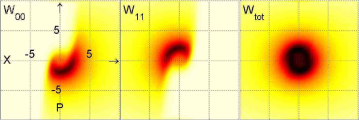
Figure 5.2: Shuttling at zero electric field. The three Wigner distributions for the empty, charged, and sum states are represented in the usual adimensional phase space $(X,P)$ (see Fig. 5.1). The parameter values are $\lambda=x_{0}$, $T=0$, $d=0$, $\Gamma=0.05\omega$, $\gamma=0$.

The amplitude of the shuttling oscillations of the quantum dot is also dependent on the tunneling length and bare injection rate. In particular it grows with the tunneling length $\lambda$ and with the inverse of the bare injection rate.

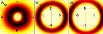
Figure 5.3: Transition from “quantum” to “classical” shuttling. The figure shows the total Wigner function for three different sets of parameters. We keep constant damping ($\gamma=0.02\omega$) temperature ($T=0$) and electric field ($d=0.5x_{0}$) and change the injection rate and tunneling length. From left to right respectively: $(\Gamma=0.05\omega,\,\lambda=x_{0})$, $(\Gamma=0.05\omega,\,\lambda=2x_{0})$, $(\Gamma=0.01\omega,\,\lambda=2x_{0})$.

This behavior can be understood as a self-consistent compensation to accomplish the non-adiabatic condition that the effective injection rate $\bar{\Gamma}$ must be comparable in the shuttling regime with the oscillator frequency $\omega/2\pi$. The larger the amplitude of the oscillation the more classical is the behavior of the harmonic oscillator. This concept can be understood also from a geometric point of view: the ring gets closer and closer to a circle since the width, given by the amount of thermal and shot noise remains constant (or decreases as we will see in the coexistence regime semianalytics) while the diameter increases. Another natural parameter that reveals this quantum to classical transition is the ratio between $\hbar$ and the area enclosed by the ring. This tends to zero in the classical limit (Fig. 5.3).

5.1.3 Different electronic processes in the TDQS

The Wigner distribution analysis of the TDQS is performed in analogy with the SDQS on the states corresponding to the empty and charged central dot. Namely we consider:

$$\begin{split}W_{UU}^{\rm stat}(q,p)&=\frac{1}{2\pi\hbar}\int_{-\infty}^{+\infty}\!\!\!d\xi\left\langle q-\frac{\xi}{2}\right|\sigma_{00}^{\rm stat}+\sigma_{LL}^{\rm stat}+\sigma_{RR}^{\rm stat}\left|q+\frac{\xi}{2}\right\rangle\exp\left(\frac{ip\xi}{\hbar}\right)\\ W_{CC}^{\rm stat}(q,p)&=\frac{1}{2\pi\hbar}\int_{-\infty}^{+\infty}\!\!\!d\xi\left\langle q-\frac{\xi}{2}\right|\sigma_{CC}^{\rm stat}\left|q+\frac{\xi}{2}\right\rangle\exp\left(\frac{ip\xi}{\hbar}\right)\end{split}$$ (5.3)

As suggested by the work of Armour and MacKinnon [7] we consider as control parameter the difference between the gate voltages on the left and right dot (the so-called device bias $\Delta V$). It was found in [7] that the triple dot system exhibits different regimes of transport at different device biases. The current peaks at $\Delta V\approx n\hbar\omega$ were identified as effects of electromechanical resonances within the device. Yet, the different peaks may correspond to different physical mechanisms – while the peak around $\Delta V\approx\hbar\omega$ is mainly due to the incoherent oscillator-assisted tunneling the peak at $\Delta V\approx 2\hbar\omega$ reveals a clear shuttling component. This finding by Armour and MacKinnon based on indirect evidence of parametric dependencies of the current curves (e.g. the dependence of the current curve on the tunneling length $\lambda$) is confirmed by the direct inspection of the phase space distribution (Fig. 5.4). The half-moon-like shape characteristic for the shuttling transport is only present around $\Delta V\approx 2\omega$ while all other plots show just the fuzzy spot indicative of incoherent tunneling. However, our direct criterion for detecting the shuttling regime reveals a close similarity between the resonances. For increasing injection rate we can see that the shuttling regime gradually sets in also in the vicinity of the first resonance peak. This reveals the cross over character of the onset of the shuttling instability found also for the SDQS.

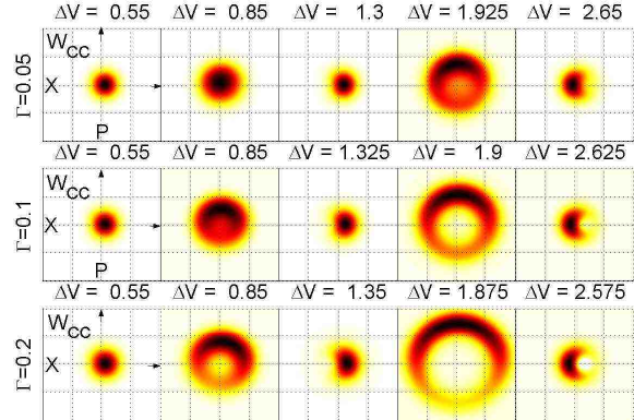
Figure 5.4: Wigner distributions for the central dot in the charged state. The half-moon shuttling signature, always present at the second resonance ($\Delta V\approx 2\hbar\omega$) progressively emerges also in the first resonance ($\Delta V\approx\hbar\omega$). The other parameters are $V_{0}=0.757\hbar\omega,\,\lambda=5\Delta x_{z},\,x_{0}=7.071\Delta x_{z},\,\gamma=0.0125\omega$.

As can be seen in more detail in the work by C. Flindt et al. [33] and in the Master thesis by C. Flindt [12] the TDQS exhibits at higher device biases another transport mechanism that competes with the shuttling transport. For $\Delta V\approx 3\omega,4\omega$ inelastic co-tunneling takes place and a clear signature of this phenomenon can be seen in the vanishing of the charged central dot Wigner function (see Fig. 5 in [33]).

5.2 Current

The Wigner distribution functions are a very clean theoretical tool to investigate the dynamical properties of shuttle devices, but unfortunately it seems very difficult (if not impossible) to access experimentally these functions. For this reason, with in mind the distribution function description, we investigate the electronic transport properties in the shuttle devices (more realistically measurable) starting with the stationary current.

5.2.1 Calculation of the stationary current

We already encountered in section 3.3.5 the definition of right and left lead currents:

$$\begin{split}I_{R}(t)&=\dot{N}_{R}(t)\\ I_{L}(t)&=\dot{N}_{L}(t)\end{split}$$ (5.4)

where $N_{R}(t)$ ($N_{L}(t)$) are the total number of electrons (holes) collected in the right (left) lead at time $t$. We have also related these functions to the elements of the $n$($h$)-resolved density matrix and corresponding GME (Eq. (3.54) and (3.56)). Since we are interested exclusively in the stationary current we analyze now in detail only the electron current in the right lead in presence of a shuttle device (SDQS or TDQS). The total number of electrons collected in the right lead $N_{R}(t)$ can be written as:

$$N_{R}(t)=\sum_{n=0}^{\infty}nP_{n}(t)$$ (5.5)

where $P_{n}(t)$ is the probability for $n$ electrons to be collected into the right lead at time $t$. We express the probability $P_{n}(t)$ as the trace of the $n$-resolved reduced density matrix over the system degrees of freedom:

$$P_{n}(t)={\rm Tr}_{\rm sys}\left\{\sigma^{(n)}(t)\right\}={\rm Tr}_{\rm osc}\left\{\textstyle{\sum_{i}}\sigma_{ii}^{(n)}(t)\right\}$$ (5.6)

where $i$ is the electrical state of the device: and in the SDQS $i=0,1$ while in the TDQS $i=0,L,C,R$. The $n$-resolved GME ($n$-GME) comes now into play and the current is expressed as a function of $\sigma_{ii}^{(n)}(t)$:

$$\begin{split}I_{R}(t)&=\sum_{n=0}^{\infty}\sum_{i}n{\rm Tr}_{\rm osc}\left\{\dot{\sigma}_{ii}^{(n)}(t)\right\}\\ &=\sum_{n=0}^{\infty}n\sum_{i}{\rm Tr}_{\rm osc}\left\{\mathcal{L}_{\rm coh}\big{[}\sigma^{(n)}(t)\big{]}_{ii}+\mathcal{L}_{\rm driv}\big{[}\sigma(t)\big{]}^{(n)}_{ii}+\mathcal{L}_{\rm damp}\big{[}\sigma^{(n)}_{ii}(t)\big{]}\right\}\end{split}$$ (5.7)

where we have implicitly specified with the position of the square parentheses the different components of the density matrix addressed by the different Liouvilleans.

We calculate first the SDQS right (particle) current. The coherent and damping part of the Liouvillean have a commutator structure (see Eq. (3.116)) and vanish under trace. We are left with the contribution given by the driving Liouvillean:

$$I_{R}(t)={\rm Tr}_{\rm osc}\left\{\Gamma_{R}e^{2x/\lambda}\sum_{n=0}^{\infty}n\left[\sigma_{11}^{(n-1)}(t)-\sigma_{11}^{(n)}(t)\right]\right\}$$ (5.8)

where we have used the cyclic property of the trace to evaluate the sum over the two electrical components. The particular ordering of the position dependent injection and ejection operators $\Gamma_{L,R}(x)$ is irrelevant under trace and the sum over the number of electron in the resevoir is formally identical to the one obtained for the static single dot (see Eq. (3.54)). We evaluate it and obtain:

$$I_{R}(t)={\rm Tr}_{\rm osc}\left\{\Gamma_{R}e^{2x/\lambda}\sigma_{11}(t)\right\}$$ (5.9)

With completely analogous arguments one derives the expression for the left current:

$$I_{L}(t)={\rm Tr}_{\rm osc}\left\{\Gamma_{L}e^{-2x/\lambda}\sigma_{00}(t)\right\}$$ (5.10)

The stationary current is obtained by substituting in (5.9) or (5.10) the stationary solution $\sigma^{\rm stat}$ of the GME. It is interesting that the stationary particle current is written as the average injection (ejection) rate:

$$I^{\rm stat}=\begin{array}[]{c}\nearrow\\ \searrow\end{array}\begin{array}[]{c}{\rm Tr}_{\rm osc}\left\{\Gamma_{R}e^{2x/\lambda}\sigma^{\rm stat}_{11}\right\}={\rm Tr}_{\rm sys}\left\{\Gamma_{R}(x)|1\rangle\!\langle 1|\sigma^{\rm stat}\right\}=\bar{\Gamma}_{R}\\ \\ \\ {\rm Tr}_{\rm osc}\left\{\Gamma_{L}e^{-2x/\lambda}\sigma^{\rm stat}_{00}\right\}={\rm Tr}_{\rm sys}\left\{\Gamma_{L}(x)|0\rangle\!\langle 0|\sigma^{\rm stat}\right\}=\bar{\Gamma}_{L}\end{array}\begin{array}[]{c}\searrow\\ \nearrow\end{array}=\bar{\Gamma}$$ (5.11)

where we have introduced the projectors $|1\rangle\!\langle 1|\equiv c_{1}^{{\dagger}}c_{1}^{\phantom{\dagger}}$ and $|0\rangle\!\langle 0|\equiv 1-c_{1}^{{\dagger}}c_{1}^{\phantom{\dagger}}$ on the electronic Hilbert space and we calculate the average injection and ejection rates taking into account Coulomb blockade and the single level structure. Namely the injection (ejection) rate average is calculated only on system states with empty (charged) dot. A special remark concerns correlations: the shuttling regime is characterized by strong electromechanical correlations and they should be recorded in the current since in general:

$$I^{\rm stat}={\rm Tr}_{\rm sys}\{\Gamma_{L}(x)|0\rangle\!\langle 0|\sigma^{\rm stat}\}\neq{\rm Tr}_{\rm sys}\{\Gamma_{L}(x)\sigma^{\rm stat}\}{\rm Tr}_{\rm sys}\{|0\rangle\!\langle 0|\sigma^{\rm stat}\}$$ (5.12)

5.2.2 Current characteristics of the SDQS

We study the current as a function of the mechanical damping. The results for different values of the bare injection (ejection) rate and of the tunneling length are presented in Fig. 5.5. At low damping the current saturates, independently from the value of the other parameters, at the “magic” value $I\approx 0.16\omega$ (numerical approximation of the frequency of the harmonic oscillator $\omega/2\pi$). Increasing the damping the stationary current drops, more or less rapidly, to a plateau, dependent this time on both the bare tunneling rate and length. Further increase of the damping does not change the scenario. The transition between the plateau and the saturation point is faster the more “classical” the other parameters are (i.e. small injection rate and large tunneling length).

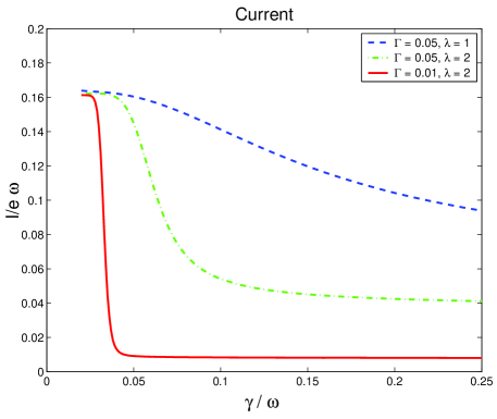
Figure 5.5: Particle stationary current of the SDQS plotted as a function of the damping rate. The bare electronic rate $(\Gamma)$ is given in units of the oscillator frequency. The tunneling length is given in units of $x_{0}=\sqrt{\hbar/m\omega}$. The current and the damping rate are expressed in adimensional units also by rescaling with the oscillator frequency $\omega$. The saturation of the current to the limit of one electron per cycle characteristic of the shuttling regime at low damping is visible. The transition to the the high damping limit (oscillator in ground state) gets sharper the more classical is the dynamics as is indicated also by the parameters (see text for explanation).

If we compare the current results with the Wigner function distribution we can recognize a correspondence between the shuttling charge-position (momentum) correlation and the saturation point, as well as a progressive disappearing of the ring structure in correspondence with the current transition. The high damping plateau in the current sets in when the mechanical oscillator lays into its ground state and the Wigner distribution function is reduced to a fuzzy spot close to the origin of the phase space (Fig. 5.6).

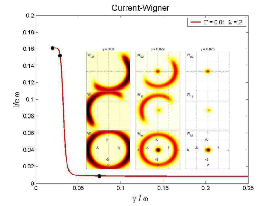
Figure 5.6: Most “classical” current-damping curve. The Wigner function distributions in the insets correspond to the three dots indicated on the curve and show how the transition looks like in the phase space.

5.2.3 Electromechanical resonances of the TDQS

The calculation of the TDQS stationary current follows the same argument line we adopted for the SDQS. Also the analytic expression shares essentially the same structure, the only difference being the projector that appears in the right lead current and the tunneling rate that in this case is not position dependent. The electrons tunnel to the resevoir only from the right dot and the current reads:

$$I_{R}^{\rm stat}=\Gamma_{R}{\rm Tr}_{\rm osc}\left\{\sigma^{\rm stat}_{RR}\right\}=\Gamma_{R}{\rm Tr}_{\rm sys}\left\{|R\rangle\!\langle R|\sigma^{\rm stat}\right\}=\bar{\Gamma}_{R}$$ (5.13)

Since there are not position operators in the left or right lead current one could argue that the stationary current of the TDQS do not record signs of charge-position correlation. The solution to this problem comes from the structure of the device. Instead of looking at the system-lead tunneling current one can concentrate on the tunneling current within the device: in the stationary limit charge conservation ensures they are equal. For example the left-center current reads in the stationary limit:

$$I_{LC}^{\rm stat}={\rm Tr}_{\rm osc}\{it_{L}(x)(\sigma^{\rm stat}_{CL}-\sigma^{\rm stat}_{LC})\}$$ (5.14)

as can be derived tracing the second equation of (3.131).

A detailed analysis of the current in the TDQS with the device bias as control parameter can be found in the work by Armour and MacKinnon [7]. Extension and analysis of the same model in other parameter regimes are given in [11] and extensively in [12] and [33]. Qualitatively we can describe the current-device bias characteristics as series of peaks (electromechanical resonancies) at $\Delta V\approx n\hbar\omega$. It is difficult to establish only from the analysis of the current the nature of these peaks. Armour and MacKinnon have an interpretation of the different mechanisms underlying these resonances based on the analysis of the spectrum of the decoupled three dot device + harmonic oscillator. This method can visualize very well the basic mechanisms of elastic or inelastic phonon assisted tunneling. Other information can be gained from the behaviour of the current at different resonances as a function of the tunneling length or mechanical damping. We acknowledge the validity of this analysis but we also think that an independent source of information (such as the phase space or the current-noise) is needed to discriminate directly between different operating regimes. In Fig. 5.7 we report a set of current curves in which one can recognize the first three electromechanical resonances.

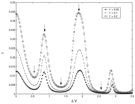
Figure 5.7: Current as function of device bias in TDQS. Different curves correspond to different injection rates $\Gamma$. The particle current and the injection rate $\Gamma$ are scaled with the mechanical frequency $\omega$. The first three electromechanical resonances are visible. The arrows indicate points of minimum or maximum current and the corresponding Wigner distributions are reported in Fig. 5.4. The other parameters are $V_{0}=0.757\hbar\omega,\,\lambda=5\Delta x_{z},\,x_{0}=7.071\Delta x_{z},\,\gamma=0.0125\omega$.

The temperature influences the device characteristics in different ways since different competing transport mechanisms (phonon assisted-tunneling, co-tunneling, shuttling) depend on temperature in very different ways. A generic feature can though be recognized: at finite temperature electromechanical resonances are found also at negative device biases (see for example Fig. 2 in [33]) when electrons can tunnel through the device only by gaining energy from the oscillator. This observation suggests the idea of an active phonon cooling device useful to prepare for example a macroscopic harmonic oscillator close to its quantum ground state more efficiently than by coupling it to a “very cold” thermal resevoir.

5.3 Current noise

An unequivocal experimental observation of the shuttling transition has not yet been achieved. The IV-curve measured in recent experiments on a vibrating ${\rm C_{60}}$ can be interpreted in terms of shuttling [19], but also alternative explanations have been promoted [20, 21, 36]. It is therefore natural to look for more refined experimental tools than just the average current through the device. An obvious candidate is the current noise spectrum [37, 38]. The measurement of the noise spectrum or even higher moments (full counting statistics) reveals more information about the transport through the device than just the mean current. The theoretical studies of the noise have attracted much attention recently in NEMS in general [39, 40, 41] as well as for the shuttling set up [5, 42, 14] in the (semi)classical limit. The quantum mechanical theory for shot noise in NEMS that we treat here is also exposed in [23] and in a more general form in [33] and is mainly due to T. Novotný in collaboration with the author and C. Flindt.

5.3.1 The MacDonald formula

Let us consider the (particle) current flowing from the dot to the right lead of the SDQS. This is defined (in the Heisenberg picture) as the time derivative of the number operator of the right lead:

$$\begin{split}\hat{I}_{R}(t)&=\dot{\hat{N}}_{R}(t)=-\frac{i}{\hbar}[\hat{H}(t),\hat{N}_{R}(t)]\\ &=-\frac{i}{\hbar}\hat{T}_{r}(\hat{x})\sum_{k}\left(\hat{c}^{{\dagger}}_{r_{k}}\hat{c}^{\phantom{\dagger}}_{1}+\hat{c}^{{\dagger}}_{1}\hat{c}^{\phantom{\dagger}}_{r_{k}}\right)\end{split}$$ (5.15)

where

$$N_{R}=\sum_{k}c^{{\dagger}}_{r_{k}}c^{\phantom{\dagger}}_{r_{k}},$$ (5.16)

the symbol $\hat{\bullet}$ indicates the Heisenberg picture and $H$ is the Hamiltonian presented in equation (2.1,2.2). The current-current correlation function of right currents reads:

$$C_{I_{R},I_{R}}(t,t^{\prime})=\frac{1}{2}\langle\{\hat{I}_{R}(t),\hat{I}_{R}(t^{\prime})\}\rangle-\langle\hat{I}_{R}(t)\rangle\langle\hat{I}_{R}(t^{\prime})\rangle$$ (5.17)

and the brackets $\langle\phantom{a}\rangle$ indicate the quantum mechanical average. The noise spectrum is defined as the Fourier transform of the correlation function:

$$S_{RR}(\omega)=\lim_{t\to\infty}\int_{-\infty}^{+\infty}d\tau\,C_{I_{R},I_{R}}(t+\tau,t)\,e^{i\omega\tau}$$ (5.18)

It is possible to demonstrate (see for example [33]) that the zero frequency component of the current noise is independent from the particular junction considered. We will for this reason speak in general of current noise $S(\omega=0)$ even if the specific realization of the calculation refers to the right junction current. Multitime averages (e.g. (5.17)) can be evaluated in general using the Quantum Regression Theorem [27]. Necessary condition is though the fact that the operators averaged must belong to the system. This condition is obviously violated by the operator $\hat{I}_{R}(t)$ defined in equation (5.15) that contains system and bath operators. An alternative way of calculating the current noise relates it to the probability $P_{n}(t)$ that $n$ electrons have tunnelled through the device by the time $t$.

We now present this alternative formulation. Let us take the definition of noise spectrum (5.18) in the zero frequency limit and consider the symmetry relation

$$\lim_{t\to\infty}C_{I_{R},I_{R}}(t+\tau,t)=\lim_{t\to\infty}C_{I_{R},I_{R}}(t-\tau,t)$$ (5.19)

and the definition of the current operator (5.15). We can rewrite the noise in the form:

$$\begin{split}S(0)=&\lim_{t\to\infty}\Big{[}\langle\big{\{}\lim_{\tau\to\infty}[\hat{N}_{R}(\tau)-\hat{N}_{R}(0)],\frac{d}{dt}[\hat{N}_{R}(t)-\hat{N}_{R}(0)]\big{\}}\rangle\\ &-2\langle\lim_{\tau\to\infty}[\hat{N}_{R}(\tau)-\hat{N}_{R}(0)]\rangle\langle\frac{d}{dt}[\hat{N}_{R}(t)-\hat{N}_{R}(0)]\rangle\Big{]}\end{split}$$ (5.20)

where we have also used the property:

$$\lim_{\tau\to\infty}\lim_{t\to\infty}\hat{N}_{R}(t+\tau)-\hat{N}_{R}(t)\sim\lim_{\tau\to\infty}\hat{N}_{R}(\tau)-\hat{N}_{R}(0)$$ (5.21)

where with the symbol $\sim$ we mean that they have the same asymptotic behaviour. This property is a direct consequence of a large times stationary current.

Finally, by inserting the definition of transferred charge operator $\hat{Q}_{R}(t)\equiv\hat{N}_{R}(t)-\hat{N}_{R}(0)$ into (5.20), we obtain:

$$S(0)=\lim_{t\to\infty}\frac{d}{dt}\Big{[}\langle\hat{Q}_{R}^{2}(t)\rangle-\langle\hat{Q}_{R}(t)\rangle^{2}\Big{]}$$ (5.22)

In the basis in which the transferred charge operator is diagonal we can express the quantum expectation values of $Q$ and $Q^{2}$ using the corresponding diagonal density matrix $P_{n}(t)$ and we obtain:

$$S(0)=\lim_{t\to+\infty}\frac{d}{dt}\Big{[}\sum_{n=0}^{\infty}n^{2}P_{n}(t)-\big{(}\sum_{n=0}^{\infty}nP_{n}(t)\big{)}^{2}\Big{]}$$ (5.23)

known as the MacDonald formula [43]. This formula represents the starting point for the calculation of the noise in the shuttle devices. We analyze in detail the SDQS case. The TDQS case is the main subject of a detailed article [33] and of the Master thesis of C. Flindt [12] and we direct the interested reader to that literature.

5.3.2 Current noise in the SDQS

The shot noise is completely determined by the evaluation of large times asymptotics of the functions:

$$A(t)=\sum_{n=0}^{\infty}nP_{n}(t),\quad B(t)=\sum_{n=0}^{\infty}n\dot{P}_{n}(t),\quad C(t)=\sum_{n=0}^{\infty}n^{2}\dot{P}_{n}(t)$$ (5.24)

that appear in the MacDonald formula if one explicitly calculates the time derivative. We recognize in $A(t)$ the average number of electrons $N_{R}(t)$ tunnelled to the right lead by the time $t$ and in $B(t)$ the right lead current $I_{R}(t)$. From the previous section we know the asymptotic behaviour of the the current at large times:

$$\lim_{t\to\infty}I_{R}(t)={\rm Tr}_{\rm osc}\left\{\Gamma_{R}e^{2x/\lambda}\sigma^{\rm stat}_{11}\right\}$$ (5.25)

Using the $n$-GME we can express also the $C$ function in terms of the reduced density matrices $\sigma_{11}^{(n)}$

$$\begin{split}C(t)=\sum_{n=0}^{\infty}n^{2}\dot{P}_{n}(t)&=\sum_{n=0}^{\infty}n^{2}\Gamma_{R}{\rm Tr}_{\rm osc}\big{[}e^{2x/\lambda}(\sigma_{11}^{(n-1)}-\sigma_{11}^{(n)})\big{]}\\ &=\sum_{n=0}^{\infty}2n{\rm Tr}_{\rm osc}\big{[}\Gamma_{R}e^{2x/\lambda}\sigma_{11}^{(n)}\big{]}+\Gamma_{R}{\rm Tr}_{\rm osc}\big{[}e^{2x/\lambda}\sigma_{11}\big{]}\end{split}$$ (5.26)

where we have used the boundary condition $\sigma_{11}^{(-1)}\equiv 0$ due to the high bias limit that does not allow electrons to enter from the right lead. It is convenient for the calculation of the $t\to\infty$ limit in (5.23) to introduce the generating functions:

$$F_{ii}(t;z)=\sum_{n=0}^{\infty}\sigma_{ii}^{(n)}(t)z^{n}$$ (5.27)

with the properties:

$$\begin{split}&F_{ii}(t;1)=\sigma_{ii}(t)\\ &\frac{\partial}{\partial z}F_{ii}(t;z)\Big{|}_{z=1}=\sum_{n=0}^{\infty}n\sigma_{ii}^{(n)}(t)\end{split}$$ (5.28)

The equations of motion for $F_{ii}(t;z)$ are easily derived from the GME for the $n$ resolved density matrix (3.98) by multiplying both sides with $z^{n}$ and summing over $n$. The resulting Liouvillean for the $F$’s is very similar to the one we calculated for the density matrix:

$$\begin{split}\frac{\partial}{\partial t}F_{00}(t;z)&=-\frac{i}{\hbar}[H_{\rm osc},F_{00}(t;z)]+\mathcal{L}_{\rm damp}\,F_{00}(t;z)\\ &-\frac{\Gamma_{L}}{2}\{e^{-\frac{2x}{\lambda}},F_{00}(t;z)\}+z\Gamma_{R}e^{\frac{x}{\lambda}}F_{11}(t;z)e^{\frac{x}{\lambda}}\\ &=\mathcal{L}_{00}F_{00}(t;z)+z\mathcal{L}_{01}F_{11}(t;z)\ ,\\ \frac{\partial}{\partial t}F_{11}(t;z)&=-\frac{i}{\hbar}[H_{\rm osc}-e\mathcal{E}x,F_{11}(t;z)]+\mathcal{L}_{\rm damp}\,F_{11}(t;z)\\ &-\frac{\Gamma_{R}}{2}\{e^{\frac{2x}{\lambda}},F_{11}(t;z)\}+\Gamma_{L}e^{-\frac{x}{\lambda}}F_{00}(t;z)e^{-\frac{x}{\lambda}}\\ &=\mathcal{L}_{10}F_{00}(t;z)+\mathcal{L}_{11}F_{11}(t;z)\ ,\end{split}$$ (5.29)

where we have introduced the block structure of the Liouvillean (super)operator $\mathcal{L}=\left(\begin{smallmatrix}\mathcal{L}_{00}&\mathcal{L}_{01}\\ \mathcal{L}_{10}&\mathcal{L}_{11}\\ \end{smallmatrix}\right)$. Using the $F$’s and (5.26) the shot noise formula (5.23) can be rewritten as

$$\begin{split}S(0)=&\bigg{(}\mathrm{Tr_{osc}}\Big{[}\Gamma_{R}e^{\frac{2x}{\lambda}}\Big{(}2\frac{\partial}{\partial z}F_{11}(t;z)\Big{|}_{z=1}+F_{11}(t;1)\Big{)}\Big{]}\\ &\left.-2\mathrm{Tr_{osc}}\Big{[}\Gamma_{R}e^{\frac{2x}{\lambda}}F_{11}(t;1)\Big{]}\times\mathrm{Tr_{osc}}\Big{[}\frac{\partial}{\partial z}\sum_{i=0}^{1}F_{ii}(t;z)\Big{|}_{z=1}\Big{]}\bigg{)}\right|_{t\to\infty}.\end{split}$$ (5.30)

The Laplace transform of (5.29) yields

$$\begin{pmatrix}\tilde{F}_{00}(s;z)\\ \tilde{F}_{11}(s;z)\end{pmatrix}=\begin{pmatrix}s-\mathcal{L}_{00}&-z\mathcal{L}_{01}\\ -\mathcal{L}_{10}&s-\mathcal{L}_{11}\end{pmatrix}^{-1}\begin{pmatrix}f_{00}^{\rm init}(z)\\ f_{11}^{\rm init}(z)\end{pmatrix}$$ (5.31)

where $f_{ii}^{\rm init}(z)=\sum_{n}\sigma_{ii}^{(n)}(0)z^{n}$ depends on the initial conditions. Defining the resolvent $\mathcal{G}(s)=(s-\mathcal{L})^{-1}$ of the full Liouvillean we arrive at the following expressions for the operator-valued generating functions $F_{ii}$’s

$$\begin{pmatrix}\tilde{F}_{00}(s;1)\\ \tilde{F}_{11}(s;1)\end{pmatrix}=\mathcal{G}(s)\begin{pmatrix}\sigma_{00}^{\rm init}\\ \sigma_{11}^{\rm init}\end{pmatrix}$$ (5.32)

and their derivatives $\partial_{z}F_{ii}(z)$

$$\left.\frac{\partial}{\partial z}\begin{pmatrix}\tilde{F}_{00}(s;z)\\ \tilde{F}_{11}(s;z)\end{pmatrix}\right|_{z=1}=\mathcal{G}(s)\begin{pmatrix}0&\mathcal{L}_{01}\\ 0&0\end{pmatrix}\mathcal{G}(s)\begin{pmatrix}\sigma_{00}^{\rm init}\\ \sigma_{11}^{\rm init}\end{pmatrix}+\mathcal{G}(s)\begin{pmatrix}f_{00}^{{}^{\prime}\rm init}(1)\\ f_{11}^{{}^{\prime}\rm init}(1)\end{pmatrix}.$$ (5.33)

In order to extract the large-$t$ behavior we study the asymptotics of the above expressions as $s\to 0+$. This is entirely determined by the resolvent $\mathcal{G}(s)$ in the small-$s$ limit. Since $\mathcal{L}$ is singular (recall $\mathcal{L}\sigma^{\rm stat}=0$) the resolvent is singular at $s=0$. To extract the singular behavior we introduce the projector $\mathcal{P}$ on the null space of the Liouvillean: $\mathcal{P}\bullet=\left(\begin{smallmatrix}\sigma_{00}^{\rm stat}&\\ \sigma_{11}^{\rm stat}\\ \end{smallmatrix}\right)\mathrm{Tr_{sys}}(\bullet)$. We also need the complement $\mathcal{Q}=1-\mathcal{P}$. The projectors $\mathcal{P},\,\mathcal{Q}$ and the Liouvillean $\mathcal{L}$ fulfill the relations:

$$\begin{split}\mathcal{P}\mathcal{L}&=\mathcal{L}\mathcal{P}=0\\ \mathcal{L}&=\mathcal{Q}\mathcal{L}\mathcal{Q}\end{split}$$ (5.34)

These relations have a simple geometric interpretation. The Liouvillean (super)operator annihilates the null vector component of the operator on which it is applied. This component is instead the only one preserved by $\mathcal{P}$. Every vector is thus sent to zero by the combined action of $\mathcal{L}$ and $\mathcal{P}$ in whatever order. The second relation in (5.34) reflects the complementary behaviour of the projector $\mathcal{Q}$ that extracts the operator components which are also preserved by the Liouvillean and does not affects the action of the latter. The resolvent can be expressed as:

$$\begin{split}\mathcal{G}(s)&=(s\mathcal{P}+s\mathcal{Q}-\mathcal{Q}\mathcal{L}\mathcal{Q})^{-1}\\ &=\frac{1}{s}\mathcal{P}+\mathcal{Q}\,\frac{1}{s-\mathcal{L}}\,\mathcal{Q}\approx\frac{1}{s}\mathcal{P}-\mathcal{Q}\mathcal{L}^{-1}\mathcal{Q}\end{split}$$ (5.35)

in leading order for small $s$. The object $\mathcal{Q}\mathcal{L}^{-1}\mathcal{Q}$ (the pseudoinverse of $\mathcal{L}$) is regular as the “inverse” is performed on the Liouville subspace spanned by $\mathcal{Q}$ where $\mathcal{L}$ is regular (no null vectors).

We can now calculate the $s\to 0+$ limit of (5.32) and (5.33) and via inverse Laplace transform find their large $t$ asymptotics:

$$\left.\begin{pmatrix}F_{00}(t;1)\\ F_{11}(t;1)\end{pmatrix}\right|_{t\to\infty}\!\!\!\to\mathcal{P}\begin{pmatrix}\sigma_{00}^{\rm init}\\ \sigma_{11}^{\rm init}\end{pmatrix}=\begin{pmatrix}\sigma_{00}^{\rm stat}\\ \sigma_{11}^{\rm stat}\end{pmatrix}$$ (5.36)

and

$$\frac{\partial}{\partial z}\left.\begin{pmatrix}F_{00}(t;z)\\ F_{11}(t;z)\end{pmatrix}\right|_{z=1,t\to\infty}\!\!\!\to\begin{pmatrix}\sigma_{00}^{\rm stat}\\ \sigma_{11}^{\rm stat}\end{pmatrix}\big{(}tI^{\rm stat}+C^{\rm init}\big{)}-\mathcal{Q}\mathcal{L}^{-1}\mathcal{Q}\begin{pmatrix}\Gamma_{R}e^{\frac{x}{\lambda}}\sigma_{11}^{\rm stat}e^{\frac{x}{\lambda}}\\ 0\end{pmatrix}\$$ (5.37)

where $C^{\rm init}$ depends on initial conditions. We insert these in (5.30) and obtain:

$$\begin{split}S(0)=&\left.2{\rm Tr}_{\rm osc}\Big{[}\Gamma_{R}e^{2x/\lambda}\sigma_{11}^{\rm stat}(tI^{\rm stat}+C^{\rm init})\Big{]}\right|_{t\to\infty}\\ &-2{\rm Tr}_{\rm osc}\left\{\Gamma_{R}e^{2x/\lambda}\left[\mathcal{QL}^{-1}\mathcal{Q}\begin{pmatrix}\Gamma_{R}e^{x/\lambda}\sigma_{11}^{\rm stat}\\ 0\end{pmatrix}\right]_{11}\right\}\\ &+{\rm Tr}_{\rm osc}\Big{[}\Gamma_{R}e^{2x/\lambda}\sigma_{11}^{\rm stat}\Big{]}\\ &\left.-2{\rm Tr}_{\rm osc}\Big{[}\Gamma_{R}e^{2x/\lambda}\sigma_{11}^{\rm stat}\Big{]}\times{\rm Tr}_{\rm osc}\sum_{i=0}^{1}\Big{[}\sigma_{ii}^{\rm stat}(tI^{\rm stat}+C^{\rm init})\Big{]}\right|_{t\to\infty}\\ &+2{\rm Tr}_{\rm osc}\Big{[}\Gamma_{R}e^{2x/\lambda}\sigma_{11}^{\rm stat}\Big{]}\times{\rm Tr}_{\rm osc}\sum_{i=0}^{1}\left\{\left[\mathcal{QL}^{-1}\mathcal{Q}\begin{pmatrix}\Gamma_{R}e^{x/\lambda}\sigma_{11}^{\rm stat}\\ 0\end{pmatrix}\right]_{ii}\right\}\end{split}$$ (5.38)

The first term cancels identically the fourth and the noise (as it should) is independent from the initial conditions. Also the last term vanishes since the linear form ${\rm Tr}_{\rm osc}\sum_{i}\equiv{\rm Tr}_{\rm sys}$ tries in vain to extract the component in the direction of null vector for the Liouvillian which is absent after the projector $\mathcal{Q}$ has been applied.

5.3.3 The Fano factor

We choose to represent the noise of the SDQS by the adimensional quantity $F=S(0)/I^{\rm stat}$ called Fano factor. In terms of the stationary solution of the GME the Fano factor for the SDQS reads

$$F=1-\frac{2\Gamma_{R}}{I^{\rm stat}}\mathrm{Tr_{osc}}\left\{e^{\frac{2x}{\lambda}}\left[\mathcal{Q}\mathcal{L}^{-1}\mathcal{Q}\begin{pmatrix}\Gamma_{R}e^{\frac{x}{\lambda}}\sigma_{11}^{\rm stat}e^{\frac{x}{\lambda}}\\ 0\end{pmatrix}\right]_{11}\right\}\ .$$ (5.39)

as can be proved dividing (5.38) by the stationary current $I^{\rm stat}$. For the numerical evaluation of the Fano factor we introduce the auxiliary quantity $\Sigma$:

$$\Sigma=\mathcal{Q}\mathcal{L}^{-1}\mathcal{Q}\begin{pmatrix}\Gamma_{R}e^{\frac{x}{\lambda}}\sigma_{11}^{\rm stat}e^{\frac{x}{\lambda}}\\ 0\end{pmatrix}$$ (5.40)

which satisfies the equation.

$$\mathcal{L}\Sigma=\begin{pmatrix}\Gamma_{R}e^{x/\lambda}\sigma_{11}^{\rm stat}e^{x/\lambda}\sigma_{11}^{\rm stat}-I^{\rm stat}\sigma_{00}^{\rm stat}\\ -I^{\rm stat}\sigma_{11}^{\rm stat}\end{pmatrix}$$ (5.41)

Once the stationary solution of the GME $\sigma^{\rm stat}$ is known, equation (5.41) is just an inhomogeneous (linear) equation for $\Sigma$. Once again the dimension of the matrix representation of the Liouvillean (super)operator $\mathcal{L}$ makes the numerical problem non-trivial. The solution comes from a reformulation of the ideas and concepts of the Arnoldi iteration scheme applied to inhomogeneous equations called Generalized Residual Method (GMRes) [31]. The problem is to find, for a given vector $\mathbf{b}$ in the Liouville space, the solution $\mathbf{x}$ of the equation $\mathbf{Lx}=\mathbf{b}$. We start from a Krylov space $\mathcal{K}_{j}(\mathbf{L},\mathbf{r}_{0})$, where $\mathbf{r}_{0}=\mathbf{Lx}_{0}-\mathbf{b}$ and $\mathbf{x}_{0}$ represents the initial guess for the solution. GMRes finds the vector $\mathbf{x}_{j}\in\mathcal{K}_{j}(\mathbf{L},\mathbf{r}_{0})$ that minimizes the norm of the residual $\mathbf{r}_{j}=\mathbf{b}-\mathbf{Lx}_{j}$. We represent the vector $\mathbf{x}_{j}$ in terms of $j$ coordinates of the Krylov space and the matrix $\mathbf{Q}_{j}$ of the basis vectors: $\mathbf{x}_{j}=\mathbf{x}_{0}+\mathbf{Q}_{j}\mathbf{v}_{j}$. We shift the minimum problem from the Krylov space $\mathcal{K}_{j}$ to $\mathbb{C}^{j}$:

$$\begin{split}\min_{\mathbf{x}\in\mathcal{K}_{j}}\|\mathbf{b}-\mathbf{Lx}\|_{2}&=\|\mathbf{b}-\mathbf{Lx}_{j}\|_{2}\\ &=\|\mathbf{b}-\mathbf{L}(\mathbf{x}_{0}+\mathbf{Q}_{j}\mathbf{v}_{j})\|_{2}\\ &=\|\mathbf{r}_{0}-\mathbf{LQ}_{j}\mathbf{v}_{j}\|_{2}\\ &=\|\mathbf{r}_{0}-\mathbf{Q}_{j+1}\mathbf{H}_{j}\mathbf{v}_{j}\|_{2}=\min_{\mathbf{v}\in\mathbb{C}^{j}}\|\mathbf{r}_{0}-\mathbf{Q}_{j+1}\mathbf{H}_{j}\mathbf{v}\|_{2}\end{split}$$ (5.42)

where we have used the fundamental relation (3.142) to get rid of the Liouvillian operator. Since the Krylov space is constructed from $\mathbf{r}_{0}$ the first column of $\mathbf{Q}_{j+1}$ is $\frac{\mathbf{r}_{0}}{\|\mathbf{r}_{0}\|_{2}}$ and we thus have:

$$\|\mathbf{r}_{0}-\mathbf{Q}_{j+1}\mathbf{H}_{j}\mathbf{v}_{j}\|_{2}=\|\mathbf{Q}_{j+1}(\mathbf{e}_{1}r_{0}-\mathbf{H}_{j}\mathbf{v}_{j})\|_{2}=\|\mathbf{e}_{1}r_{0}-\mathbf{H}_{j}\mathbf{v}_{j}\|_{2}$$ (5.43)

with $r_{0}=\|\mathbf{r}_{0}\|_{2}$ and $\mathbf{e}_{1}=[1,0,\ldots,0]^{T}\in\mathbb{C}^{(j+1)\times 1}$. The problem of minimizing $\|\mathbf{e}_{1}r_{0}-\mathbf{H}_{j}\mathbf{v}_{j}\|_{2}$ can be solved using $QR$-decomposition of $\mathbf{H}_{j}$. This method is fast since the dimension of $\mathbf{H}_{j}$ is of the order of the Krylov space dimension. The method is, like Arnoldi scheme iterative and the convergence is strongly dependent from the problem at hand. The preconditioning is again a good method to cure non-convergent problems. We used in this case the same Sylvester-like preconditioner that we introduced for the calculation of the stationary solution of the GME in Sec. 3.5.

Before presenting the results of the numerical evaluation of the Fano factor in the SDQS we want to discuss its typical behaviour for simpler systems. This will provide us with some expectations and ideas to interpret the numerical results.

For a system that can be treated in the Landauer-Büttiker formalism (see for example [44]) the scattering states and the transmission probabilities between in and out states define the transport properties. In particular the average (particle) current through the device is given as:

$$I=\frac{2e}{h}V\sum_{n=1}^{N}T_{n}$$ (5.44)

where $T_{n}$ is the transmission probability for the $n$th conducting channel and V is the bias across the system. The zero frequency current-current correlation function reads:

$$S(\omega=0)=\frac{2e}{h}V\sum_{n=1}^{N}T_{n}(1-T_{n}).$$ (5.45)

For these systems the Fano factor takes the form:

$$F=\frac{S(0)}{I}=\frac{\sum_{n=1}^{N}T_{n}(1-T_{n})}{\sum_{n=1}^{N}T_{n}}$$ (5.46)

which is a number between 0 and 1. For small transition probabilities ($T_{n}\ll 1$) the Fano factor tends to 1. The tunneling event is so rare that is reasonable to think that there is no correlation between two subsequent tunneling events. The Fano factor 1 is also called Poissonian since it is possible to demonstrate that in that regime the number of electrons $N(\Delta t)$ transmitted in a time interval $\Delta t$ is distributed according to a Poisson distribution:

$$P\{N(\Delta t)=k\}=\frac{(\lambda\Delta t)^{k}}{k!}e^{-\lambda\Delta t}$$ (5.47)

where $\lambda$ is the intensity of the process. Davies et al. [45] described the transport process for a single channel as a classical stochastic process of particles with a definite probability $T$ of going through a barrier. It is a classical point of view that condenses the dynamics into a probability distribution of success for a tunneling event. In their analysis the Fano factor naturally appears as a measure of the randomness of the process. Totally uncorrelated tunneling events give a Fano factor 1. Resonant tunneling through a symmetric double barrier give Fano factor $F=1/2$ whereas a Fano factor $F=0$ corresponds to transmission with no randomness.

The strong position-charge correlation of the shuttling regime suggests that the tunneling events are almost deterministically determined by the mechanical dynamics. Consequently we expect that the low degree of randomness in the electron transport is reflected in low Fano factors. This conjecture was recently confirmed by Pistolesi [5] that has predicted a vanishing Fano factor for a driven classical charge shuttle at large amplitudes.

Landauer-Büttiker formalism can treat only sub-poissonian noise since $F\leq 1$ in (5.46). However, in interacting systems, general theoretical prediction and numerical calculation have demonstrated the existence of super-poissonian noise. The Fano factor may even diverge as discussed by Blanter and Büttiker [37].

In figure 5.8 we present the Fano factor as a function of the mechanical damping $\gamma$ for different values of the bare injection rate $\Gamma$ and tunneling length $\lambda$. We recognize common features in the three curves. At high damping the Fano factor is of order 1 and (at least for the “most classical” set of parameters $\lambda=2x_{0}$ and $\Gamma=0.05\omega,0.01\omega$) close to what we expect from a resonant tunneling system. We will see that the discrepancies from the symmetric double barrier are due to the quantum fuzziness in the position of the dot that influences the injection and ejection rates and to the charge dependent equilibrium position of the dot. Diminishing the damping the Fano factors encounter a more or less pronounced maximum and drop finally to very low values for small damping. The maximum at intermediate damping rates is more pronounced and sharper the more classical are the parameters and can reach values of $F\approx 600$ for the most classical case.

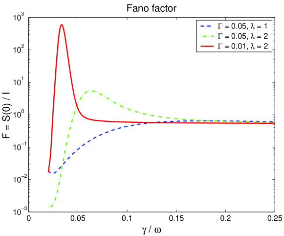
Figure 5.8: Fano factor for the SDQS vs. damping $\gamma$. The mechanical dissipation rate $\gamma$ and the electrical rate $\Gamma=\Gamma_{L}=\Gamma_{R}$ are given in units of the mechanical frequency $\omega$. The tunneling length $\lambda$ in terms of $x_{0}=\sqrt{\hbar/(m\omega)}$. The other parameters are $d=0.5x_{0}$ and $T=0$. The very low noise in the shuttling (low damping) regime is a sign of ordered transport. The huge super-poissonian Fano factors corresponds to the onset of the coexistence regime.

A comparison with the current curves (fig. 5.5) shows that the peak in the Fano factor corresponds to the transition region from the tunneling to the shuttling current. Similarly the correspondence can be established also with the Wigner function distribution: the region of damping in which tunneling (dot in $W_{\rm tot}$) and shuttling (ring in $W_{\rm tot}$) features coexist is associated with a super-poissonian Fano factor. The very low ($F\approx 0.01$) Fano factors for low damping are a signature of the deterministic transport that takes place in the shuttling regime. It is interesting to note that this regularity persists also deep in the quantum regime as can be seen for $\Gamma=0.05\omega$ and $\lambda=x_{0}$. The relative uncertainty in the amplitude of the oscillation (see Fig. 5.1) does not seem to influence the current noise.

Chapter 6 The three regimes

The shuttle devices are characterized by a strong interplay between electrical and mechanical degrees of freedom, the electrostatic force modifying the mechanical dynamics of the oscillating dot and the position dependent tunneling amplitudes representing the back-action of the mechanical degree of freedom on the electrical dynamics. Despite the complexity expected because of the non-linear couplings, the dynamics of shuttle devices (at least in the SDQS realization) can be classified into three operating regimes defined by different relations between the typical time scales in the device. We make in the next sections a qualitative analysis of these regimes leaving to the next chapter the definition of the simplified models and the quantitative comparison between full and approximate description in terms of the investigation tools that we introduced in the previous chapter.

6.1 Tunneling

The tunneling regime is the high damping regime in which the relaxation time of the mechanical oscillation (inverse of the damping rate $\gamma$) is much shorter than the typical electronic time (inverse of the average tunneling rate $\bar{\Gamma}$). We also assume that the oscillator dynamics is under-damped:

$$\omega\gg\gamma\gg\bar{\Gamma}={\rm Tr}_{\rm sys}\left\{\Gamma_{R}(x)|1\rangle\!\langle 1|\sigma^{\rm stat}\right\}$$ (6.1)

The dynamics of the device can be described by a four steps cycle (see Fig. 6.1):

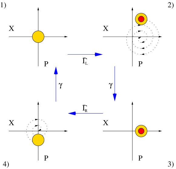
Figure 6.1: Schematic picture of the tunneling regime. In the scheme we represent the motion of quantum dot in the phase space of the oscillator (position $X$ and momentum $P$) and at the same time we keep track of the charge degree of freedom. The four steps on the cycle are described in detail in the text.

1. The dot is empty and in its mechanical ground state. We represent it in the phase space at rest in the origin and neglect in this simplified description the quantum indetermination and/or thermal noise that would blur the mechanical phase space distribution.

2. A tunneling event (from the source lead) and consequent electrostatic force $e\mathcal{E}$ perturbs the mechanical state of the dot which gets a positive position and momentum and starts to oscillate due to the harmonic restoring forces. The amplitude of the dot oscillations diminishes due to the dissipative environment. The $1)\to 2)$ transition takes place randomly but with a defined rate $\bar{\Gamma}_{L}$: the average injection rate.

3. The dot is at rest in the charged state equilibrium position ($d=\frac{e\mathcal{E}}{m\omega^{2}}$) given by the combination of the harmonic potential and the electrostatic force. The transition $2)\to 3)$ takes place in the short relaxation time $1/\gamma$.

4. A second tunnelling event (now towards the drain lead) brings back the dot into the original harmonic potential. The empty dot (distribution function) spirals towards the origin of the phase space and the cycle is closed. The time scale of the $3)\to 4)$ transition is given by the inverse ejection rate $1/\bar{\Gamma}_{R}$ while the mechanical relaxation $4)\to 1)$ takes place within a time $1/\gamma$.

Since the mechanical damping rate is much larger than the average injection (ejection) rate the system will stay most of the time in the configuration 1 and 3. A description with a coarse grained time do not see the mechanical transients 2 and 3 and is given in terms of a two state model: empty dot in the origin and charged dot in the shifted equilibrium position.

6.2 Shuttling

The shuttling regime is characterized by a non-adiabatic interplay between electrical and mechanical degrees of freedom of the device. In particular the average injection and ejection rate exactly matches the mechanical frequency of the oscillator. The mechanical relaxation rate is much smaller than the mechanical frequency:

$$\gamma\ll\frac{\omega}{2\pi}=\bar{\Gamma}$$ (6.2)

In the shuttling regime the quantum dot oscillates in a self-sustained stable limit cycle: all the energy pumped per cycle into the system by the electrostatic force is dissipated in the environment during the oscillation itself. Also the shuttling regime can be described by a four step cycle (see Fig. 6.2):

1. The quantum dot, close to the source lead, is charged with an extra electron. The Coulomb blockade prevents any other charging event. The high chemical potential on the left lead makes the charging incoherent and irreversible.

2. Under the combined effect of the mechanical restoring force and the electrostatic force the dot is accelerated towards the right lead. The tunneling parameters have been chosen such that the dot is effectively decoupled from the left and right lead while close to the center of the oscillation. Thus the electrical state of the device remains unchanged along most of the oscillation trajectory.

3. The dot is close to the right lead and the very high ejection rate makes the electron unloading practically deterministic.

4. The empty dot returns towards the left lead under the action of the restoring force of the harmonic oscillator and completes the cycle.

This sequential “classical” description of the shuttling regime is motivated by the phase space analysis of the previous chapter. The current saturation of one electron per cycle and the low noise seem to confirm this interpretation. At least for the most classical parameters range we will see that the dynamics is well described by a “trajectory” in the phase space of the system where a mean field charge coordinate has been added to the mechanical position and momentum.

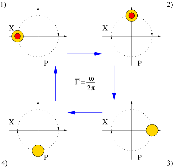
Figure 6.2: Schematic picture of the shuttling regime.

6.3 Coexistence

At intermediate damping rates the shuttle device shows bistability. Under these conditions neither the tunneling or the shuttling are globally stable regimes and the noise present in the system (shot noise of the charge transfer, thermal noise, quantum mechanical indetermination) causes the random switching between the two processes. The bistability is represented in the stationary distribution function by the coexisting tunneling and shuttling features. We showed that tunneling and shuttling regimes are associated with different average currents. It is not difficult to imagine that the current of the coexistence regime is an average of the shuttling and tunneling currents weighted on the probability for the device to be in one or in the other regime. The slow switching between these two currents generates the peculiar huge super-poissonian Fano factor that also characterized the coexistence regime. It is possible to demonstrate that the zero frequency current noise associated to a slow dichotomous switching between two states with average currents $I_{+}$ and $I_{-}$ reads:

$$S(0)=\frac{\alpha\beta}{(\alpha+\beta)^{3}}(I_{+}-I_{-})^{2}$$ (6.3)

where $\alpha$ ($\beta$) is the switching rate from state 1 to 2 (2 to 1). It is important that the average transition time between shuttling and tunneling is the longest time scale in the system dynamics. This fact ensures:

1. Many tunneling or shuttling events before the regime transition take place and thus there exists a well defined average current for the two “states”;

2. A huge Fano factor $F\approx I_{sh}/\alpha$.

The time resolved dynamics for the coexistence regime is depicted in figure 6.3 where the transition rates between the two regime are represented respectively by $\Gamma_{out}$ (tunneling $\to$ shuttling) and $\Gamma_{in}$ (shuttling $\to$ tunneling). The names ($in$ and $out$) associated to the transition rates are motivated by the dynamics of the mechanical amplitude during the transition. The average oscillation amplitude are very different in the shuttling and tunneling regime and can be used to identify the two states. In fact we will describe the switching dynamics in terms of a bistable potential with the amplitude as the effective coordinate.

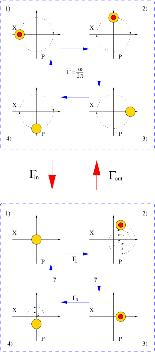
Figure 6.3: Schematic picture of the coexistence regime.

Chapter 7 Simplified models

We qualitatively described in the previous chapter three possible operating regimes for shuttle-devices. They represent for the SDQS the whole scenario of possible dynamics. Part of the complexity of the TDQS is also captured in this scheme. The specific separation of time scales allows us to identify the relevant variables and describe each regime by a specific simplified model. Models for the tunneling, shuttling and coexistence regime are analyzed separately in the three following sections. We also give a comparison with the full description in terms of Wigner distributions, current and current-noise to prove that the models, at least in the limits set by the chosen investigation tools, capture the relevant dynamics.

7.1 Renormalized resonant tunneling

The electrical dynamics is definitely the slowest in the tunneling regime since the mechanical relaxation time (much longer in itself than the oscillation period) is much shorter than the average injection or ejection time. We already noticed (sec. 6.1) that, because of this time-scale separation, the observation of the device dynamics would most of the time show two mechanically frozen states:

0.

Empty dot at rest in the oscillator equilibrium position

1.

Charged dot in the shifted equilibrium position of the harmonic oscillator perturbed by the constant electrostatic force $e\mathcal{E}$.

We combine this observation with a quantum description of the mechanical oscillator and possible thermal noise under the assumption that the $n$-resolved reduced density matrix of the device can be written in the form:

$$\begin{split}\sigma_{00}^{(n)}(t)&=p^{(n)}_{00}(t)\sigma_{\rm th}(0)\\ \sigma_{11}^{(n)}(t)&=p^{(n)}_{11}(t)\sigma_{\rm th}(e\mathcal{E})\end{split}$$ (7.1)

where

$$\sigma_{\rm th}(\mathcal{F})=\frac{e^{-\beta(H_{\rm osc}-\mathcal{F}x)}}{{\rm Tr}_{\rm osc}\left[e^{-\beta(H_{\rm osc}-\mathcal{F}x)}\right]}$$ (7.2)

is the thermal density matrix of a harmonic oscillator subject to an external force $\mathcal{F}$. The functions $p^{(n)}_{00}(t)$ and $p^{(n)}_{11}(t)$ represent the probability to find the system respectively in the state 0 or 1 that we described above when $n$ electrons have tunnelled through the dot. The sum over all possible device and bath configurations is $\sum_{n}p^{(n)}_{00}(t)+p^{(n)}_{11}(t)=1$ at all times. The equations of motion for the probabilities $p^{(n)}_{ii}(t)$ can be derived by inserting the assumption (7.1) in the $n$-GME (3.98) and taking the trace over the mechanical degrees of freedom:

$$\begin{split}\dot{p}^{(n)}_{00}&=\tilde{\Gamma}_{R}\,p^{(n-1)}_{11}-\tilde{\Gamma}_{L}\,p^{(n)}_{00}\\ \dot{p}^{(n)}_{11}&=\tilde{\Gamma}_{L}\,p^{(n)}_{00}-\tilde{\Gamma}_{R}\,p^{(n)}_{11}\end{split}$$ (7.3)

where

$$\begin{split}\tilde{\Gamma}_{L}&={\rm Tr}_{\rm osc}\left[\Gamma_{L}e^{-\frac{2x}{\lambda}}\sigma_{\rm th}(0)\right]\\ \tilde{\Gamma}_{R}&={\rm Tr}_{\rm osc}\left[\Gamma_{R}e^{\frac{2x}{\lambda}}\sigma_{\rm th}(e\mathcal{E})\right]\end{split}$$ (7.4)

are the injection and ejection rates renormalized to take into account the quantum/thermal distribution of the harmonic oscillator position. The master equation (7.3) summed over the number $n$ of electrons collected in the right lead reads:

$$\begin{split}\dot{p}_{00}&=\tilde{\Gamma}_{R}\,p_{11}-\tilde{\Gamma}_{L}\,p_{00}\\ \dot{p}_{11}&=\tilde{\Gamma}_{L}\,p_{00}-\tilde{\Gamma}_{R}\,p_{11}\end{split}$$ (7.5)

where we have introduced the occupation probabilities of the state $i$ $p_{ii}\equiv\sum_{n=0}^{\infty}p_{ii}^{(n)}$. Equations (7.5) describe the dynamics of a resonant tunneling device. The effects of the movable grain are contained in the effective rates $\tilde{\Gamma}_{L},\tilde{\Gamma}_{R}$.

7.1.1 Electrical rates

The renormalized electrical rates can be calculated analytically as functions of the model parameters. The calculation gives the exact contribution of the quantum mechanical and thermal noise to the electrical dynamics. We first consider the limit of very low temperatures $k_{B}T\ll\hbar\omega$. Only the ground state of the harmonic oscillator is occupied and the renormalized injection rate reads:

$$\begin{split}\tilde{\Gamma}_{L}&={\rm Tr}_{\rm osc}\left[|0\rangle\!\langle 0|\Gamma_{L}e^{-2x/\lambda}\right]=\Gamma_{L}\langle 0|e^{-\frac{2x}{\lambda}}|0\rangle\\ &=\frac{\Gamma_{L}}{\sqrt{\pi}}\int_{-\infty}^{+\infty}d\xi\,\exp\left[-\left(\xi^{2}+\frac{2\xi x_{0}}{\lambda}\right)\right]=\Gamma_{L}e^{(\frac{x_{0}}{\lambda})^{2}}\end{split}$$ (7.6)

where $|0\rangle$ is the vector representing the ground state of the harmonic oscillator and $x_{0}=\sqrt{\hbar/(m\omega)}$. For the calculation of the renormalized ejection rate it is useful to introduce the displacement unitary operator:

$$D(l)=e^{-\frac{i}{\hbar}lp}$$ (7.7)

with the properties:

$$\begin{split}D(l)dD^{{\dagger}}(l)&=d-l\sqrt{{\textstyle\frac{m\omega}{2\hbar}}}\\ D(l)d^{{\dagger}}D^{{\dagger}}(l)&=d^{{\dagger}}-l\sqrt{{\textstyle\frac{m\omega}{2\hbar}}}\\ D(l)xD^{{\dagger}}(l)&=x-l\end{split}$$ (7.8)

where $x,p$ are the position and momentum operators and $d^{{\dagger}},d$ are the creation and annihilation operators for the harmonic oscillator. In terms of the displacement operator $D$ the density matrix $\sigma_{\rm th}(\mathcal{F})$ can be written:

$$\sigma_{\rm th}(\mathcal{F})=D\left({\textstyle\frac{\mathcal{F}}{m\omega^{2}}}\right)\sigma_{\rm th}(0)D^{{\dagger}}\left({\textstyle\frac{\mathcal{F}}{m\omega^{2}}}\right)$$ (7.9)

Only the displaced ground state contributes to the renormalized ejection rate:

$$\begin{split}\tilde{\Gamma}_{R}&={\rm Tr}_{\rm osc}\left[D(d)|0\rangle\!\langle 0|D^{{\dagger}}(d)\,\Gamma_{R}e^{-2x/\lambda}\right]\\ &=\Gamma_{R}\langle 0|D^{{\dagger}}(d)\,e^{\frac{2x}{\lambda}}\,D(d)|0\rangle\\ &=\Gamma_{R}e^{\frac{2d}{\lambda}}\langle 0|e^{\frac{2x}{\lambda}}|0\rangle=\Gamma_{R}e^{\frac{2d}{\lambda}+\left(\frac{x_{0}}{\lambda}\right)^{2}}\end{split}$$ (7.10)

where $d=\frac{e\mathcal{E}}{m\omega^{2}}$.

As expected the ejection rate is modified by the “classical” shift $d$ of the equilibrium position due to the electrostatic force on the charged dot. Somehow unexpectedly both rates are also enhanced by the quantum uncertainty in the position present in the oscillator ground state. The relevance of the quantum correction is given by the ratio between the zero point position dispersion $x_{0}$ and the tunneling length $\lambda$: the smaller the ratio the smaller the correction.

The calculation of the finite temperature rates is problematic due to the presence in the trace of the product of the exponentials of two non commutative operators ($H_{\rm osc},x$). We solve the problem using the low temperature calculation just performed and some symmetry arguments. First we notice that the density matrix $\sigma_{\rm th}$ is the stationary solution of the GME:

$$\dot{\sigma}=-\frac{i}{\hbar}[H_{\rm osc},\sigma]-\frac{i\gamma}{2\hbar}[x,\{p,\sigma\}]-\frac{\gamma m\omega}{\hbar}\left[n_{B}(\omega)+\frac{1}{2}\right][x,[x,\sigma]]$$ (7.11)

We express the trace in the position (generalized) basis $|q\rangle$ and the renormalized rates take the form:

$$\begin{split}\tilde{\Gamma}_{L}&=\Gamma_{L}\int dq\,P_{\rm th}(q)e^{-\frac{2q}{\lambda}}\\ \tilde{\Gamma}_{R}&=\Gamma_{R}e^{\frac{2d}{\lambda}}\int dq\,P_{\rm th}(q)e^{\frac{2q}{\lambda}}\end{split}$$ (7.12)

where we have introduced the coordinate probability distribution $P_{\rm th}(q)\equiv\langle q|\sigma_{\rm th}|q\rangle$. We encountered this distribution already in section (4.1) in the axiomatical definition of the Wigner function. We required specifically:

$$\int dpW(q,p,t)=\langle q|\sigma|q\rangle$$ (7.13)

The problem is thus shifted to the calculation of the Wigner function associated with the thermal density matrix $\sigma_{\rm th}$. The dynamics of the Wigner distribution is given by the Fokker-Planck equation related to the GME (7.11):

$$\frac{\partial W}{\partial\tau}=\left[X\frac{\partial}{\partial P}-P\frac{\partial}{\partial X}+\frac{\gamma}{\omega}\frac{\partial}{\partial P}\left(P+\frac{\partial}{\partial P}\right)\right]\,W$$ (7.14)

where we have defined the adimensional variables:

$$\tau=\omega t,\quad X=\frac{q}{\ell},\quad P=\frac{p}{m\omega\ell}$$ (7.15)

and $\ell=\sqrt{\frac{\hbar}{2m\omega}(2n_{B}+1)}$. The Fokker-Planck equation (7.14) does not depend on the temperature. The stationary solution is the Gaussian in $X$ and $P$

$$W^{\rm stat}(X,P)=\frac{1}{2\pi}\exp\left(-\frac{X^{2}+P^{2}}{2}\right)$$ (7.16)

with no parameters. The position distribution function $P_{\rm th}(q)$ thus depends on the temperature only in the scaling factor and has the same functional form (Gaussian) of the zero temperature case:

$$P_{\rm th}(q)=\frac{1}{\sqrt{2\pi\ell^{2}}}\exp\left(-\frac{q^{2}}{2\ell^{2}}\right)$$ (7.17)

Finally we insert (7.17) into (7.12) and perform the gaussian integrals to obtain the finite temperature rates:

$$\begin{split}\tilde{\Gamma}_{L}&=\Gamma_{L}e^{2\left(\frac{\ell}{\lambda}\right)^{2}}\\ \tilde{\Gamma}_{R}&=\Gamma_{R}e^{\frac{2d}{\lambda}+2\left(\frac{\ell}{\lambda}\right)^{2}}\end{split}$$ (7.18)

In the low temperature limit equations (7.18) obviously reduce to (7.6) and (7.10). The high temperature limit $k_{B}T\gg\hbar\omega$ is also interesting:

$$\begin{split}\tilde{\Gamma}_{L}&=\Gamma_{L}e^{2\left(\frac{\lambda_{\rm th}}{\lambda}\right)^{2}}\\ \tilde{\Gamma}_{R}&=\Gamma_{R}e^{\frac{2d}{\lambda}+2\left(\frac{\lambda_{\rm th}}{\lambda}\right)^{2}}\end{split}$$ (7.19)

In this case the renormalization is the more effective the larger is the thermal length $\lambda_{\rm th}=\sqrt{k_{B}T/(m\omega^{2})}$ compared to the tunneling length $\lambda$.

7.1.2 Phase-space distribution

The phase space distribution for the stationary state of the simplified model for the tunneling regime is built on the Wigner representation of the thermal density matrix $\sigma_{\rm th}$ and the stationary solution of the system (7.5) for the occupation $p_{ii}$ of the electromechanical states $i$. The latter is easily expressed in terms of the renormalized rates $\tilde{\Gamma}_{L,R}$:

$$\begin{split}p_{00}^{\rm stat}&=\frac{\tilde{\Gamma}_{R}}{\tilde{\Gamma}_{L}+\tilde{\Gamma}_{R}}\\ p_{11}^{\rm stat}&=\frac{\tilde{\Gamma}_{L}}{\tilde{\Gamma}_{L}+\tilde{\Gamma}_{R}}\end{split}$$ (7.20)

We have already met the Wigner distribution corresponding to the thermal density matrix $\sigma_{\rm th}$ in Eq. (7.16). We now rewrite it in terms of the canonical variables $(q,p)$:

$$\sigma_{\rm th}(0)\to W_{\rm th}(q,p)=\frac{1}{2\pi m\omega\ell^{2}}\exp\left\{-\frac{1}{2}\left[\left(\frac{q}{\ell}\right)^{2}+\left(\frac{p}{\ell m\omega}\right)^{2}\right]\right\}$$ (7.21)

The calculation of the Wigner function for the displaced thermal distribution $\sigma_{\rm th}(e\mathcal{E})$ can be performed using the properties of the displacement operators $D$:

$$\begin{split}\sigma_{\rm th}(e\mathcal{E})&\to\frac{1}{2\pi\hbar}\int d\xi\left\langle q-\frac{\xi}{2}\right|D(d)\sigma_{\rm th}(0)D^{{\dagger}}(d)\left|q+\frac{\xi}{2}\right\rangle\exp\left(\frac{i}{\hbar}p\xi\right)\\ &=\frac{1}{2\pi\hbar}\int d\xi\left\langle q-d-\frac{\xi}{2}\right|\sigma_{\rm th}(0)\left|q-d+\frac{\xi}{2}\right\rangle\exp\left(\frac{i}{\hbar}p\xi\right)\\ &=W_{\rm th}(q-d,p)\end{split}$$ (7.22)

where we have used the property $D(l)|a\rangle=|a-l\rangle$ that we can be proven as follows: given $|a\rangle$ eigenvector for the position operator $x$ with eigenvalue $a$

$$\begin{split}xD(l)|a\rangle&=D(l)\,D^{{\dagger}}(l)\,x\,D(l)|a\rangle\\ &=D(l)(x-l)|a\rangle=(a-l)D(l)|a\rangle\end{split}$$ (7.23)

The stationary solution of the Klein-Kramers equation (4.32) in the tunneling regime limit thus reads:

$$\begin{split}W_{00}^{\rm stat}(q,p)&=\frac{\tilde{\Gamma}_{R}}{\tilde{\Gamma}_{L}+\tilde{\Gamma}_{R}}W_{\rm th}(q,p)\\ W_{11}^{\rm stat}(q,p)&=\frac{\tilde{\Gamma}_{L}}{\tilde{\Gamma}_{L}+\tilde{\Gamma}_{R}}W_{\rm th}(q-d,p)\end{split}$$ (7.24)

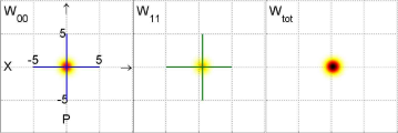
Figure 7.1: Wigner distribution functions for the SDQS in the tunneling regime. calculated numerically using the full description. Coordinates (horizontal axis) are measured in terms of $x_{0}$, momenta (vertical axis) in terms of $m\omega x_{0}$. The crosses indicates the cuts in the phase space along which we perform the comparison between numerical and analytical solution shown in figure 7.2. The parameters are: $\Gamma_{L}=\Gamma_{R}=0.01\omega$, $\gamma=0.25\omega$, $d=0.5x_{0}$, $\lambda=2x_{0}$, $T=0$.

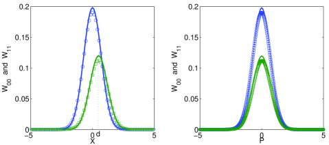
Figure 7.2: Comparison between the numerical and the analytical results for the Wigner distribution functions. The squares (circles) are numerical results for the parameters mentioned in figure 7.1 in the charged (empty) dot configuration, and the full lines represent the analytical calculations. We also plotted with dots the numerical results for $\Gamma=0.001\omega$.

The stationary distribution of the tunneling model is completely determined by the length $\ell$ and associated momentum $m\omega\ell$, the equilibrium position shift $d$ and the tunneling length $\lambda$. The electronic and mechanical relaxation rates $\gamma$ and $\Gamma_{L,R}$ drop out from the solution and only set the range of applicability of the simplified model.

In figures 7.1, 7.2 and 7.3 we compare the Wigner functions calculated both analytically and numerically in the tunneling regime. They show in general a very good agreement. In particular we notice in Fig. 7.2 that the convergence to the tunneling regime is not yet complete for $\gamma=0.25\omega$ and $\Gamma_{L,R}=0.01\omega$. To check the theory we diminished the bare electrical rate further (the quantum corrections are negligible since $\lambda=2x_{0}$, the classical shift can be taken into account and gives a factor $e\approx 2.7$ which does not change the analysis) and kept the mechanical damping fixed to “maintain” the condition $\gamma\ll\omega$. For $\Gamma=0.001\omega$ we got perfect agreement. We also analyze the temperature dependence of the stationary Wigner function distribution (Fig. 7.3) and verify the scaling given by the temperature dependent length $\ell$.

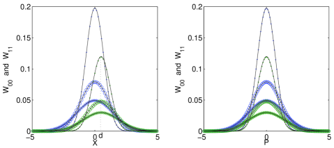
Figure 7.3: Tunneling Wigner distributions as a function of the temperature. The relevant parameters are: $\gamma=0.25\omega$, $\Gamma=0.001\omega$, $n_{B}=0,0.75,1.5$ respectively represented by dots, circles and asterisks. Full lines are the analytical results. See Fig: 7.1 for the other parameters and the scales.

7.1.3 Current

The current through the SDQS towards the right lead is given by the general formula:

$$I_{R}(t)=\sum_{n=0}^{\infty}n\dot{P}_{n}(t)$$ (7.25)

In the tunneling limit the probabilities $P_{n}(t)$ are be expressed in terms of $p^{(n)}_{ii}(t)$ since:

$$P_{n}(t)={\rm Tr}_{\rm osc}[p^{(n)}_{00}(t)\sigma_{\rm th}(0)+p^{(n)}_{11}(t)\sigma_{\rm th}(e\mathcal{E})]=p_{00}^{(n)}(t)+p_{11}^{(n)}(t)$$ (7.26)

Apart from the renormalized electronic rates the system has no sign of the oscillator degree of freedom and can be treated formally as a static quantum dot. We write in complete analogy with (3.54) the right (left) lead time dependent current:

$$\begin{split}I_{R}(t)&=\tilde{\Gamma}_{R}p_{11}(t)\\ I_{L}(t)&=\tilde{\Gamma}_{L}p_{00}(t)\end{split}$$ (7.27)

In the stationary limit they coincide:

$$I^{\rm stat}=\begin{array}[]{c}\nearrow\\ \searrow\end{array}\begin{array}[]{c}\lim_{t\to\infty}I_{R}(t)=\tilde{\Gamma}_{R}p^{\rm stat}_{11}=\bar{\Gamma}_{R}\\ \\ \\ \lim_{t\to\infty}I_{L}(t)=\tilde{\Gamma}_{L}p^{\rm stat}_{00}=\bar{\Gamma}_{L}\end{array}\begin{array}[]{c}\searrow\\ \nearrow\end{array}=\frac{\tilde{\Gamma}_{R}\tilde{\Gamma}_{L}}{\tilde{\Gamma}_{L}+\tilde{\Gamma}_{R}}=\bar{\Gamma}$$ (7.28)

We stress the difference between $\bar{\Gamma}_{L(R)}$ and $\tilde{\Gamma}_{L(R)}$: while the first is the average injection (ejection rate) and thus represents the current through the device, the second is an average over the mechanical distribution function of the position dependent rate operator. Despite being an average rate it does not take into account the charge state of the dot (and the Coulomb blockade) and thus cannot represent the current through the device. We show in figure 7.4 the current calculated numerically and the asymptotic value of the tunneling regime given by Eq. (7.28).

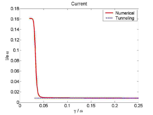
Figure 7.4: Current as a function of the damping for the SDQS. The asymptotic tunneling limit is indicated. The parameters are: $\Gamma_{L}=\Gamma_{R}=0.01\omega$, $\gamma=0.25\omega$, $d=0.5x_{0}$, $\lambda=2x_{0}$, $T=0$.

7.1.4 Current-noise

The calculation of the current noise and Fano factor in the tunneling regime is interesting since it gives us the opportunity to explain the concepts and methods we introduced in section 5.3 still keeping a computational level analytically affordable due to the much lesser number of degrees of freedom of the effective model.

We start with the MacDonald formula for the zero frequency current noise:

$$S(0)=\lim_{t\to+\infty}\frac{d}{dt}\Big{[}\sum_{n=0}^{\infty}n^{2}P_{n}(t)-\big{(}\sum_{n=0}^{\infty}nP_{n}(t)\big{)}^{2}\Big{]}$$ (7.29)

where $P_{n}(t)=p_{00}^{(n)}+p_{11}^{(n)}$ and the equation of motion for $p_{ii}^{(n)}$ are:

$$\begin{split}\dot{p}^{(n)}_{00}&=\tilde{\Gamma}_{R}\,p^{(n-1)}_{11}-\tilde{\Gamma}_{L}\,p^{(n)}_{00}\\ \dot{p}^{(n)}_{11}&=\tilde{\Gamma}_{L}\,p^{(n)}_{00}-\tilde{\Gamma}_{R}\,p^{(n)}_{11}\end{split}$$ (7.30)

We identify the effective Liouvillean $\mathcal{L}$ for the relevant variables $p_{ii}(t)$ in the model:

$$\mathcal{L}=\begin{pmatrix}-\tilde{\Gamma}_{L}&\tilde{\Gamma}_{R}\\ \tilde{\Gamma}_{L}&-\tilde{\Gamma}_{R}\end{pmatrix}$$ (7.31)

The evaluation of the different terms of the current-noise can be carried out by introducing the generating functions $F_{ii}(t;z)=\sum_{n}p_{ii}^{(n)}(t)z^{n}$ and following the same reasoning we indicated in section 5.3.2. The result is formally the same: we express the Fano factor in terms of the stationary probabilities $p_{ii}^{\rm stat}$ and the pseudoinverse of the the Liouvillean $\mathcal{QL}^{-1}\mathcal{Q}$.

$$F=1-\frac{2}{I^{\rm stat}}\left\|\begin{pmatrix}0&\tilde{\Gamma}_{R}\\ 0&0\end{pmatrix}\mathcal{QL}^{-1}\mathcal{Q}\begin{pmatrix}0&\tilde{\Gamma}_{R}\\ 0&0\end{pmatrix}\begin{pmatrix}p_{00}^{\rm stat}\\ p_{11}^{\rm stat}\end{pmatrix}\right\|_{1}$$ (7.32)

where $\|\bullet\|_{1}$ is the sum of the elements of the vector. The projectors $\mathcal{P}$ and $\mathcal{Q}$, built from their definition (see sec. 5.3.2), have the matrix form:

$$\mathcal{P}=\begin{pmatrix}p_{00}^{\rm stat}&p_{00}^{\rm stat}\\ p_{11}^{\rm stat}&p_{11}^{\rm stat}\end{pmatrix},\quad\mathcal{Q}=\begin{pmatrix}\phantom{-}p_{11}^{\rm stat}&-p_{00}^{\rm stat}\\ -p_{11}^{\rm stat}&\phantom{-}p_{00}^{\rm stat}\end{pmatrix}.$$ (7.33)

For the explicit calculation of Eq. (7.32) we define the auxiliary vector $\Sigma$:

$$\Sigma=\begin{pmatrix}\Sigma_{00}\\ \Sigma_{11}\end{pmatrix}=\mathcal{QL}^{-1}\mathcal{Q}\begin{pmatrix}0&\tilde{\Gamma}_{R}\\ 0&0\end{pmatrix}\begin{pmatrix}p_{00}^{\rm stat}\\ p_{11}^{\rm stat}\end{pmatrix}$$ (7.34)

that satisfies the equation

$$\mathcal{L}\Sigma=\mathcal{Q}\begin{pmatrix}0&\tilde{\Gamma}_{R}\\ 0&0\end{pmatrix}\begin{pmatrix}p_{00}^{\rm stat}\\ p_{11}^{\rm stat}\end{pmatrix}=\tilde{\Gamma}_{R}(p_{11}^{\rm stat})^{2}\begin{pmatrix}1\\ -1\end{pmatrix}$$ (7.35)

Together with the condition $\Sigma_{00}+\Sigma_{11}=0$ we can calculate $\Sigma$ and by substitution into (7.32) find the Fano factor $F$:

$$F=1-\frac{2\tilde{\Gamma}_{R}\Sigma_{11}}{I^{\rm stat}}=1-\frac{2\tilde{\Gamma}_{R}(\tilde{\Gamma}_{L}+\tilde{\Gamma}_{R})}{\tilde{\Gamma}_{L}\tilde{\Gamma}_{R}}\frac{\tilde{\Gamma}_{R}\tilde{\Gamma}_{L}^{2}}{(\tilde{\Gamma}_{L}+\tilde{\Gamma}_{R})^{3}}=\frac{\tilde{\Gamma}_{L}^{2}+\tilde{\Gamma}_{R}^{2}}{(\tilde{\Gamma}_{L}+\tilde{\Gamma}_{R})^{2}}$$ (7.36)

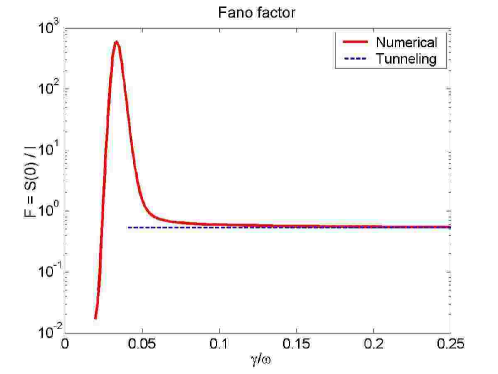
Figure 7.5: Current-noise as a function of the damping for the SDQS. The asymptotic tunneling limit is indicated. The parameters are: $\Gamma_{L}=\Gamma_{R}=0.01\omega$, $\gamma=0.25\omega$, $d=0.5x_{0}$, $\lambda=2x_{0}$, $T=0$.

7.2 Shuttling: a classical transport regime

The simplified model for the shuttling dynamics is based on the observation –extracted from the full description– that the system exhibits in this operating regime extremely low Fano factors ($F\approx 10^{-2}$). In the simplified model we assume that there is no noise at all in the system. Its state is represented by a point that moves on a trajectory in the 3-dimensional device phase-space of position, momentum and charge of the oscillating dot. It is hard not to imagine the charge on the oscillating dot as a stochastic variable governed by tunnelling processes. Nevertheless in the shuttling regime the tunneling events are made effectively deterministic since they are very highly probable at specific times settled by the mechanical dynamics. On the other hand, due to the electrostatic force $e\mathcal{E}$ acting on the charged dot that mirrors the electrical dynamics into a mechanical acceleration only “deterministic” tunneling events can produce a regular mechanical dynamics. We discuss in the next session the derivation of the equations of motion for this semiclassical model and then compare the results with the full quantum description.

7.2.1 Equation of motion for the relevant variables

The dynamics of the SDQS is described by the set of coupled Klein-Kramers equations (4.32). In order to implement the zero noise assumption we first set $T=0$ and simplify the equations further by neglecting all the terms of the $\hbar$ expansion since we assume the classical action of the oscillator to be much larger than the Planck constant. We obtain:

$$\begin{split}\frac{\partial W_{00}^{\rm cl}}{\partial\tau}=&\left[X\frac{\partial}{\partial P}-P\frac{\partial}{\partial X}+\frac{\gamma}{\omega}\frac{\partial}{\partial P}P\right]\,W_{00}^{\rm cl}\\ &-\frac{\Gamma_{L}}{\omega}e^{-2X}W_{00}^{\rm cl}+\frac{\Gamma_{R}}{\omega}e^{2X}W_{11}^{\rm cl}\\ \frac{\partial W_{11}^{\rm cl}}{\partial\tau}=&\left[\left(X-\frac{d}{\lambda}\right)\frac{\partial}{\partial P}-P\frac{\partial}{\partial X}+\frac{\gamma}{\omega}\frac{\partial}{\partial P}P\right]\,W_{11}^{\rm cl}\\ &-\frac{\Gamma_{R}}{\omega}e^{2X}W_{11}^{\rm cl}+\frac{\Gamma_{L}}{\omega}e^{-2X}W_{00}^{\rm cl}\end{split}$$ (7.37)

where we have introduced the adimensional variables:

$$\tau=\omega t,\quad X=\frac{q}{\lambda},\quad P=\frac{p}{m\omega\lambda}$$ (7.38)

The superscript “cl” indicates that we are dealing with the classical limit of the Wigner function justified by the complete elimination of the quantum “diffusive” terms from the Fokker-Planck equations and thus indefinitely sharp distribution functions are now allowed. We can at this point introduce a separation Ansatz:

$$\begin{split}W_{00}^{\rm cl}(X,P,\tau)=p_{00}(\tau)\delta(X-X^{\rm cl}(\tau))\delta(P-P^{\rm cl}(\tau))\\ W_{11}^{\rm cl}(X,P,\tau)=p_{11}(\tau)\delta(X-X^{\rm cl}(\tau))\delta(P-P^{\rm cl}(\tau))\end{split}$$ (7.39)

where the trace over the system phase-space sets $p_{00}+p_{11}=1$. The variables $X^{\rm cl}$ and $P^{\rm cl}$ represent the position and momentum of the (center of mass) of the oscillating dot; $p_{11(00)}$ is the probability for the quantum dot to be charged (empty).

By inserting the Ansatz (7.39) into equation (7.37) summing over the charge index $i$ and matching the coefficients of the different distribution functions on the left and right hand side we obtain:

$$\begin{split}\dot{X}^{\rm cl}&=P^{\rm cl}\\ \dot{P}^{\rm cl}&=-X^{\rm cl}+\frac{d}{\lambda}p_{11}-\frac{\gamma}{\omega}P^{\rm cl}\\ \end{split}$$ (7.40)

In order to close the system of differential equations we need the equations of motion for $p_{ii}$ provided by the integration over $X$ and $P$ of (7.37) with the separation Ansatz:

$$\begin{split}\dot{p}_{00}&=-\frac{\Gamma_{L}}{\omega}e^{-2X^{\rm cl}}p_{00}+\frac{\Gamma_{R}}{\omega}e^{2X^{\rm cl}}p_{11}\\ \dot{p}_{11}&=\frac{\Gamma_{L}}{\omega}e^{-2X^{\rm cl}}p_{00}-\frac{\Gamma_{R}}{\omega}e^{2X^{\rm cl}}p_{11}\end{split}$$ (7.41)

Unfortunately the system of equations (7.40) and (7.41) is not equivalent to (7.37): integration and summation have introduced spurious solutions. If we substitute the Ansatz (7.39) into the equations (7.37) and use the equations of motion (7.40) and (7.41) we obtain the condition:

$$p_{00}p_{11}=0$$ (7.42)

The only differentiable solution for this equation is $p_{00}=0$ or $p_{11}=0$ for all times and is not satisfying the equation of motion (7.41). Strictly speaking there are no solutions of (7.37) in the form suggested in the Ansatz.

Nevertheless we can imagine that the electrical switching time between the only allowed charged ($p_{11}=1;\,p_{00}=0$) and empty ($p_{00}=1;\,p_{11}=0$) states is much shorter than the shortest mechanical time (the oscillator period $T=2\pi/\omega$ ). A solution of the system of equations (7.40) and (7.41) with this time scale separation could “almost everywhere” satisfy the condition (7.42) and, inserted into (7.39) represent a solution for (7.37).

We rewrite the set of equations (7.40) and (7.41) as:

$$\begin{split}\dot{X}&=P\\ \dot{P}&=-X+d^{*}Q-\gamma^{*}P\\ \dot{Q}&=\Gamma_{L}^{*}e^{-2X}(1-Q)-\Gamma_{R}^{*}e^{2X}Q\end{split}$$ (7.43)

where we have dropped for simplicity the “cl” superscript from the mechanical variables, we have renamed $p_{11}\equiv Q$ and used the trace condition $p_{00}=1-p_{11}$. We have also defined the rescaled parameters:

$$d^{*}=d/\lambda,\quad\gamma^{*}=\gamma/\omega,\quad\Gamma_{L,R}^{*}=\Gamma_{L,R}/\omega$$ (7.44)

7.2.2 Stable limit cycles

The set of coupled non-linear differential equations (7.43) represents the starting point of the analysis of the simplified model for the shuttling regime. We calculate the numerical solution for different values of the parameters and different initial condition. For the parameter values that correspond in the full description to the shuttling regime, the system has a limit cycle solution with the desirable time scale separation we discussed in the previous section. We report in figure 7.6 the typical appearance of the limit cycle. In the first graph (a) we show the charge $Q(\tau)$ as a function of time. The charge value is jumping periodically from 0 to 1 and back with a period equal to the mechanical period. The transition itself is almost instantaneous. The limit cycle is a trajectory in the 3D phase-space of the device $(X,P,Q)$. In the graphs (b), (c) and (d) of figure 7.6 three different projections of the trajectory are reported. The $X,P$ projection shows the characteristic circular trajectory of harmonic oscillations. In the $X,Q$ ($P,Q$) projection the position(momentum)-charge correlation is visible. From the combination of the two projection we can argue that the trajectory in the $X,Q$ graph is drawn clockwise during the cycle. The oscillating dot gets charged on the left, it is then carrying the charge towards the right and finally it unloads the electron to the right lead before returning empty towards the left. The amplitude of the oscillation is several times the tunneling length. All the qualitative features of the shuttling regime are present.

The full description of the SDQS in the shuttling regime has a phase space visualization in terms of a ring shaped stationary total Wigner distribution function. We can interpret this fuzzy ring as the probability distribution obtained from many different noisy realizations of (quasi) limit cycles. The stationary solution for the Wigner distribution is the result of a diffusive dynamics on an effective “Mexican hat” potential that involves both amplitude and phase of the oscillations. In the noise-free semiclassical approximation we turn off the diffusive processes and the point-like state describes in the shuttling regime a single trajectory with a definite constant amplitude and periodic phase. We expect this trajectory to be the average of the noisy trajectories represented by the Wigner distribution. In the third column of figure 7.7 the total Wigner function corresponding to different parameter realization of the shuttling regime is presented. The white circle is the semiclassical trajectory. In the first two columns the asymmetric sharing of the ring between the charged and empty states is also compared with the corresponding $Q=1$ and $Q=0$ portions of the semiclassical trajectory.

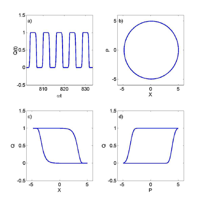
Figure 7.6: Different representations of the limit cycle solution of the system of differential equations (7.43) that describes the shuttling regime. a) Charge on the dot as a function of time. The charging and discharging times are the shortest time scales. b) Circular trajectory in the mechanical phase space: the motion of the dot is harmonic. c) Projection of the limit cycle in the charge position plane: the trajectory shows charge-position correlation. d) Projection of the limit cycle in the charge momentum plane: the trajectory shows charge-momentum correlation. $X$ is the coordinate in units of the tunneling length $\lambda$, while $P$ is the momentum in units of $m\omega\lambda$.

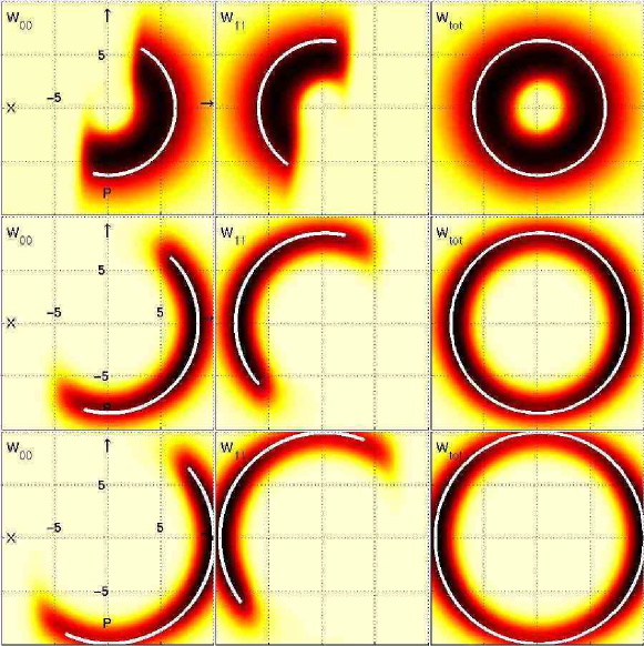
Figure 7.7: Correspondence between the Wigner function representation and the simplified trajectory limit for the shuttling regime. The white ring is the ($X,P$) projection of the limit cycle. The $Q=1$ and $Q=0$ portions of the trajectory are visible in the charged and empty dot graphs respectively. The parameters are $\gamma=0.02\omega$, $d=0.5x_{0}$, $\Gamma=0.05\omega$ in the first two rows and $\Gamma=0.01$ in the last one. The tunneling length is $\lambda=x_{0}$ in the first row and $\lambda=2x_{0}$ in the second and the third.

In the semiclassical description we also have direct access to the current as a function of the time. For example the right lead current reads:

$$I_{R}(\tau)=Q(\tau)\Gamma_{R}e^{2X(\tau)}$$ (7.45)

In figure 7.8 the right current is presented as a function of time for a few mechanical oscillation periods. The current is given by a series of spikes that well represent the single electron released to the right lead after being shuttled by the oscillating dot.

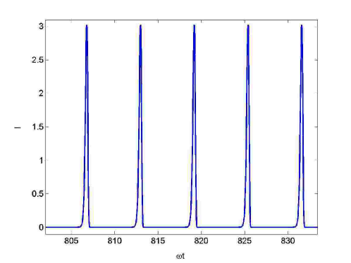
Figure 7.8: Time resolved shuttling current calculated on the limit cycle solution of the system of differential equations (7.43). The regular spikes well represent the single electron shuttled per cycle in this regime.

The average current is a coarse grained measurement of the time dependent current. Since the current is periodic, if the measurement time is long enough we obtain a stationary current:

$$I^{\rm stat}=\frac{1}{2\pi}\int_{\tau}^{\tau+2\pi}\!\!d\tau^{\prime}\,I_{R}(\tau^{\prime})$$ (7.46)

Since the current is a periodic function of time the average over one period is equal to the average over an infinite time. The numerical integration of the function plotted in figure 7.8 gives

$$I^{\rm stat}=0.15916$$ (7.47)

which is with impressive accuracy the “magic value” of $1/2\pi$ (i.e. one electron transferred per oscillation period).

Also for the TDQS we tried a semiclassical analysis of the shuttling regime. For the derivation of the semiclassical equations we start again from the Hamiltonian (2.9) but we consider $x$ and $p$ as classical variables. The GME equation for the reduced density matrix $\sigma$ is derived by keeping $x$ as a parameter ($p$ does not enter explicitly the formulation of the GME). Since the oscillator is treated classically also the elements of the density matrix $\sigma_{ij}$ are now real numbers and the trace sum rule can be used to reduce the effective number of equation for the electrical dynamics from 10 to 9. The GME in matrix notation reads:

$$\dot{\sigma}=-\frac{i}{\hbar}[H_{sys},\sigma]+\Xi[\sigma]$$ (7.48)

where

$$H_{\rm sys}=\frac{1}{2}m\omega^{2}x^{2}+\frac{p^{2}}{2m}+\begin{pmatrix}\frac{\Delta V}{2}&t_{L}(x)&0\\ t_{L}(x)&-\frac{\Delta V}{2x_{0}}x&t_{R}(x)\\ 0&t_{R}(x)&-\frac{\Delta V}{2}\end{pmatrix}$$ (7.49)

and the driving Liouvillean $\Xi$ has the form

$$\Xi[\sigma]=\Gamma\begin{pmatrix}1-\sigma_{LL}-\sigma_{CC}-\sigma_{RR}&0&-\sigma_{LR}/2\\ 0&0&-\sigma_{CR}/2\\ -\sigma_{RL}/2&-\sigma_{RC}/2&-\sigma_{RR}\end{pmatrix}$$ (7.50)

where we have taken $\Gamma_{L}=\Gamma_{R}=\Gamma$. As equation of motion for the mechanical variables $x$ and $p$ we take the Hamilton equations derived from the effective Hamiltonian

$$\langle H_{\rm sys}\rangle={\rm Tr}_{\rm el}[\sigma H_{\rm sys}]$$ (7.51)

where ${\rm Tr}_{\rm el}$ is the trace on the electronic states, combined with a phenomenological friction:

$$\begin{split}\dot{x}=&\frac{\partial\langle H_{\rm sys}\rangle}{\partial p}=\frac{p}{m}\\ \dot{p}=&-\frac{\partial\langle H_{\rm sys}\rangle}{\partial x}-\gamma p=-m\omega^{2}x+\frac{\Delta V}{2x_{0}}\sigma_{CC}-\gamma p\\ &+\frac{t_{L}}{\lambda}(\sigma_{CL}+\sigma_{LC})-\frac{t_{R}}{\lambda}(\sigma_{CR}+\sigma_{RC})\end{split}$$ (7.52)

The phase space has now 11 dimensions (9 electrical and 2 mechanical) but the principle is the same as in the SDQS. Also in this case the solution of the system of differential equations (7.48) and (7.52) exhibits for parameters that correspond to the shuttling regime a stable limit cycle solution. In figure 7.9 we compare the Wigner distribution function for the central dot with the projection on the $(x,p)$ plane of the limit cycle trajectory of the semiclassical approximation. The probability to find the electron on the central dot $\sigma_{CC}$ is not in general oscillating between 0 and 1. The red dots in the figure indicate the position of the maximum occupation. In the TDQS the half moon characteristic of the shuttling regime rotates in the phase space [10], close to the first two electromechanical resonances, as a function of the device bias. The correspondence between the darker areas of the Wigner function and the red dots in figure 7.9 shows that also this property is captured by the semiclassical approximation.

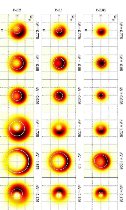
Figure 7.9: Comparison between the semiclassical approximation and the full description for TDQS. The figure shows the central dot Wigner function and the respective limit cycle. The dark dot on the trajectory is in correspondence with the maximum of the semiclassical occupation $\sigma_{CC}$. Also the phase space rotation is captured by the simplified model. The matching is best in the shuttling regime. See figure 5.4 for the details on the parameters.

7.3 Coexistence: a dichotomous process

The slowest dynamics in the coexistence regime is represented by the switching process between the shuttling and the tunneling regime. The amplitude of the dot oscillations is the relevant variable that is recording this slow dynamics. We analyze this particular operating regime of the SDQS in three steps. We first assume the slow switching mode between two different current channels and explore the consequences of this hypothesis in terms of current and current noise. We then derive the effective bistable potential for the amplitude associated with the slowest dynamics of the shuttle device in the coexistence regime. Finally we apply Kramers’ theory for escape rates to this effective potential and calculate the switching rates between the two amplitude equilibrium states corresponding to the local minima of the potential. We conclude the section comparing the (semi)analytical results of the simplified model with the numerical calculations corresponding to the full description.

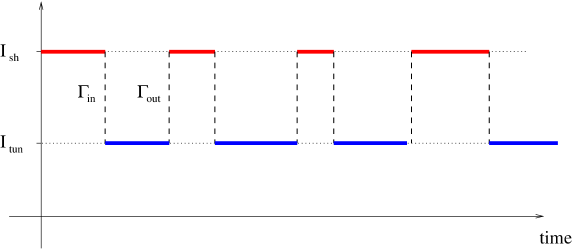
Figure 7.10: Schematic representation of the time evolution of the current in the dichotomous process between current modes. The scheme refers in particular to the SDQS coexistence regime where the currents involved are the shuttling ($I_{\rm sh}$) and the tunneling ($I_{\rm tun}$) currents and the names of switching rates $\Gamma_{\rm in}$ and $\Gamma_{\rm out}$ indicate the behaviour of the dot oscillation amplitude (the relevant variable in the model) during the transition.

7.3.1 Dichotomous process between current modes

Let us consider a bistable system with two different modes $+$ and $-$ and two different currents $I_{+}$ and $I_{-}$, respectively, associated with the modes. The system can switch between mode $+$ and $-$ randomly, but with definite rates: namely $\alpha$ for the process $+\to-$ and $\beta$ for the opposite $-\to+$. We collect this information in the master equation:

$$\dot{\mathbf{P}}=\frac{d}{dt}\begin{pmatrix}P_{+}\\ P_{-}\\ \end{pmatrix}=\begin{pmatrix}-\alpha&\phantom{-}\beta\\ \phantom{-}\alpha&-\beta\\ \end{pmatrix}\begin{pmatrix}P_{+}\\ P_{-}\\ \end{pmatrix}=\mathbf{LP}$$ (7.53)

where $P_{+}$ and $P_{-}$ are the probabilities to find the system in the mode “$+$” and “$-$” respectively.

The matrix notation suggests to read the equation (7.53) at a more general level and embed its classical rate dynamics into a quantum formalism.

Instead of the modes $+$ and $-$ we consider the state vectors $|+\rangle$ and $|-\rangle$: they define the Hilbert space of the quantum system. Density operators defined on this Hilbert space represent the state of the system. Since we are only interested in classical states we assume that the density matrix $\sigma$ is always diagonal in the $|+\rangle$, $|-\rangle$ basis. In terms of the probabilities $P$ the density matrix reads obviously:

$$\sigma=\begin{pmatrix}\sigma_{++}&\sigma_{+-}\\ \sigma_{-+}&\sigma_{--}\end{pmatrix}=\begin{pmatrix}P_{+}&0\\ 0&P_{-}\end{pmatrix}$$ (7.54)

Since each of the two states is associated to a well defined current, also the current operator is diagonal in the $+,-$ basis:

$$I=\begin{pmatrix}I_{+}&0\\ 0&I_{-}\end{pmatrix}$$ (7.55)

The average current is the trace of the current operator multiplied by the density matrix, namely:

$$\langle I(t)\rangle={\rm Tr}[\sigma(t)I]=P_{+}(t)I_{+}+P_{-}(t)I_{-}$$ (7.56)

and it is in general time dependent since the occupation probabilities evolve in time according to the equation (7.53).

Equation (7.53) is the equation of motion for the density matrix $\sigma$. In general the Liouville space for a system with a Hilbert space of dimension $N$ has dimension $N^{2}$. In this particular case the system is simplified: the space of the diagonal linear operators has again dimension 2. The equation (7.53) is the representation of the equation:

$$\dot{\sigma}=\mathcal{L}[\sigma]$$ (7.57)

in the basis:

$$\mathbf{e}_{1}=\begin{pmatrix}1&0\\ 0&0\end{pmatrix},\quad\mathbf{e}_{2}=\begin{pmatrix}0&0\\ 0&1\end{pmatrix}$$ (7.58)

with the identification:

$$\sigma\to\mathbf{P}=\begin{pmatrix}P_{+}\\ P_{-}\end{pmatrix},\quad\mathcal{L}\to\mathbf{L}=\begin{pmatrix}-\alpha&\phantom{-}\beta\\ \phantom{-}\alpha&-\beta\end{pmatrix}$$ (7.59)

Until now we have used the Schrödinger picture in which the states evolve. For the definition of the current noise we have to introduce the analogue for open irreversible systems of the Heisenberg picture defined for closed reversible system. The equation (7.57) has the formal solution for a time independent Liouvillean:

$$\sigma(t)=e^{t\mathcal{L}}\sigma(0)$$ (7.60)

The initial condition $\sigma(0)$ is evolved to the time $t$ by the super-operator $e^{t\mathcal{L}}$. The Heisenberg picture for the operators is designed to preserve the average:

$$\langle I(t)\rangle={\rm Tr}[I_{S}\sigma(t)]={\rm Tr}[I_{S}e^{t\mathcal{L}}\sigma(0)]={\rm Tr}[e^{t\mathcal{L}^{\dagger}}I_{S}\sigma(0)]={\rm Tr}[I_{H}(t)\sigma(0)]$$ (7.61)

where the (current) operator appears first in the Schrödinger $I_{S}$, and then in the Heisenberg $I_{H}(t)$ picture. $\mathcal{L}^{\dagger}$ is the adjoint of the superoperator $\mathcal{L}$. It is useful to consider the representation of the above equations in the basis (7.58):

$$\langle I(t)\rangle=(\mathbf{I}_{S},\mathbf{P}(t))=(\mathbf{I},e^{t\mathbf{L}}\mathbf{P}(0))=(e^{t\mathbf{L}^{\dagger}}\mathbf{I},\mathbf{P}(0))=(\mathbf{I}_{H}(t),\mathbf{P}(0))$$ (7.62)

where $\mathbf{I}_{S}=[I_{+},I_{-}]^{T}$ is the vector representation of the current operator in Schrödinger picture. It is also not difficult to realize that the trace of the product of two operators is equivalent to the scalar product in the vector representation. The current-noise is the spectral density of the average current fluctuations:

$$S(\omega)=\lim_{t\to\infty}\int_{-\infty}^{+\infty}\!\!\!d\tau[\langle I(t+\tau)I(t)\rangle-\langle I(t+\tau)\rangle\langle I(t)\rangle]\,e^{i\omega\tau}$$ (7.63)

In terms of the current operators in the Heisenberg picture, the noise reads:

$$\begin{split}S(\omega)=\lim_{t\to\infty}\int_{-\infty}^{+\infty}\!\!\!d\tau\{&{\rm Tr}[I_{H}(t+\tau)I_{H}(t)\sigma(0)]\\ -&{\rm Tr}[I_{H}(t+\tau)\sigma(0)]{\rm Tr}[I_{H}(t)\sigma(0)]\}e^{i\omega\tau}\end{split}$$ (7.64)

The system tends for large times to the stationary state:

$$\begin{split}P_{+}^{\rm stat}&=\frac{\beta}{\alpha+\beta}\\ P_{-}^{\rm stat}&=\frac{\alpha}{\alpha+\beta}\end{split}$$ (7.65)

as can be verified by substitution in (7.53). The corresponding stationary current reads:

$$I^{\rm stat}=\lim_{t\to\infty}\langle I(t)\rangle=\frac{I_{+}\beta+I_{-}\alpha}{\alpha+\beta}$$ (7.66)

We are interested in the zero frequency noise spectrum $\omega\to 0$. We split the integral into two parts: over negative and positive $\tau$ respectively. Using the symmetry under time reversal $\tau\to-\tau$ of the integrand we obtain:

$$S(0)=\lim_{\omega\to 0}\lim_{t\to\infty}2\Re\left[\int_{0}^{\infty}\!\!\!d\tau\left({\rm Tr}[I_{H}(t+\tau)I_{H}(t)\sigma(0)]-{I^{\rm stat}}^{2}\right)e^{i(\omega+i\varepsilon)\tau}\right]$$ (7.67)

where we have also added to the frequency the small imaginary convergence factor $i\varepsilon$. We now use the quantum regression theorem to rewrite the current-current correlator and perform the limit in $t$:

$$S(0)=\lim_{\omega\to 0}2\Re\left[\int_{0}^{\infty}\!\!\!d\tau\left({\rm Tr}[Ie^{\tau\mathcal{L}}I\sigma^{\rm stat}]-{I^{\rm stat}}^{2}\right)e^{i(\omega+i\varepsilon)\tau}\right]$$ (7.68)

We then integrate in $\tau$ and obtain:

$$S(0)=\lim_{\omega\to 0}2\Re\left[{\rm Tr}[I(\mathcal{L}+i\omega)^{-1}I\sigma^{\rm stat}]-\frac{{I^{\rm stat}}^{2}}{i\omega}\right]$$ (7.69)

In the limit $\omega\to 0$ the resolvent $(\mathcal{L}+i\omega)^{-1}$ is singular since $\mathcal{L}$ has a non-trivial null space. To handle this singularity we introduce the super-operator projectors:

$$\mathcal{P}[\bullet]=\sigma^{\rm stat}{\rm Tr}[\bullet],\quad\mathcal{Q}=1-\mathcal{P}$$ (7.70)

We already encountered these projectors in section 5.3.2 where we discussed their properties (5.34). In terms of these projectors the resolvent can be rewritten:

$$(\mathcal{L}+i\omega)^{-1}=\mathcal{Q}(\mathcal{L}+i\omega)^{-1}\mathcal{Q}+\frac{\mathcal{P}}{i\omega}$$ (7.71)

The term $\mathcal{Q}(\mathcal{L}+i\omega)^{-1}\mathcal{Q}$ is well-behaved in the limit $\omega\to 0$ since the $\mathcal{Q}$ projectors are confining the inverse of the Liouvillean on the subspace orthogonal to the null space. The term $\frac{\mathcal{P}}{i\omega}$ is still singular. However, using the definition (7.70) we can calculate:

$${\rm Tr}\left[I\frac{\mathcal{P}}{i\omega}I\sigma^{\rm stat}\right]={\rm Tr}\left[I\frac{I^{\rm stat}}{i\omega}\sigma^{\rm stat}\right]=\frac{{I^{\rm stat}}^{2}}{i\omega}$$ (7.72)

and notice that the two diverging contribution in the current noise exactly cancel. The zero frequency current noise reads:

$$S(0)=-2{\rm Tr}(I\mathcal{QL}^{-1}\mathcal{Q}I\sigma^{\rm stat})$$ (7.73)

For the evaluation of the current noise $S(0)$ we introduce the auxiliary quantity $\Sigma$

$$\Sigma=\mathcal{QL}^{-1}\mathcal{Q}I\sigma^{\rm stat}$$ (7.74)

so that

$$S(0)=-2{\rm Tr}(I\Sigma)=-2(\mathbf{I},\mathbf{\Sigma})$$ (7.75)

where we have used in the last equality the vector notation characteristic of the example at hand. The quantity $\Sigma$ satisfies the equation:

$$\mathcal{L}\Sigma=\mathcal{Q}I\sigma^{\rm stat}=(I-I^{\rm stat})\sigma^{\rm stat}$$ (7.76)

that in vector notation reads

$$\begin{pmatrix}-\alpha&\beta\\ \alpha&-\beta\end{pmatrix}\begin{pmatrix}\Sigma_{+}\\ \Sigma_{-}\end{pmatrix}=\frac{(I_{+}-I_{-})}{\alpha+\beta}\begin{pmatrix}\alpha\\ -\beta\end{pmatrix}$$ (7.77)

The components of the vector $\mathbf{\Sigma}$ also satisfy the independent relation $\Sigma_{+}+\Sigma_{-}=0$. We solve then for $\mathbf{\Sigma}$ and we are able to give an analytical expression for the noise of the dichotomous process:

$$S(0)=2\frac{\alpha\beta}{(\alpha+\beta)^{3}}\Delta I^{2}$$ (7.78)

where $\Delta I=I_{+}-I_{-}$. Summarizing, we give the expression for the stationary current and Fano factor for a dichotomous process between two current modes with currents $I_{+}$ and $I_{-}$ and switching rates $\alpha$ and $\beta$:

$$\begin{split}&I^{\rm stat}=\frac{I_{+}\beta+I_{-}\alpha}{\alpha+\beta}\\ &F=\frac{S(0)}{I^{\rm stat}}=2\frac{\alpha\beta}{(\alpha+\beta)^{2}}\frac{(I_{+}-I_{-})^{2}}{I_{+}\beta+I_{-}\alpha}\end{split}$$ (7.79)

The framework of the coexistence simplified model is given by these results. The task is now to recognize in the dynamics of the shuttle device the two modes and above all calculate the switching rates. The answer are in the Kramers’ escape rates for a bistable effective potential.

7.3.2 Effective potential

The stationary total Wigner function for the SDQS evolves as a function of the mechanical damping from a fuzzy dot close to the origin of the phase space (tunneling regime) to a growing ring-shape in the small damping (shuttling) regime. At intermediate damping rates the shuttling ring and the tunneling fuzzy dot coexist. Those properties of the Wigner function can be understood in terms of an effective stationary potential in the phase space generated by the non-linear dynamics of the shuttle device. We show in figure 7.11 the three qualitatively different shapes of the potential guessed from the observation of the stationary Wigner functions associated with the three operating regimes. Fedorets et al. [9] started the analytical work for the understanding of the tunneling-shuttling transition in terms of an effective radial potential. Taking inspiration from their work we extend the analysis to the slowest dynamics in the device and use quantitatively the idea of the effective potential for the description of the coexistence regime.

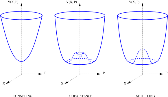
Figure 7.11: Schematic representation of the effective potentials for the three operating regimes.

Elimination of the fast dynamics

The starting point are the Klein-Kramers equations for the SDQS that we rewrite symmetrized by shifting the coordinates origin to $d/2$:

$$\begin{split}\frac{\partial W_{00}}{\partial t}=&\left[m\omega^{2}\left(q+\frac{d}{2}\right)\frac{\partial}{\partial p}-\frac{p}{m}\frac{\partial}{\partial q}+\gamma\frac{\partial}{\partial p}p+\gamma m\hbar\omega\left(n_{B}+\frac{1}{2}\right)\frac{\partial^{2}}{\partial p^{2}}\right]W_{00}\\ &+\Gamma_{R}e^{2q/\lambda}W_{11}-\Gamma_{L}e^{-2q/\lambda}\sum_{n=0}^{\infty}\frac{(-1)^{n}}{(2n)!}\left(\frac{\hbar}{\lambda}\right)^{2n}\frac{\partial^{2n}W_{00}}{\partial p^{2n}}\\ \frac{\partial W_{11}}{\partial t}=&\left[m\omega^{2}\left(q-\frac{d}{2}\right)\frac{\partial}{\partial p}-\frac{p}{m}\frac{\partial}{\partial q}+\gamma\frac{\partial}{\partial p}p+\gamma m\hbar\omega\left(n_{B}+\frac{1}{2}\right)\frac{\partial^{2}}{\partial p^{2}}\right]W_{11}\\ &+\Gamma_{L}e^{-2q/\lambda}W_{00}-\Gamma_{R}e^{2q/\lambda}\sum_{n=0}^{\infty}\frac{(-1)^{n}}{(2n)!}\left(\frac{\hbar}{\lambda}\right)^{2n}\frac{\partial^{2n}W_{11}}{\partial p^{2n}}\end{split}$$ (7.80)

One by one we will now get rid of the variables that due to their fast dynamics are not relevant for the description of the coexistence regime. In equations (7.80) we describe the electrical state of the dot as empty or charged. We shift to the description in terms of state $+$ and state $-$ with the definition:

$$W_{+}=W_{00}+W_{11},\quad W_{-}=W_{00}-W_{11}$$ (7.81)

In terms of these new Wigner functions the Klein-Kramers equations read:

$$\begin{split}\partial_{t}W_{+}&=\{H_{\rm osc},W_{+}\}_{P}+\mathcal{L}_{1}W_{+}+\mathcal{L}_{2}W_{-}\\ \partial_{t}W_{-}&=\{H_{\rm osc},W_{-}\}_{P}+(\mathcal{L}_{1}+\Gamma_{+})W_{-}+(\mathcal{L}_{2}+\Gamma_{-})W_{+}\\ \end{split}$$ (7.82)

where

$$\begin{split}\Gamma_{+}&=\Gamma_{R}e^{2q/\lambda}+\Gamma_{L}e^{-2q/\lambda}\\ \Gamma_{-}&=\Gamma_{R}e^{2q/\lambda}-\Gamma_{L}e^{-2q/\lambda}\\ \mathcal{L}_{1}&=\gamma\partial_{p}p+\gamma m\hbar\omega\left(n_{B}+\frac{1}{2}\right)\partial^{2}_{p}-\frac{\Gamma_{+}}{2}\sum_{n=1}^{\infty}\frac{1}{2n!}\left(\frac{\hbar}{i\lambda}\right)^{2n}\partial^{2n}_{p}\\ \mathcal{L}_{2}&=\frac{e\mathcal{E}}{2}\frac{\partial}{\partial p}+\frac{\Gamma_{-}}{2}\sum_{n=1}^{\infty}\frac{1}{2n!}\left(\frac{\hbar}{i\lambda}\right)^{2n}\partial_{p}^{2n}\end{split}$$ (7.83)

The symbol $\{\bullet,\bullet\}_{P}$ represents the Poisson brackets and we have introduced for the partial derivatives the short notation $\partial_{x}\equiv\frac{\partial}{\partial x}$. It is useful for the calculation of the effective potential to treat position and momentum on equal footing. For this reason we introduce the adimensional variables:

$$X=\frac{q}{\lambda},\quad P=\frac{p}{m\lambda\omega},\quad\tau=t\omega$$ (7.84)

The general structure of the equations (7.82) remains unchanged but the Liouvilleans and the $\Gamma$ functions take the form:

$$\begin{split}\Gamma_{+}&=\frac{\Gamma_{R}}{\omega}e^{2X}+\frac{\Gamma_{L}}{\omega}e^{-2X}\\ \Gamma_{-}&=\frac{\Gamma_{R}}{\omega}e^{2X}-\frac{\Gamma_{L}}{\omega}e^{-2X}\\ \mathcal{L}_{1}&=\frac{\gamma}{\omega}\partial_{P}P+\frac{\gamma}{\omega}\left(\frac{x_{0}}{\lambda}\right)^{2}\left(n_{B}+\frac{1}{2}\right)\partial^{2}_{P}-\frac{\Gamma_{+}}{2}\sum_{n=1}^{\infty}\frac{(-1)^{n}}{2n!}\left(\frac{x_{0}}{\lambda}\right)^{4n}\partial^{2n}_{P}\\ \mathcal{L}_{2}&=\frac{d}{2\lambda}\partial_{P}+\frac{\Gamma_{-}}{2}\sum_{n=1}^{\infty}\frac{(-1)^{n}}{2n!}\left(\frac{x_{0}}{\lambda}\right)^{4n}\partial_{P}^{2n}\end{split}$$ (7.85)

Since in the following we will assume the “classical” limit of a tunneling length much larger than the zero point uncertainty in the position, only the first term of the sums that appears in the definition of $\mathcal{L}_{1}$ and $\mathcal{L}_{2}$ will be kept. Following Fedorets et al. [9] we also introduce polar coordinates:

$$X=A\sin\phi,\quad P=A\cos\phi$$ (7.86)

The equations (7.82) are transformed into:

$$\begin{split}\partial_{\tau}W_{+}&=(-\partial_{\phi}+\mathcal{L}_{1})W_{+}+\mathcal{L}_{2}W_{-}\\ \partial_{\tau}W_{-}&=(-\partial_{\phi}+\mathcal{L}_{1}-\Gamma_{+})W_{-}+(\mathcal{L}_{2}+\Gamma_{-})W_{+}\\ \end{split}$$ (7.87)

It is interesting to note that the Poisson brackets for the harmonic oscillator reduce in the polar coordinates to $-\partial_{\phi}$ since there is no amplitude dynamics in the phase space. The $\Gamma$ functions now read:

$$\begin{split}\Gamma_{+}&=\frac{\Gamma_{R}}{\omega}e^{2A\sin\phi}+\frac{\Gamma_{L}}{\omega}e^{-2A\sin\phi}\\ \Gamma_{-}&=\frac{\Gamma_{R}}{\omega}e^{2A\sin\phi}-\frac{\Gamma_{L}}{\omega}e^{-2A\sin\phi}\end{split}$$ (7.88)

For the transformation of the Liouvilleans $\mathcal{L}_{1,2}$ we used the polar coordinate representation of the following differential operators:

$$\begin{split}\partial_{P}=&-\frac{\sin\phi}{A}\partial_{\phi}+\cos\phi\partial_{A}\\ =&\frac{1}{A}\cos\phi\partial_{A}A-\frac{1}{A}\partial_{\phi}\sin\phi\\ \partial^{2}_{P}=&\frac{2}{A^{2}}\cos\phi\sin\phi\partial_{\phi}+\frac{\sin^{2}\phi}{A}\partial_{A}+\frac{\sin^{2}\phi}{A^{2}}\partial^{2}_{\phi}\\ &-\frac{2}{A}\sin\phi\cos\phi\partial^{2}_{A\phi}+\cos^{2}\phi\partial^{2}_{A}\\ =&\frac{1}{A}\cos^{2}\phi\partial^{2}_{A}A-\frac{2}{A}\partial^{2}_{A\phi}\sin\phi\cos\phi+\frac{1}{A^{2}}\partial^{2}_{\phi}\sin^{2}\phi\\ &-\frac{1}{A}\partial_{A}\sin^{2}\phi-\frac{2}{A^{2}}\partial_{\phi}\cos\phi\sin\phi\\ \partial_{P}P=&\frac{1}{A}\cos^{2}\phi\partial_{A}A^{2}-\partial_{\phi}\sin\phi\cos\phi\\ =&1-\sin\phi\cos\phi\partial_{\phi}+\cos^{2}\phi A\partial_{A}\end{split}$$ (7.89)

where $\partial^{2}_{A\phi}\equiv\frac{\partial^{2}}{\partial A\partial\phi}$. The two different forms (partial differential operator $\partial_{A}$ and/or $\partial_{\phi}$ to the extreme left or right) that for the moment seem redundant will be very useful in the derivation of the effective potential.

We now start to make approximations on the system of equations (7.87) with the main idea of eliminating the fast irrelevant variables. We know that eventually the density operators $\sigma_{ii}$ that describe the system will reach a stationary state. In absence of the harmonic oscillator the state $+$ would be fixed by the trace sum rule and the state $-$ would relax to zero on a time scale fixed by the tunneling rates. We assume that also in the presence of the mechanical degree of freedom the relaxation dynamics of the $|-\rangle$ state is much faster than the one of the $|+\rangle$ state. We set $\partial_{\tau}W_{-}$ to zero in the second equation of (7.87) and formally solve the equation for $W_{-}$. We insert the result in the first equation of (7.87) and obtain a closed equation for the (total) Wigner function $W_{+}$:

$$\begin{split}\partial_{\tau}W_{+}&=[-\partial_{\phi}+\underbrace{\mathcal{L}_{1}+\mathcal{L}_{2}(1-\hat{G}_{0}\mathcal{L}_{1})^{-1}\hat{G}_{0}(\mathcal{L}_{2}+\Gamma_{-})}_{\displaystyle\mathcal{L}_{+}}]W_{+}\\ \end{split}$$ (7.90)

where $\hat{G}_{0}\equiv(\partial_{\phi}+\Gamma_{+})^{-1}$ and we also define the (super)operator $\mathcal{L}_{+}$. At this point the detailed information about the charge state of the oscillating dot is integrated out, but the equation (7.90) still takes the fast phase dynamics into account. Since we are interested only in the amplitude dynamics (the slowest in the coexistence regime) we introduce the projector $\mathcal{P}_{\phi}$ that averages over the phase and its orthogonal complement $\mathcal{Q}_{\phi}=1-\mathcal{P}_{\phi}$:

$$\mathcal{P}_{\phi}[\bullet]=\frac{1}{2\pi}\int_{0}^{2\pi}d\phi\bullet$$ (7.91)

Using these two operators we decompose the Wigner distribution function into:

$$W_{+}=\mathcal{P}W_{+}+\mathcal{Q}W_{+}=\bar{W}_{+}+\tilde{W}_{+}$$ (7.92)

We apply the same projectors also to the equation (7.90) and we obtain the set of coupled partial (integro-)differential equations:

$$\begin{split}\partial_{\tau}\bar{W}_{+}&=\mathcal{P}_{\phi}\mathcal{L}_{+}\bar{W}_{+}+\mathcal{P}_{\phi}\mathcal{L}_{+}\tilde{W}_{+}\\ \partial_{\tau}\tilde{W}_{+}&=[-\partial_{\phi}+\mathcal{Q}_{\phi}\mathcal{L}_{+}]\tilde{W}_{+}+\mathcal{Q}_{\phi}\mathcal{L}_{+}\bar{W}_{+}\end{split}$$ (7.93)

where we have used the properties:

$$\begin{split}&\mathcal{P}_{\phi}\partial_{\phi}=0\\ &\mathcal{Q}_{\phi}\partial_{\phi}=\partial_{\phi}\mathcal{Q}_{\phi}=\partial_{\phi}\end{split}$$ (7.94)

which is readily demonstrated since all the distributions involved are periodic functions of $\phi$. We now assume that the phase relaxation time that governs the dynamics of the phase-dependent distribution $\tilde{W}_{+}$ is much shorter than the amplitude relaxation time of the distribution $W_{+}$ . We then set $\partial_{\tau}\tilde{W}_{+}=0$ in the second equation of (7.93), solve it for $\tilde{W}_{+}$ and insert the result in the first equation. The result is a closed equation for the (quasi)probability distribution function $\bar{W}_{+}$:

$$\partial_{\tau}\bar{W}_{+}=\mathcal{P}_{\phi}\mathcal{L}_{+}[1+(1-\hat{g}_{0}\mathcal{Q}_{\phi}\mathcal{L}_{+})^{-1}\hat{g}_{0}\mathcal{Q}_{\phi}\mathcal{L}_{+}]\bar{W}_{+}$$ (7.95)

where $\hat{g}_{0}\equiv(\partial_{\phi})^{-1}$. We notice that the operator $\hat{g}_{0}$ is in the equations always following the projector $\mathcal{Q}_{\phi}$. This combination of operators ensures us as an output a periodic function in the variable $\phi$.

Small parameters expansion

We believe that equation (7.95) contains the relevant dynamics of the SDQS in the coexistence regime, but, despite all the approximations already introduced the problem still looks untractable. Again following the already mentioned work by Fedorets et al. [9] we consider the perturbation expansion of (7.95) in the “small parameters”:

$$\frac{d}{\lambda},\quad\left(\frac{x_{0}}{\lambda}\right)^{2},\quad\frac{\gamma}{\omega}\ll 1$$ (7.96)

These three inequalities describe a limit often encountered in this thesis and they correspond respectively to the three physical assumptions:

1. The external electrostatic force is a small perturbation of the harmonic oscillator restoring force in terms of the sensitivity to displacement of the tunneling rates. This ensures a quasi oscillator-independent treatment of the tunneling regime.

2. The tunneling length is big compared to the zero point fluctuations. Since the oscillator dynamics for the shuttling (and then partially also for the coexistence) regime happens on the scale of the tunneling length, this condition ensures a quasi-classical behaviour of the harmonic oscillator.

3. The coupling of the oscillator to the thermal bath is weak and the oscillator dynamics is under-damped.

We want to expand the equation (7.95) up to second order in the three small parameters (7.96). To proceed systematically we first notice that they appear at least to first order in the Liouvilleans $\mathcal{L}_{1}$ and $\mathcal{L}_{2}$ and thus also in the operator $\mathcal{L}_{+}$. We can then safely expand (7.95) up to second order in $\mathcal{L}_{+}$ without missing any desired term:

$$\partial_{\tau}\bar{W}_{+}\approx\mathcal{P}_{\phi}\mathcal{L}_{+}[1+\hat{g}_{0}\mathcal{Q}_{\phi}\mathcal{L}_{+}]\bar{W}_{+}$$ (7.97)

Using the definition of $\mathcal{L}_{+}$ contained in (7.90) we now expand this last equation up to second order in $\mathcal{L}_{1}$ and $\mathcal{L}_{2}$:

$$\begin{split}\partial_{\tau}\bar{W}_{+}\approx[&\mathcal{P}_{\phi}\mathcal{L}_{1}+\mathcal{P}_{\phi}\mathcal{L}_{2}\hat{G}_{0}\Gamma_{-}\\ +&\mathcal{P}_{\phi}\mathcal{L}_{2}\hat{G}_{0}\mathcal{L}_{1}\hat{G}_{0}\Gamma_{-}+\mathcal{P}_{\phi}\mathcal{L}_{2}\hat{G}_{0}\mathcal{L}_{2}\\ +&\mathcal{P}_{\phi}\mathcal{L}_{1}\hat{g}_{0}\mathcal{Q}_{\phi}\mathcal{L}_{1}+\mathcal{P}_{\phi}\mathcal{L}_{2}\hat{G}_{0}\Gamma_{-}\hat{g}_{0}\mathcal{Q}_{\phi}\mathcal{L}_{2}\hat{G}_{0}\Gamma_{-}\\ +&\mathcal{P}_{\phi}\mathcal{L}_{1}\hat{g}_{0}\mathcal{Q}_{\phi}\mathcal{L}_{2}\hat{G}_{0}\Gamma_{-}+\mathcal{P}_{\phi}\mathcal{L}_{2}\hat{G}_{0}\Gamma_{-}\hat{g}_{0}\mathcal{Q}_{\phi}\mathcal{L}_{1}]\bar{W}_{+}\end{split}$$ (7.98)

The last step is to consider within the equation (7.98) only the contributions up to second order in the expansion parameters (7.96). In the definition of the Liouvilleans in the adimensional form (7.85) we note that each of the small parameters (7.96) is associated with a differential operator $\partial_{P}$. We then average out the phase variable from the equations. We thus expect the second order expansion in the small parameters (7.96) to be of second order in the differential operator $\partial_{A}$. More precisely the expansion takes the form:

$$\partial_{\tau}\bar{W}_{+}(A,\tau)=\frac{1}{A}\partial_{A}A[V^{\prime}(A)+D(A)\partial_{A}]\bar{W}_{+}(A,\tau)$$ (7.99)

where $V^{\prime}(A)=\frac{d}{dA}V(A)$ and $D(A)$ are given functions of A. Before calculating explicitly all the different contributions that compose the functions $V^{\prime}$ and $D$ we want to explore the consequences of the formulation of the Klein-Kramers equations (7.80) in the form (7.99). The stationary solution of the equation (7.99) reads:

$$\bar{W}_{+}^{\rm stat}(A)=\frac{1}{\mathcal{Z}}\exp\left(-\int_{0}^{A}dA^{\prime}\frac{V^{\prime}(A^{\prime})}{D(A^{\prime})}\right)$$ (7.100)

where $\mathcal{Z}$ is the normalization that ensures the integral of the phase-space distribution to be unity: $\int_{0}^{\infty}dA^{\prime}2\pi A^{\prime}\bar{W}_{+}^{\rm stat}(A^{\prime})=1$. The equation (7.99) is identical to the Fokker-Planck equation for a particle in the bidimensional rotationally invariant potential $V$ (see figure 7.11) with stochastic forces described by the (position dependent) diffusion coefficient $D$.

All the differential operators acting on $\bar{W}_{+}$ in (7.98) are at maximum of second order in $\partial_{A}$. In order to obtain Eq. (7.99) we substitute into (7.98) the definition of $\mathcal{L}_{1}$ and $\mathcal{L}_{2}$ and we “push” the differential operator $\partial_{A}$ all the way towards the left or the right in the sequence of operators acting on $\bar{W}_{+}$. All the components in which we are left with only one $\partial_{A}$ operator on the right define the effective potential $V$. All the others have the second $\partial_{A}$ on the extreme right and define $D(A)$. All contributions to the effective potential $V$ and diffusion coefficient $D$ can be grouped according to the power of the small parameters that they contain.

$$\begin{split}V^{\prime}(A)&=\frac{\gamma}{\omega}\frac{A}{2}+\frac{d}{2\lambda}\alpha_{0}(A)+\left(\frac{x_{0}}{\lambda}\right)^{4}\alpha_{1}(A)+\left(\frac{d}{2\lambda}\right)^{2}\alpha_{2}(A)+\frac{\gamma}{\omega}\frac{d}{2\lambda}\alpha_{3}(A)\\ D(A)&=\frac{\gamma}{\omega}\left(\frac{x_{0}}{\lambda}\right)^{2}\frac{1}{2}\left(n_{B}+\frac{1}{2}\right)+\left(\frac{x_{0}}{\lambda}\right)^{4}\beta_{1}(A)+\left(\frac{d}{2\lambda}\right)^{2}\beta_{2}(A)+\frac{\gamma}{\omega}\frac{d}{2\lambda}\beta_{3}(A)\end{split}$$ (7.101)

where the $\alpha$ functions read:

$$\begin{split}\alpha_{0}=&\mathcal{P}_{\phi}\cos\phi\hat{G}_{0}\Gamma_{-}\\ \alpha_{1}=&-\frac{1}{4}\mathcal{P}_{\phi}\cos\phi\Gamma_{-}\partial_{P}(\hat{G}_{0}\Gamma_{-})\\ \alpha_{2}=&\mathcal{P}_{\phi}\cos\phi\hat{G}_{0}\Gamma_{-}\hat{g}_{0}\mathcal{Q}_{\phi}\partial_{P}(\hat{G}_{0}\Gamma_{-})\\ \alpha_{3}=&\mathcal{P}_{\phi}\cos\phi\Big{[}\hat{G}_{0}^{2}\Gamma_{-}+A\hat{G}_{0}\partial_{P}(\hat{G}_{0}\Gamma_{-})-\frac{A}{2}\sin\phi\partial_{P}(\hat{G}_{0}\Gamma_{-})\Big{]}\end{split}$$ (7.102)

and the $\beta$’s can be written as:

$$\begin{split}\beta_{1}=&\frac{1}{4}\mathcal{P}_{\phi}\cos^{2}\phi\Big{[}\Gamma_{+}-\Gamma_{-}\hat{G}_{0}\Gamma_{-}\Big{]}\\ \beta_{2}=&\mathcal{P}_{\phi}\cos\phi\Big{[}\hat{G}_{0}\cos\phi+\hat{G}_{0}\Gamma_{-}\hat{g}_{0}\mathcal{Q}_{\phi}\cos\phi\hat{G}_{0}\Gamma_{-}\Big{]}\\ \beta_{3}=&A\mathcal{P}_{\phi}\cos\phi\Big{[}\hat{G}_{0}\cos^{2}\phi\hat{G}_{0}\Gamma_{-}+\frac{1}{4}\hat{G}_{0}\Gamma_{-}\sin 2\phi-\frac{1}{4}\sin 2\phi\hat{G}_{0}\Gamma_{-}\Big{]}\\ \end{split}$$ (7.103)

In the expression above the $\phi$ variable disappears on the RHS when we apply the projector $\mathcal{P}_{\phi}$. We have kept the somehow mixed notation with the differential operator $\partial_{P}$ to keep the notation lighter. In general the operators are acting on all what is on their right. Otherwise parentheses are limiting their range of action (see for example $\partial_{P}$ and in $\alpha_{1}$). As examples of the arguments that appear in the calculation of the $\alpha$ and $\beta$ functions we give first the derivation of a “missing” contribution, then we explicitly derive $\alpha_{3}$ and $\beta_{3}$.

Some second order contributions in the parameters (7.96) simply do not appear in the final expansions because the small parameter combinations which they represent is not present. The contribution in $\left(\frac{\gamma}{\omega}\right)^{2}$ instead is formally there but vanishes identically. From the expansion in terms of the operators $\mathcal{L}_{1}$ and $\mathcal{L}_{2}$ this contribution reads:

$$\mathcal{L}_{\gamma\gamma}\equiv\mathcal{P}_{\phi}\partial_{P}P\hat{g}_{0}\mathcal{Q}_{\phi}\partial_{P}P$$ (7.104)

We insert the polar coordinate expressions for the differential operators $\partial_{P}P$ (see Eq. 7.89) choosing the left operator form for the first and the right form for the second and we obtain:

$$\mathcal{L}_{\gamma\gamma}=\frac{1}{A}\partial_{A}A^{2}\mathcal{P}_{\phi}\cos^{2}\phi\hat{g}_{0}\mathcal{Q}(1+\cos^{2}\phi A\partial_{A})$$ (7.105)

where we have used also the fact that the operator is applied to $\bar{W}_{+}$ which does not depend on $\phi$. Remembering that $\mathcal{Q}_{\phi}=1-\mathcal{P}_{\phi}$ and $\hat{g}_{0}$ is the indefinite integral in the variable $\phi$ we conclude the calculation:

$$\begin{split}\mathcal{L}_{\gamma\gamma}&=\frac{1}{A}\partial_{A}A^{2}\mathcal{P}_{\phi}\cos^{2}\phi\hat{g}_{0}\left(\cos^{2}\phi-\frac{1}{2}\right)A\partial_{A}\\ &=\frac{1}{2A}\partial_{A}A^{2}\mathcal{P}_{\phi}\cos^{3}\phi\sin\phi A\partial_{A}=0\end{split}$$ (7.106)

The functions $\alpha_{3}$ and $\beta_{3}$ are both derived from the contribution $\frac{\gamma}{\omega}\frac{d}{2\lambda}$ of the small parameter expansion (7.98). The corresponding Liouvillean reads:

$$\begin{split}\mathcal{L}_{\gamma d}=&\mathcal{P}_{\phi}\partial_{P}\hat{G}_{0}\partial_{P}P\hat{G}_{0}\Gamma_{-}+\\ &\mathcal{P}_{\phi}\partial_{P}P\hat{g}_{0}\mathcal{Q}_{\phi}\partial_{P}\hat{G}_{0}\Gamma_{-}+\\ &\mathcal{P}_{\phi}\partial_{P}\hat{G}_{0}\Gamma_{-}\hat{g}_{0}\mathcal{Q}_{\phi}\partial_{P}P\end{split}$$ (7.107)

We now use polar coordinates and take into account that the Liouvillean is applied to a function $\bar{W}_{+}$ independent of the variable $\phi$. We obtain:

$$\begin{split}\mathcal{L}_{\gamma d}=\frac{1}{A}\partial_{A}A&\mathcal{P}_{\phi}\cos\phi\\ \Big{[}&\hat{G}_{0}^{2}\Gamma_{-}+\hat{G}_{0}A\cos\phi\partial_{P}(\hat{G}_{0}\Gamma_{-})+\hat{G}_{0}A\cos^{2}\phi\hat{G}_{0}\Gamma_{-}\partial_{A}+\\ &A\cos\phi\hat{g}_{0}\mathcal{Q}_{\phi}\partial_{P}(\hat{G}_{0}\Gamma_{-})+A\cos\phi\hat{g}_{0}\mathcal{Q}_{\phi}\cos\phi\hat{G}_{0}\Gamma_{-}\partial_{A}+\\ &\hat{G}_{0}\Gamma_{-}\hat{g}_{0}\mathcal{Q}_{\phi}A\cos^{2}\phi\partial_{A}\Big{]}\end{split}$$ (7.108)

The $\alpha_{3}$ and $\beta_{3}$ contributions can be split to obtain:

$$\begin{split}\mathcal{L}_{\gamma d}=&\frac{1}{A}\partial_{A}A\left\{\mathcal{P}_{\phi}\cos\phi\Big{[}\hat{G}_{0}^{2}\Gamma_{-}+A\hat{G}_{0}\partial_{P}(\hat{G}_{0}\Gamma_{-})-\frac{A}{2}\sin\phi\partial_{P}(\hat{G}_{0}\Gamma_{-})\Big{]}\right\}+\\ &\frac{1}{A}\partial_{A}A\left\{\mathcal{P}_{\phi}\cos\phi\Big{[}\hat{G}_{0}\cos^{2}\phi\hat{G}_{0}\Gamma_{-}+\frac{1}{4}\hat{G}_{0}\Gamma_{-}\sin 2\phi-\frac{1}{4}\sin 2\phi\hat{G}_{0}\Gamma_{-}\Big{]}\right\}\partial_{A}\end{split}$$ (7.109)

Since we have projected out the phase $\phi$ we are effectively working in a one-dimensional phase space given by the amplitude $A$. Equation (7.99) though is not as it is a Kramers equation for a single variable. This is related to the fact that also the distribution $\bar{W}_{+}$ is not the amplitude distribution function, but, so to speak, a cut at fixed phase of a two dimensional rotationally invariant distribution. The difference is a geometrical factor $A$ that it turns out is also simplifying the equation. We define the amplitude probability distribution $\mathcal{W}(A,\tau)=A\bar{W}_{+}(A,\tau)$ and insert this definition in equation (7.99). We obtain:

$$\begin{split}\partial_{\tau}\mathcal{W}(A,\tau)&=\partial_{A}A[V^{\prime}(A)+D(A)\partial_{A}]\frac{1}{A}\mathcal{W}(A,\tau)\\ &=\partial_{A}[\mathcal{V}^{\prime}(A)+D(A)\partial_{A}]\mathcal{W}(A,\tau)\end{split}$$ (7.110)

where we have defined the geometrically corrected potential

$$\mathcal{V}(A)=V(A)-\int_{A_{0}}^{A}\!\!\frac{D(A^{\prime})}{A^{\prime}}dA^{\prime}$$ (7.111)

which for an amplitude independent diffusion coefficient gives a corrected potential logarithmically divergent in the origin. The integration extremal is arbitrary and reflects the arbitrary constant in the definition of the potential. The equation (7.110) is the one-dimensional Kramers equation that constitutes the starting point for the calculation of the switching rates that characterize the coexistence regime.

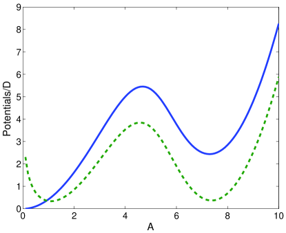
Figure 7.12: Example of the potential $V$ (full) and the geometrically corrected potential $\mathcal{V}$ (dashed) for the SDQS in the coexistence regime. Notice for the corrected potential the logarithmic divergence in the origin.

Evaluation of the $\alpha_{i}$ and $\beta_{i}$ functions

We evaluate the $\alpha_{i}$ and $\beta_{i}$ functions numerically. Fortunately there is a rather natural discretization of the operators that compose the $\alpha$ and $\beta$. This discretization is given by the operator $\mathcal{P}_{\phi}\cos\phi$ that opens the operator string of all the components and that can be considered as a sort of Fourier transform of the function that follows. We specify better the concept and the method by reducing explicitly to the “numerical form” the contributions $\alpha_{0}$ and $\alpha_{2}$:

$$\begin{split}\alpha_{0}=&\mathcal{P}_{\phi}\cos\phi\hat{G}_{0}\Gamma_{-}\\ \alpha_{2}=&\mathcal{P}_{\phi}\cos\phi\hat{G}_{0}\Gamma_{-}\hat{g}_{0}\mathcal{Q}_{\phi}\partial_{P}(\hat{G}_{0}\Gamma_{-})\\ \end{split}$$ (7.112)

where we remind $\hat{G}_{0}=(\partial_{\phi}+\Gamma_{+})^{-1}$. We define the function $G(A,\phi)\equiv\hat{G}_{0}\Gamma_{-}(A,\phi)$. If $\tilde{G}_{n}(A)$ is the discrete Fourier transform of $G$ (periodic function of $\phi$)

$$\tilde{G}_{n}(A)=\frac{1}{2\pi}\int_{0}^{2\pi}G(A,\phi)e^{in\phi}$$ (7.113)

with $n\in\mathbb{Z}$, then we can easily recognize the Fourier transform in the definition of $\alpha_{0}$ and write:

$$\alpha_{0}(A)=\frac{1}{2}(\tilde{G}_{1}+\tilde{G}_{-1})$$ (7.114)

We still need to identify the structure of the functions $\tilde{G}_{n}(A)$. It is useful for this purpose to calculate the Fourier transform of the functions $\Gamma_{+}$ and $\Gamma_{-}$ and define the vectors $\tilde{\bar{\Gamma}}_{+}$ and $\tilde{\bar{\Gamma}}_{-}$ whose components are:

$$\begin{split}(\tilde{\bar{\Gamma}}_{+})_{n}=\frac{\Gamma}{\omega}[J_{n}(-2iA)+J_{n}(2iA)]\\ (\tilde{\bar{\Gamma}}_{-})_{n}=\frac{\Gamma}{\omega}[J_{n}(-2iA)-J_{n}(2iA)]\end{split}$$ (7.115)

where we have assumed for simplicity that $\Gamma_{L}=\Gamma_{R}=\Gamma$ and the Bessel function $J_{n}(z)$ is defined by:

$$J_{n}(z)=\frac{1}{2\pi}\int_{0}^{2\pi}e^{in\phi+iz\sin\phi}d\phi$$ (7.116)

At the operator level we can write:

$$\Gamma_{-}(A,\phi)=[\partial_{\phi}+\Gamma_{+}(A,\phi)]G(A,\phi)$$ (7.117)

We take the Fourier transform in $\phi$ on both sides and we obtain:

$$(\tilde{\bar{\Gamma}}_{-})_{n}=\sum_{m=-\infty}^{\infty}[\underbrace{in\delta_{mn}+(\tilde{\bar{\bar{\Gamma}}}_{+})_{nm}}_{\displaystyle M_{nm}}]\tilde{G}_{m}$$ (7.118)

where we have defined the matrix $(\tilde{\bar{\bar{\Gamma}}}_{+})_{nm}\equiv(\tilde{\bar{\Gamma}}_{+})_{n-m}$ and the matrix $M$. Finally we also define the Fourier transform of the cosine $\bar{C}=[\ldots,\frac{1}{2},0,\frac{1}{2},\ldots]^{T}$ with the $1/2$ in position $\pm 1$ and we write the $\alpha_{0}$ function in the compact numerical form:

$$\alpha_{0}=(\bar{C},M^{-1}\tilde{\bar{\Gamma}}_{-})$$ (7.119)

where the symbol $(\bullet,\bullet)$ indicates the scalar product between the two vectors. All the vectors must be truncated in the numerical evaluation, but fortunately the Bessel functions $J_{n}$ decay fast with $n$ and typically we verified numerical convergence taking only 40 terms around the zero position of the discrete Fourier transform “momentum space”.

If the derivation of the numerical form for $\alpha_{0}$ is revealing the spirit of the calculation, the $\alpha_{2}$ case contains instead some of the typical “tricks”. We start from the definition (7.112) and express the differential operator $\partial_{P}$ in polar coordinates. We obtain:

$$\alpha_{2}=\mathcal{P}_{\phi}\cos\phi\hat{G}_{0}\Gamma_{-}\hat{g}_{0}\mathcal{Q}_{\phi}\left(-\frac{\sin\phi}{A}\partial_{\phi}+\cos\phi\partial_{A}\right)\hat{G}_{0}\Gamma_{-}$$ (7.120)

We absorb the partial derivative $\partial_{\phi}$ with the identification:

$$\partial_{\phi}=\hat{G}_{0}^{-1}-\Gamma_{+}$$ (7.121)

Another important element is the combination $\hat{g}_{0}\mathcal{Q}_{\phi}$. It is important to study the Fourier transform of such an operator. Since $\hat{g}_{0}=(\partial_{\phi})^{-1}$ we obtain:

$$(\hat{g}_{0})_{mn}=-\frac{i}{n}\delta_{nm}$$ (7.122)

The singularity for $n=0$ is cured by the projector $\mathcal{Q}_{\phi}$ that removes the $0^{\rm th}$ component in the Fourier transform of the vector on which it is acting. We call for this reason the combination $\hat{g}_{0}\mathcal{Q}_{\phi}$ the pseudoinverse of the differential operator $\partial_{\phi}$ and we use the symbol $(\partial_{\phi}^{-1})_{PS}$.

The last problem that must be faced is the differential operator $\partial_{A}$ that we always encounter in the expression $\partial_{A}G$. Using the definition of $G$ and the results obtained in the evaluation of $\alpha_{0}$ we can write:

$$\partial_{A}\tilde{G}=M^{-1}\partial_{A}\tilde{\bar{\Gamma}}_{-}-M^{-1}\partial_{A}(M)M^{-1}\tilde{\bar{\Gamma}}_{-}$$ (7.123)

For the matrix $M$ and the vector $\tilde{\bar{\Gamma}}_{-}$ we have the explicit formulation in terms of the Bessel functions. Using the recursive relation between the functions $J$ and their derivatives

$$\partial_{z}J_{n}(z)=\frac{1}{2}[J_{n-1}(z)-J_{n+1}(z)]$$ (7.124)

we obtain:

$$\begin{split}(\partial_{A}M)_{mn}=\frac{i\Gamma}{\omega}[&J_{n-m+1}(-2iA)-J_{n-m-1}(-2iA)\\ -&J_{n-m+1}(+2iA)+J_{n-m-1}(+2iA)]\\ (\partial_{A}\tilde{\bar{\Gamma}}_{-})_{n}=\frac{i\Gamma}{\omega}[&J_{n+1}(-2iA)-J_{n-1}(-2iA)\\ +&J_{n+1}(+2iA)-J_{n-1}(+2iA)]=(\partial_{A}\tilde{\bar{\bar{\Gamma}}}_{-})_{n0}\end{split}$$ (7.125)

The “numerical form” of the function $\alpha_{2}$ reads:

$$\begin{split}\alpha_{2}=-\frac{1}{A}\Big{(}\bar{C},\,&M^{-1}\tilde{\bar{\bar{\Gamma}}}_{-}(\partial_{\phi})^{-1}_{PS}\big{(}\bar{\bar{S}}\tilde{\bar{\Gamma}}_{-}-\bar{\bar{S}}\tilde{\bar{\bar{\Gamma}}}_{+}\tilde{G}\\ &-A\bar{\bar{C}}M^{-1}(\partial_{A}\tilde{\bar{\Gamma}}_{-}-\partial_{A}(M)\tilde{G})\big{)}\Big{)}\end{split}$$ (7.126)

where we have also introduced the $\sin$ and $\cos$ Fourier matrices:

$$\bar{\bar{S}}=\frac{1}{2i}\begin{pmatrix}\phantom{-}0&\phantom{-}1&0&\cdots\\ -1&\phantom{-}0&1&\cdots\\ \phantom{-}0&-1&0&\ddots\\ \phantom{-}\vdots&\phantom{-}\vdots&\ddots&\ddots\\ \end{pmatrix},\quad\bar{\bar{C}}=\frac{1}{2}\begin{pmatrix}0&1&0&\cdots\\ 1&0&1&\cdots\\ 0&1&0&\ddots\\ \vdots&\vdots&\ddots&\ddots\\ \end{pmatrix}$$ (7.127)

The other $\alpha$ and $\beta$ functions are evaluated in a similar way and the calculations involved do not present any further complication.

7.3.3 Switching Rates

We have proven in section 7.3.2 that the SDQS dynamics in the coexistence regime can be described by a Kramers equation for the amplitude probability distribution $\mathcal{W}$ with a given potential $\mathcal{V(A)}$ and diffusion “constant” $D(A)$. We then dedicated the last section to describe an affordable and reliable numerical evaluation of the $\alpha$ and $\beta$ functions that appear in the definition of the potential and diffusion constant. We are now able to identify completely the SDQS operating in the coexistence regime as a particular realization of the model for a dichotomous process between current modes presented in section 7.3.1. The shuttling and tunneling regimes with their characteristic currents are the two modes. Within the framework of the Kramers escape time theory we can now calculate the switching rates between these two modes.

The effective potential $\mathcal{V}$ that we obtained has for parameters that correspond to the coexistence regime, a typical double well bistable shape (Fig. 7.12). We assume for a while the diffusion constant to be independent of the amplitude $A$. In this approximation the stationary solution of the equation (7.110) reads:

$$\mathcal{W}^{\rm stat}(A)=\frac{1}{\mathcal{Z}}\exp\left(-\frac{\mathcal{V}(A)}{D}\right)$$ (7.128)

where $\mathcal{Z}$ is the normalization $\mathcal{Z}=\int_{0}^{\infty}\mathcal{W}^{\rm stat}(A)dA$. The probability distribution is concentrated around the minima of the potential and has a minimum in correspondence of the potential barrier. If this potential barrier is high enough (i.e. $\mathcal{V}_{\rm max}-\mathcal{V}_{\rm min}\gg D$) we clearly identify two distinct states with definite average amplitude: the lower amplitude state corresponding to the tunneling regime and the higher to the shuttling (see fig. 7.13).

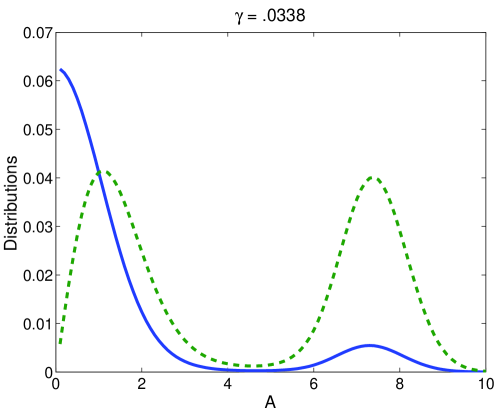
Figure 7.13: Example of the stationary distribution $\bar{W}_{+}^{\rm stat}$ (full) and the amplitude distribution $\mathcal{W}^{\rm stat}$ (dashed) for the SDQS in the coexistence regime. The tunneling and shuttling states are in both cases well separated.

The Kramers equation (7.110) describes the coexistence regime of a SDQS by mapping it into a classical model for a particle moving in a bistable potential $\mathcal{V}$ with random forces described by the diffusion constant $D$. It is this random force that allows the particle to overcome the barrier and jump between the two minima with definite rates. These rates are in the model for the SDQS the switching rates between the tunneling and shuttling mode $\Gamma_{\rm in}$ and $\Gamma_{\rm out}$ that we introduced in section 6.3. The bistable potential model and the problem of calculating the average escape time (i.e. the average time necessary to leave one potential well) has been object of intense study because, despite its simplicity, it finds application, in different local variations, in many branches of science. The first result on this problem, published in 1899 is the Arrhenius law for the chemical reaction rate $\kappa$ (which Arrhenius attributed to van’t Hoff)

$$\kappa=\Omega e^{-E_{C}/k_{B}T}$$ (7.129)

where $E_{C}$ is the activation energy, $k_{B}$ the Boltzmann constant, $T$ is the absolute temperature and $\Omega$ the attempt frequency or stearic factor. We base our derivation of the escape rates $\Gamma_{\rm in}$ and $\Gamma_{\rm out}$ on the general treatment given in the book “The Fokker-Planck Equation Methods of Solution and Applications” by H. Risken [50].

Mean First Passage Time (MFPT) for a random variable

Given a stochastic variable $\xi(t)$ (in our case the amplitude $A(t)$) we can ask the question when this variable first leaves a certain domain (e.g. one of the potential wells). This time is called first-passage time. For definiteness we choose the initial condition for the amplitude $A$ to be in the tunneling (lower amplitude) well and we ask when the amplitude is leaving for the first time the tunneling well to pass into the shuttling well. Since $A$ is a random variable, also the first-passage time is a random variable since it depends on the specific walk of the amplitude. We want to calculate the distribution function for the first-passage times and in particular its first moment, the mean-first passage time. This time would constitute in our specific case the inverse of the tunneling to shuttling switching rate $\Gamma_{\rm out}$. We set the upper border $A_{\rm out}$ between the saddle point amplitude $A_{S}$ and the shuttling amplitude $A_{\rm shut}$. We also set an arbitrary lower reflecting border in $A_{\rm min}$. (see Fig. 7.14).

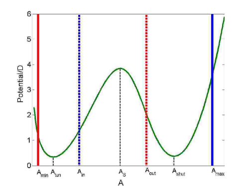
Figure 7.14: Bistable effective potential for the SDQS coexistence regime. The important amplitudes for the calculation of the rates are indicated. The reflecting (full) and absorbing (dashed) borders for the calculation of the escape rates.

We define the probability density $P(x,t|A_{\rm tun},0)$ for the stochastic variable $A(t)$ starting at $t=0$ with $A(0)=A_{\rm tun}$ to be in $x$ at time $t$ without reaching the upper border $A_{\rm out}$. It is possible to demonstrate [50] that the probability $P$ must obey the Kramers equation (7.110) if $A_{\rm min}<x<A_{\rm out}$, is identically zero for $x\geq A_{\rm out}$ since the walks that touch the upper border are not taken into account and satisfy reflecting boundary conditions at the lower border, namely:

$$\begin{split}&\frac{\partial P}{\partial t}=\mathcal{L}_{K}P;\quad P(x,0|A_{\rm tun},0)=\delta(x-A_{\rm tun})\quad\textrm{for}\quad A_{\rm min}<x<A_{\rm out}\\ &P(x,t|A_{\rm tun},0)=0\quad\textrm{for}\quad x=A_{\rm out}\\ &\partial_{x}e^{\frac{\mathcal{V}(x)}{D}}P(x,t|A_{\rm tun},0)|_{x=A_{\rm min}}=0\end{split}$$ (7.130)

where $\mathcal{L}_{K}$ is the Kramers’ Liouvillean of equation (7.110). The probability $W(A_{\rm tun},t)$ of realizations which have started at $A_{\rm tun}$ and which have not yet reached the upper boundary up to the time $t$ is given by:

$$W(A_{\rm tun},t)=\int_{A_{\rm min}}^{A_{\rm out}}P(x,t|A_{\rm tun},0)dx$$ (7.131)

The probability $-dW$ of those realizations which reach the upper boundary in the time interval $(t,t+dt)$ thus reads

$$-dW(A_{\rm tun},t)=-\int_{A_{\rm min}}^{A_{\rm out}}\dot{P}(x,t|A_{\rm tun},0)dxdt$$ (7.132)

The distribution $w(T)$ function for the first passage time T is therefore given by

$$w(A_{\rm tun},T)=-\frac{dW(A_{\rm tun},T)}{dT}=-\int_{A_{\rm min}}^{A_{\rm out}}\dot{P}(x,T|A_{\rm tun},0)dx$$ (7.133)

The moments of the first-passage time distribution are

$$T_{n}(A_{\rm tun})=\int_{0}^{\infty}T^{n}w(A_{\rm tun},T)dT=\int_{A_{\rm min}}^{A_{\rm out}}p_{n}(x,A_{\rm tun})dx$$ (7.134)

where $p_{n}(x,A_{\rm tun})$ is defined by

$$p_{n}(x,A_{\rm tun})=-\int_{0}^{\infty}T^{n}\dot{P}(x,T|A_{\rm tun},0)dT$$ (7.135)

We obviously have

$$p_{0}(x,A_{\rm tun})=-\int_{0}^{\infty}\dot{P}(x,T|A_{\rm tun},0)dT=P(x,0|A_{\rm tun},0)=\delta(x-A_{\rm tun})$$ (7.136)

Performing a partial integration gives the relation

$$p_{n}(x,A_{\rm tun})=n\int_{0}^{\infty}T^{n-1}P(x,T|A_{\rm tun},0)dT$$ (7.137)

Applying the Kramers’ Liouvillean $\mathcal{L}_{K}$ to equation (7.137) we obtain the recursive relation:

$$\mathcal{L}_{K}[p_{n}(x,A_{\rm tun})]=-np_{n-1}(x,A_{\rm tun})$$ (7.138)

and in particular

$$\mathcal{L}_{K}[p_{1}(x,A_{\rm tun})]=-\delta(x-A_{\rm tun})$$ (7.139)

In other words the function $p_{1}(x,A_{\rm tun})$ that enters the definition of the average first-passage time is the Green’s function of the Kramers’ Liouvillean $\mathcal{L}_{K}$. The Kramers’ Liouvillean can be written in the form:

$$\mathcal{L}_{K}=D\partial_{A}e^{-\frac{\mathcal{V}(A)}{D}}\partial_{A}e^{+\frac{\mathcal{V}(A)}{D}}$$ (7.140)

as can be easily proven by acting with the last partial derivative on the exponential. It is also possible to give an analytic expression for the Green’s function $p_{1}(x,A_{\rm tun})$ of the Kramers’ Liouvillean $\mathcal{L}_{K}$:

$$p_{1}(A,A_{\rm tun})=\frac{1}{D}e^{-\frac{\mathcal{V}(A)}{D}}\int_{A}^{A_{\rm out}}e^{\frac{\mathcal{V}(B)}{D}}\left[\int_{A}^{A_{\rm out}}\delta(C-A_{\rm tun})dC\right]dB$$ (7.141)

The mean-escape time from the tunneling well reads:

$$T_{1}(A_{\rm tun})=\frac{1}{D}\int_{A_{\rm min}}^{A_{\rm out}}\left\{e^{-\frac{\mathcal{V}(A)}{D}}\int_{A}^{A_{\rm out}}e^{\frac{\mathcal{V}(B)}{D}}\left[\int_{A_{\rm min}}^{B}\delta(C-A_{\rm tun})dC\right]dB\right\}dA$$ (7.142)

The escape time from the shuttling well can be calculated exactly in the same way using $A_{\rm shut}$ as starting point for the random process and $A_{\rm in}$ and $A_{\rm max}$ as boundaries (see Fig. 7.14). The calculation of the integrals in (7.142) can be simplified considering that the integrand has a sharp maximum in the region $(A,B)\approx(A_{\rm tun},A_{\rm S})$ due to the behaviour of the effective potential $\mathcal{V}$ around those two points. The escape time from the shuttling well can be calculated in a similar way. We obtain in the end the switching rates:

$$\begin{split}\Gamma_{\rm out}&=D\left(\int_{A_{\rm tun}}^{A_{\rm out}}dB\,e^{\frac{{\mathcal{V}}(B)}{D}}\int_{A_{\rm min}}^{B}dA\,e^{-\frac{{\mathcal{V}}(A)}{D}}\right)^{-1}\\ \Gamma_{\rm in}&=D\left(\int_{A_{\rm in}}^{A_{\rm shut}}dB\,e^{\frac{{\mathcal{V}}(B)}{D}}\int_{B}^{A_{\rm max}}dA\,e^{-\frac{{\mathcal{V}}(A)}{D}}\right)^{-1}\\ \end{split}$$ (7.143)

We recall here the equation for the current and the Fano factor for a dichotomous process inserting now the particular currents and switching rates characteristic of the SDQS coexistence regime:

$$\begin{split}I^{\rm stat}&=\frac{I_{\rm sh}\Gamma_{\rm out}+I_{\rm tun}\Gamma_{\rm in}}{\Gamma_{\rm in}+\Gamma_{\rm out}}\\ F&=\frac{S(0)}{I^{\rm stat}}=2\frac{(I_{\rm sh}-I_{\rm tun})^{2}}{I_{\rm sh}\Gamma_{\rm out}+I_{\rm tun}\Gamma_{\rm in}}\frac{\Gamma_{\rm in}\Gamma_{\rm out}}{(\Gamma_{\rm in}+\Gamma_{\rm out})^{2}}\end{split}$$ (7.144)

They represent, together with the stationary distribution

$$\mathcal{W^{\rm stat}}(A)=\frac{1}{\mathcal{Z}}\exp\left(-\frac{\mathcal{V}(A)}{D}\right)$$ (7.145)

the starting point for a quantitative comparison between the simplified model and the full description.

7.3.4 Comparison

The classical (but “noisy”) limit

The comparison between the dichotomous process model and the full description for the coexistence regime is based, as for the other regimes, on the three investigation tools: phase-space distribution, current and current-noise.

The phase space distribution is the most sensitive method to compare the model and the full description. One of the basic procedures adopted in the derivation of the Kramers equation (7.110) is the expansion to second order in the small parameters (7.96). In order to test the reliability of the model we simplify as much as possible the description reducing the model to a classical description: namely taking the zero limit for the parameter $\left(\frac{x_{0}}{\lambda}\right)$. We realize physically this condition assuming a large temperature and a tunneling length $\lambda$ of the order of the thermal length $\lambda_{\rm th}=\sqrt{\frac{k_{B}T}{m\omega^{2}}}$. We partially discussed this limit in the previous chapters. Also the full description is slightly changed, but not qualitatively: the three regimes are still clearly present with their characteristics. The numerical calculation is though based on a totally different approach.

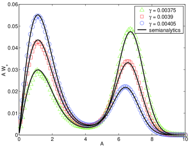
Figure 7.15: Stationary amplitude probability distribution $\mathcal{W}$ for the SDQS in the coexistence regime. We compare the results obtained from the simplified model (full line) and from the full description (circles, triangles and squares). These results are obtained in the classical high temperature regime $k_{B}T\gg\hbar\omega$. The amplitude is measured in units of $\lambda_{\rm th}=\sqrt{\frac{k_{B}T}{m\omega^{2}}}$. The mechanical damping $\gamma$ in units of the mechanical frequency $\omega$. The other parameter values are $d=0.05\lambda_{\rm th}$ and $\Gamma=0.015\omega$, $\lambda=2\lambda_{\rm th}$.

In figures 7.15, 7.16 and 7.17 we present respectively the results for the stationary Wigner function, the current and the Fano factor in the semiclassical approximation and full description.

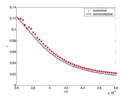
Figure 7.16: Current in the coexistence regime of SDQS. Comparison between semianalytical and full numerical description. For the parameter values see Fig. 7.15.

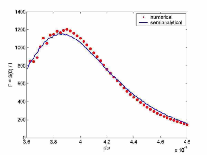
Figure 7.17: Fano factor in the coexistence regime of SDQS. Comparison between semianalytical and full numerical description. For the parameter values see Fig. 7.15.

The quantum limit

The coexistence regime in the parameters corner typically presented in this thesis (e.g. Fig. 5.5) is not captured by the model we introduced. The concept of elimination of the fast dynamics is still correct, but the small parameters expansion fails. The effective potential calculated from a second order expansion still gives the position of the ring structure with reasonable accuracy but the overall stationary Wigner function is not reproduced due to a non convergent diffusion function $D(A)$. It is clear that we need to consider higher order terms in the parameter $(x_{0}/\lambda)^{2}$. This represents nevertheless a fundamental problem since it would produce terms with higher order derivatives with respect to the amplitude $A$ in the Fokker-Planck equation and consequently, to our knowledge, the break down of the escape time theory.

It has nevertheless been demonstrated with the help of the higher cumulants of the current that the dichotomous process description of the coexistence regime is valid also more in the quantum regime ($\lambda=1.5x_{0}$), the only necessary condition being a separation of the ring and dot structures in the stationary Wigner function distribution [51].

Motivated by the fact that the effective potential was able to give the correct position of the shuttling ring we used the diffusion constant as a fitting parameter. The current and the Fano factor are very nicely reproduced in terms of a fitted diffusion constant approximately doubled with respect to the one calculated at zero temperature with no $\left(\frac{x_{0}}{\lambda}\right)^{4}$ corrections (Figs. 7.18 and 7.19).

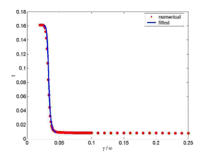
Figure 7.18: Current in the coexistence regime of SDQS. Comparison between semianalytical description with an effective fitted diffusion constant (see the text for explanation) and full numerical description. The parameter values are $\Gamma=0.01\omega$, $\lambda=2x_{0}$, $d=0.5x_{0}$, $T=0$.

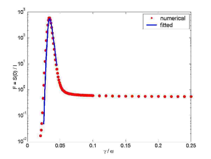
Figure 7.19: Fano factor in the coexistence regime of SDQS. Comparison between semianalytical description with an effective fitted diffusion constant (see the text for explanation) and full numerical description. The parameter values are $\Gamma=0.01\omega$, $\lambda=2x_{0}$, $d=0.5x_{0}$, $T=0$.

The full numerical description presented in this thesis is relatively fragile with respect to the modification of the tunneling length at least for two reasons: the enlargement of the shuttling amplitude enlarges the number of oscillator states relevant for the dynamics to untractable numbers; the preconditioning loses effectiveness and the problem is not convergent. For this reason we are (still) lacking a numerical benchmark for the intermediate range of values of the tunneling length $\lambda>x_{0}$ but which is still non-classical where a second order expansion in the small parameter $\left(\frac{x_{0}}{\lambda}\right)^{2}$ is probably a good approximation.

Chapter 8 Conclusions

We summarize in this chapter the main results presented in the thesis. The richness of the shuttle model still leaves many points open in the description and understanding of the device dynamics. We close the chapter listing some of the open questions that could encourage a continuation of the present work.

8.1 Summary

We analyzed in this thesis the dynamics of two different shuttle devices: the single- and the triple-dot quantum shuttles. Shuttle devices are nanoelectromechanical systems (NEMS) in which an oscillating quantum dot can transfer electrons one per cycle from source to drain lead. The dynamics of such devices is the result of a strong interplay between their mechanical and electrical degrees of freedom.

The electrical dynamics is permeated of quantum effects: electrons can go from the source to the quantum dot and finally to the drain lead only via tunneling events; the small capacitance of the oscillating dot and the corresponding large charging energy reveals the discrete nature of the electrical charge; finally the presence of three coupled quantum dots is also a source of coherent electrical dynamics in the TDQS. The small size of the device makes quantum effects important also for the mechanical degree of freedom. The resonance frequency in such small (and relatively stiff) devices can be in the order of GHz. Consequently the quantum of energy of the harmonic oscillator is comparable with other energies in the device.

For these reasons for the SDQS we developed quantum models: we extended for the SDQS the classical model proposed by Gorelik et al. [1] and we adopted for the TDQS the one already existing invented by A. Armour and A. MacKinnon [7].

Among the different approaches for the description of the dynamics of a quantum system we chose the Generalized Master Equation (GME). GME’s are particularly well-suited to study small open quantum systems (i.e. systems with a small number of degrees of freedom in contact with resevoirs but still conserving some coherent dynamics) since they neglect the many (irrelevant) degrees of freedom of the resevoirs still keeping track of the residual quantum coherencies of the small system.

The shuttle devices are small quantum systems in contact with two kinds of resevoirs: the leads and the thermal bath. The strength of the coupling is very different and calls for a different treatment. The weak coupling between the thermal bath and the mechanical degree of freedom of the device justifies the perturbation theory and the quantum-optical derivation of a GME in Born-Markov approximation. The tunneling coupling of the shuttling devices to their electrical baths (the leads) is not weak. It sets, on the contrary, the time scale of the electrical dynamics that in the shuttling regime is comparable with the period of the mechanical oscillations in the system. This strong coupling condition is realized by a tunneling amplitude modulated by the displacement of the quantum dot from the equilibrium position in the SDQS while is directly set by a model parameter in the TDQS. In order to handle the strong coupling we adopted the Gurvitz method for the derivation of the GME and extended the original formulation to take into account the mechanical degree of freedom.

The shuttle dynamics has, especially in the single dot device, an appealing simple classical interpretation and one can say that the name itself of “shuttle” suggests the idea of sequential and periodical loading, mechanical transport and unloading of electrons between a source and a drain lead. For this reason, while preserving the complete quantum treatment that we achieved with the GME, we wanted to keep as much as possible the intuitive classical picture and the possibility to handle the quantum-classical correspondence. The Wigner function distribution seemed to us a good answer to all these requirements. It allows a clear visualization of the numerical results obtained within the framework of the GME and it shows in its equation of motion (the Klein-Kramers equation) an explicit quantum-classical correspondence (expansion in powers of $\hbar$) [34].

Having the methods for the analysis of the shuttle device dynamics we looked for investigation tools. We first realized that a clear finger-print of the shuttling regime that distinguishes it from other kinds of phonon assisted tunneling is the charge-position(momentum) correlation. The Wigner distribution function on the device phase space (i.e. also charge resolved to take into account the two electrical states of the quantum dot) is a perfect tool to visualize this property. The only problem with the Wigner distribution functions is that it seems very difficult (if not impossible) to access experimentally these functions. For this reason, with the guidance of the distribution function description, we investigated the electronic transport properties in the shuttle devices (more realistically measurable): first the stationary current and then the current-noise. A special rôle in the calculation of the current-noise for the SDQS was played by a specific characteristic of the GME obtained in the Gurvitz approach. In this method the information on the state of the leads in not completely traced out and the number $n$ of electrons that passed through the device after a specific time appears in the equation of motion for the so-called $n$-resolved reduced density matrix.

With these tools we investigated the properties of the quantum shuttle devices. The sharp tunneling-shuttling transition found by Gorelik et al. for the semiclassical model turned into a smooth crossover. We also could recognize the onset of the shuttling regime triggered by quantum mechanical noise with no external electric field acting on the oscillating quantum dot. The shuttle regime also revealed the characteristic current quantization (in our set-up a saturation due to Coulomb blockade to one electron per cycle in the cleanest shuttling regime) and the extremely low noise typical of a quasi-deterministic transport regime. With all the three investigation tools we adopted we could recognize three operating regimes for the shuttle device: tunneling, shuttling and coexistence regime. They represent for the SDQS the whole scenario of possible dynamics. Part of the complexity of the TDQS is also captured in this scheme.

The specific separation of time scales in the different regimes allowed us to identify the relevant variables and describe each regime by a specific simplified model. In the tunneling (high damping) regime the mechanical degree of freedom is almost frozen and all the features revealed by the Wigner distribution, the current and the current noise can be reproduced with a resonant tunneling model with tunneling rates renormalized due to the movable quantum dot. Most of the features of the shuttling regime (self-sustained oscillations, charge-position correlation and current quantization) are captured by a simple model derived as the zero-noise limit of the full description. Finally for the coexistence regime we proposed a dynamical picture in terms of slow dichotomous switching between the tunneling and shuttling modes. This interpretation was mostly suggested by the presence in the stationary Wigner function distributions of both the characteristic features of the tunneling and shuttling dynamics and by a corresponding gigantic peak in the Fano factor. We based the derivation of the simplified model on the fast variables elimination from the Klein-Kramers equations for the Wigner function and a consequent derivation of an effective bistable potential for the amplitude of the dot oscillation (the relevant slow variable in this regime).

8.2 Some open questions

During the developing of the present work many questions arose about possible phenomena to investigate in different shuttle devices or other possible regimes that the systems we investigate could exhibit in some other parameter corner that we did not reach. This questions could be of interest for example in understanding or proposing future experiments. We list them here as a spur for possible continuation of the present work sure that some of the theoretical tools presented in this thesis are definitely useful for those tasks.

• The mechanical bath introduces decoherence in the mechanical degree of freedom, the leads in the electrical. Correlations are left (in the SDQS) only in the off-diagonal elements of the charge resolved density matrices. Can we imagine an electromechanical system that instead exhibits quantum coherence in the mechanical degree of freedom? Could we use the electromechanical interaction to “pump” continuously coherence in the device?

• The stationary solution for the GME is incoherent. Is there any possibility to reduce the GME to an effective Master equation? We imagine that especially in the coexistence regime this could help to avoid the Wigner function small parameter expansion for the calculation of the effective bistable potential and lead directly to the calculation of the rates for the slow switching process. This would make the calculation of the parameters for the dichotomous process description much more general.

• Taking into account the spin degrees of freedom and the Coulomb blockade the incoming bare rate should be considered as double with respect to the out going rate. This fact does not change qualitatively the picture since the switching is, in first approximation a non-dissipative process and the electrostatic force is a small perturbation of the oscillator restoring force. The mechanical trajectories are not significantly changed (maybe slightly decreased in radius) and only the symmetry between the two charged resolved Wigner functions is modified in favour of $W_{11}$: the dot is charged for a longer time. But what happens if we consider a spin dynamics on the dot due for example to a coupling to an external magnetic field?

• At high bare injection rates ($\Gamma\gg\omega$) the shuttle device is more stable and hardly leaves the tunneling regime. The mechanical motion cannot in fact follow the fast electrical forcing and the effect is generally uncorrelated resonant tunneling. Nevertheless at extremely low damping the shuttling regime arises. The transition is very different from the small injection rate shuttling instability: it is very smooth and the ring structure gradually emerges from the central fuzzy spot typical for the tunneling regime. The general question is: can we draw a phase diagram for shuttling devices as a function of their parameters?

• A big issue regards the treatment of the bias in the quantum description. All our equations were derived in the limit of high external bias. We did not have access to this parameter and we used for this reason the mechanical damping as a control parameter. Is it possible to derive a GME at low bias and for strong couplings to the leads? Probably the dynamics will get non-Markovian and all kinds of coherent transport effects will also enter the game. We know from the semiclassical treatment that the shuttling instability should be present. Can we understand something new from the quantum treatment?

Bibliography

- [1] L. Y. Gorelik, A. Isacsson, M. V. Voinova, B. Kasemo, R. I. Shekhter, and M. Jonson, Shuttle Mechanism for Charge Transfer in Coulomb Blockade Nanostructures, Phys. Rev. Lett. 80(20), 4526 (May 1998).
- [2] A. Isacsson, L. Y. Gorelik, M. V. Voinova, B. Kasemo, R. I. Shekhter, and M. Jonson, Shuttle instability in self-assembled Coulomb blockade nanostructures, Physica B 255, 150–163 (December 1998).
- [3] C. Weiss and W. Zwerger, Accuracy of a mechanical single-electron shuttle, Europhys. Lett. 47(1), 97–103 (July 1999).
- [4] N. Nishiguchi, Gate voltage dependence of a single-electron transistor using the shuttle mechanism, Phys. Rev. B 65(3), 035403 (December 2001).
- [5] F. Pistolesi, Full counting statistics of a charge shuttle, Phys. Rev. B 69(24), 245409 (June 2004).
- [6] T. Nord and A. Isacsson, Impact of van der Waals forces on the classical shuttle instability, Phys. Rev. B 69(3), 35309 (January 2004).
- [7] A. D. Armour and A. MacKinnon, Transport via a quantum shuttle, Phys. Rev. B 66(3), 035333 (July 2002).
- [8] T. Novotný, A. Donarini, and A.-P. Jauho, Quantum Shuttle in Phase Space, Phys. Rev. Lett. 90(25), 256801 (June 2003).
- [9] D. Fedorets, L. Y. Gorelik, R. I. Shekhter, and M. Jonson, Quantum Shuttle Phenomena in a Nanoelectromechanical Single-Electron Transistor, Phys. Rev. Lett. 92(16), 166801 (April 2004).
- [10] A. Donarini and A.-P. Jauho, Shuttle instabilities: semiclassical phase analysis, Physica E 22(1–3), 721 (April 2004).
- [11] A. Donarini, T. Novotný, and A.-P. Jauho, Quantum theory of shuttling instability in a movable quantum dot array, Semicond. Sci. Technol. 19(4), S430 (April 2004).
- [12] C. Flindt, Current Noise in a 3-Dot Quantum Shuttle, Master’s thesis, MIC, Technical University of Denmark, March 2004.
- [13] A. Romito, F. Plastina, and R. Fazio, Decoherence in a Cooper pair shuttle, Phys. Rev. B 68(14), 140502 (October 2003).
- [14] A. Romito and Y. V. Nazarov, Full Counting Statistics of Cooper Pair Shuttling, cond-mat/0402412, February 2004.
- [15] L. Y. Gorelik, A. Isacsson, Y. M. Galperin, R. I. Shekhter, and M. Jonson, Coherent transfer of Cooper pairs by a movable grain, Nature 411, 454 (May 2001).
- [16] L. Y. Gorelik, R. I. Shekhter, M. Jonson, S. I. Kulinich, and V. M. Vinokur, Spin-Dependent Transport of Electrons in a Shuttle Structure, cond-mat/0402284, February 2004.
- [17] A. Erbe, C. Weiss, W. Zwerger, and R. H. Blick, Nanomechanical Resonator Shuttling Single Electrons at Radio Frequencies, Phys. Rev. Lett. 87(9), 096106 (August 2001).
- [18] H. Park, J. Park, A. K. L. Lim, E. H. Anderson, A. P. Alivisatos, and P. L. McEuen, Nanomechanical oscillations in a single-C60 transistor, Nature 407, 57 (September 2000).
- [19] D. Fedorets, L. Y. Gorelik, R. I. Shekhter, and M. Jonson, Vibrational instability due to coherent tunneling of electrons, Europhys. Lett. 58(1), 99–104 (April 2002).
- [20] D. Boese and H. Schoeller, Influence of nanomechanical properties on single-electron tunneling: A vibrating single-electron transistor, Europhys. Lett. 54(5), 668–674 (June 2001).
- [21] K. D. McCarthy, N. Prokof’ev, and M. T. Tuominen, Incoherent dynamics of vibrating single-molecule transistors, Phys. Rev. B 67(24), 245415 (June 2003).
- [22] T. Brandes and N. Lambert, Steering of a bosonic mode with a double quantum dot, Phys. Rev. B 67(12), 125323 (March 2003).
- [23] T. Novotný, A. Donarini, C. Flindt, and A.-P. Jauho, Shot Noise of a Quantum Shuttle, Phys. Rev. Lett. 92(24), 248302 (June 2004).
- [24] D. V. Scheible and R. Blick, Silicon nanopillars for mechanical single-electron transport, Appl. Phys. Lett. 84(23), 4632 (June 2004).
- [25] E. Onofri and C. Destri, Istituzioni di Fisica Teorica, Carocci, first edition, 1998.
- [26] K. Huang, Statistical Mechanics, John Wiley & Sons, second edition, 1987.
- [27] C. W. Gardiner and P. Zoller, Quantum Noise, Springer, second edition, 2000.
- [28] S. A. Gurvitz and Y. S. Prager, Microscopic derivation of rate equations for quantum transport, Phys. Rev. B 53(23), 15932–15942 (June 1996).
- [29] M. R. Wegewijs and Y. V. Nazarov, Resonant tunneling through linear arrays of quantum dots, Phys. Rev. B 60(20), 14318 (November 1999).
- [30] D. Kohen, C. C. Marston, and D. J. Tannor, Phase space approach to theories of quantum dissipation, J. Chem. Phys. 107(13), 5236 (October 1997).
- [31] T. Eirola and O. Nevanlinna, Numerical linear algebra; iterative methods, Lecture notes, Helsinki University of Technology, 2003.
- [32] G. H. Golub and C. F. V. Loan, Matrix Computations, The John Hopkins University Press, third edition, 1996.
- [33] C. Flindt, T. Novotný, and A.-P. Jauho, Current noise in a vibrating quantum dot array, cond-mat/0405512, May 2004, accepted to PRB.
- [34] M. Hillery, R. F. O’Connell, M. O. Scully, and E. P. Wigner, Distribution functions in physics: fundamentals, Phys. Rep. 106(3), 121 (1984).
- [35] R. F. O’Connell and E. P. Wigner, Quantum-mechanical distribution functions: conditions for uniqueness, Phys. Lett. A 83A(4), 145 (1981).
- [36] S. Braig and K. Flensberg, Vibrational sidebands and dissipative tunneling in molecular transistors, Phys. Rev. B 68(20), 205324 (November 2003).
- [37] Y. M. Blanter and M. Büttiker, Shot noise in mesoscopic conductors, Physics Reports 336(1–2), 1–166 (September 2000).
- [38] C. Beenakker and C. Schönenberger, Quantum Shot Noise, Physics Today 56(5), 37 (May 2003).
- [39] A. Mitra, I. Aleiner, and A. J. Millis, Phonon effects in molecular transistors: Quantual and classical treatment, Phys. Rev. B 69(24), 245302 (June 2004).
- [40] A. D. Armour, M. P. Blencowe, and Y. Zhang, Classical dynamics of a nano-mechanical resonator coupled to a single-electron transistor, Phys. Rev. B 69, 125313 (March 2004).
- [41] N. M. Chtchelkatchev, W. Belzig, and C. Bruder, Charge transport through a SET with a mechanically oscillating island, cond-mat/0401486, January 2004.
- [42] A. Isacsson and T. Nord, Low-frequency current noise of the single-electron shuttle, Europhys. Lett. 66(5), 708 (June 2004).
- [43] B. Elattari and S. A. Gurvitz, Shot noise in coupled dots and the “fractional charges”, Phys. Lett. A 292, 289 (January 2002).
- [44] H. Bruus and K. Flensberg, Many-Body Quantum Theory in Condensed Matter Physics, Oxford University Press, Oxford, 2003.
- [45] J. H. Davies, P. Hyldgaard, S. Hershfield, and J. W. Wilkins, Classical theory of shot noise in resonant tunneling, Phys. Rev. B 46(15), 9620 (October 1992).
- [46] H.-P. Breuer and F. Petruccione, The Theory of Open Quantum Systems, Oxford University Press, first edition, 2002.
- [47] D. Fedorets, L. Y. Gorelik, R. I. Shekhter, and M. Jonson, Spintronics of a Nanoelectromechanical Shuttle, cond-mat/0408591, August 2004.
- [48] T. Naeh, M. M. Klosek, B. J. Matkowsky, and Z. Schuss, A direct approach to the exit problem, SIAM J. Appl. Math. 50(2), 595 (April 1990).
- [49] D. Ludwig, Persistence of dynamical systems under random perturbations, SIAM Review 17(4), 605 (October 1975).
- [50] H. Risken, The Fokker-Planck Equation, Springer, Berlin, 1996.
- [51] C. Flindt, T. Novotný, and A.-P. Jauho, Full counting statistics of nano-electromechanical systems, cond-mat/0410322, October 2004.