The square-lattice $F$ model revisited: a loop-cluster update scaling study

Abstract

The six-vertex $F$ model on the square lattice constitutes the unique example of an exactly solved model exhibiting an infinite-order phase transition of the Kosterlitz-Thouless type. As one of the few non-trivial exactly solved models, it provides a welcome gauge for new numerical simulation methods and scaling techniques. In view of the notorious problems of clearly resolving the Kosterlitz-Thouless scenario in the two-dimensional XY model numerically, the $F$ model in particular constitutes an instructive reference case for the simulational description of this type of phase transition. We present a loop-cluster update Monte Carlo study of the square-lattice $F$ model, with a focus on the properties not exactly known such as the polarizability or the scaling dimension in the critical phase. For the analysis of the simulation data, finite-size scaling is explicitly derived from the exact solution and plausible assumptions. Guided by the available exact results, the careful inclusion of correction terms in the scaling formulae allows for a reliable determination of the asymptotic behaviour.

,

1 Introduction

An ice-type or vertex model was first proposed by Pauling pauling:35a as a model for (type I) water ice. It was known that ice forms a hydrogen-bonded crystal, i.e., the oxygen atoms are located on a four-valent lattice and the bonding is mediated by one hydrogen atom per bond. Pauling proposed that there be some non-periodicity in the arrangement of the hydrogen bonds in that the hydrogen atoms could be located nearer to one or the other end of the bond. This positioning should satisfy the ice rule, stating that always two of the bonds are in the “close” position and two are in the “remote” position with respect to the considered oxygen atom. Denoting the position of the hydrogen atom by a decoration of the bond with an arrow pointing to the closer oxygen, this leads to the arrow configurations depicted in figure 1 when for simplicity placing the oxygens on a square lattice instead of the physically realized diamond lattice. Generalizing the resulting six-vertex model for square ice, one assigns energies $\epsilon_{i}$, $i=1,\ldots,6$, to the vertex configurations depicted in figure 1, resulting in Boltzmann factors $\omega_{i}=\exp(-\beta\epsilon_{i})$, where $\beta=1/k_{B}T$ is the inverse temperature or coupling. Assuming an overall arrow reversal symmetry (corresponding to the absence of an external electric field), one abbreviates $a=\omega_{1}=\omega_{2}$, $b=\omega_{3}=\omega_{4}$ and $c=\omega_{5}=\omega_{6}$. Then, the original ice model corresponds to the choice $\epsilon_{i}=0$, $i=1,\ldots,6$, whereas another especially symmetric version assumes

$$\epsilon_{a}=\epsilon_{b}=1,\;\;\epsilon_{c}=0\;\;\;\mathrm{resp.}\;\;\;a=b=e^{-\beta},\;\;c=1,$$ (1)

which is known as the $F$ model of anti-ferroelectrics rys:63a , since due to the choice of weights the vertex configurations 5 and 6 will dominate for low temperatures, resulting in a ground-state of staggered, anti-ferroelectric order as depicted in figure 2.

The six-vertex model as well as the more general eight-vertex models, obtained by including sink and source vertices with all four arrows pointing in and out, respectively, have been exactly solved in zero field using transfer matrix techniques, see reference baxter:book . They exhibit rich phase diagrams featuring first-order and continuous phase transitions as well as multi-critical points. In particular, the six-vertex $F$ model undergoes an infinite-order transition of the Berezinskii-Kosterlitz-Thouless (BKT) type to an anti-ferroelectrically ordered phase and the scaling behaviour of the basic thermodynamic quantities can be extracted from the closed-form solution. Since there is no solution of the model in a (staggered) field, however, information about properties related to the polarization is incomplete. The same is true for the correlation function, which can only be evaluated at the so-called free-fermion point of the model baxter:70a , baxter:book (the correlation length, however, is exactly known for all temperatures, see below). Also, since the solution was obtained in the thermodynamic limit, information about finite-size scaling (FSS) is not exact, but must be deduced from scaling arguments. Apart from its prominent position as a non-trivial solvable model of statistical mechanics, the $F$ model has enjoyed sustained interest due to its equivalence to the BCSOS surface model beijeren:77a , and hence several dynamical generalizations of the six-vertex model have been considered levi:97a . A six-vertex model with so-called domain-wall boundary conditions has recently attracted considerable interest and found numerous applications in counting problems, the quantum inverse scattering method etc. bogoliubov:02a .

Figure 1: Allowed arrow configurations for the six-vertex model on the square lattice, restricted by the ice rule.

The Berezinskii-Kosterlitz-Thouless bkt scenario of an infinite-order phase transition induced by the unbinding of vortex pairs in the two-dimensional XY model has been found exceptionally hard to confirm numerically guptaetal , wj:93a , kenna:97a , wj:97b . This is partially due to the nature of the infinite-order phase transition itself, which is not easy to distinguish from a finite-order transition numerically, and the presence of a critical phase, which render many of the standard FSS techniques less useful. The main trouble, however, is caused by the presence of logarithmic corrections, expected to be present on general grounds for a theory with central charge $c=1$ henkel:book and explicitly found from the BKT theory of the model amitkadanoff . While a numerical confirmation of the leading scaling behaviour of the BKT transition has been achieved in the past decade or so, the resolution of the logarithmic scaling corrections is still at the forefront of problems amenable to numerical investigation today wj:97a , balog:01a , hasenbusch:05a .

Figure 2: Cutout of one of the two anti-ferroelectrically ordered ground states of the square-lattice $F$ model. The state consists of vertices $5$ and $6$ at equal proportions. The dashed lines indicate one of two tilted sub-lattices of ferroelectrical order.

From duality arguments and mapping to Coulomb gas systems, the $F$ model is known to be asymptotically equivalent to the two-dimensional XY model at criticality. Thus, apart from being an interesting subject in its own right, a detailed analysis of the thermal and FSS properties of the six-vertex $F$ model in the critical phase and at its BKT point serves as a guideline for simulations of the XY model case. Guidance is been given here through the fact that the exact solution of the $F$ model yields the leading singularities including the correction terms explicitly, and, most notably for numerical purposes, the exact critical coupling of the model. Uncertainties occurring in analyses of the XY model such as systematic errors in the determination of the transition point or the effect of neglected higher-order correction terms can be studied rather explicitly for the $F$ model. Finally, when it is found here that one has to consider large system sizes and proceed carefully when including correction terms into the fits, this situation should also be put into relation with the case of an $F$ model placed on an annealed ensemble of random lattices considered recently weigel:04b . Guided by the present investigation, this case has to be analyzed even more carefully due to an additional fractality of the lattices, which reduces the effective linear extent of the amenable lattice sizes, thus increasing finite-size effects even further.

The other paradigm example of an exactly solved non-trivial model of statistical mechanics, the two-dimensional Ising model, has served as a benchmark system and playground for new ideas in the theory of critical phenomena as well as for new algorithms in computer simulations in an overwhelming number of studies, and almost all of its aspects have been investigated (but not necessarily understood). In contrast, for the case of vertex models only rather recently efficient cluster-update Monte Carlo algorithms have been developed evertz:loop , barkema:98a , syljuasen:04a , mainly with the mapping of vertex models on quantum chains in mind, and some simulations of special aspects of the six-vertex model, such as dynamical critical exponents of the considered algorithms evertz:93b , barkema:98a , properties of the equivalent surface models mazzeo , matching of renormalization-group flows with the XY model hasenbuschpinn , or the case of domain-wall boundary conditions syljuasen:04a have been analyzed. A systematic thermal and FSS study of the $F$ model in the critical high-temperature phase, at the critical point and its low-temperature vicinity including the analysis of the logarithmic correction terms, however, is to our best knowledge lacking so far.

The rest of the paper is organized as follows. In section 2 we outline the extent of exact knowledge about the phase diagram and the occurring transitions of the six-vertex model and the $F$ model in particular and give an overview over scaling at a BKT point in general. After a short description of the simulational setup used, section 3 contains a report of the analysis of the simulation data, comprising the FSS analyses of the critical-point thermodynamic properties (where the corresponding FSS relations are explicitly derived from the closed-form solution), an investigation of the behaviour in the critical phase as well as a thermal scaling analysis in the low-temperature phase of the model. Finally, section 4 contains our conclusions.

2 Analytical Results

2.1 Exact solution and phase diagram

The square-lattice, zero-field six-vertex model has been solved exactly in the thermodynamic limit by means of the Bethe ansatz by Lieb lieb and Sutherland sutherland:67a . The analytic structure of the free energy is most conveniently parametrized in terms of the reduced coupling

$$\Delta=\frac{a^{2}+b^{2}-c^{2}}{2ab},$$ (2)

such that the free energy takes a different analytic form depending on whether $\Delta<-1$, $-1<\Delta<1$ or $\Delta>1$. This leads to a phase diagram of the model consisting of four distinct phases as shown in figure 3. The phases I and II are both characterized by $\Delta>1$, thus corresponding to the same analytic form of the free energy; they represent ferroelectrically ordered phases, the ground-states being related to each other through a global rotation by $\pi/2$. In these phases, the system exhibits the peculiarity of sticking to the respective ground-states also for non-zero temperatures. The intermediate case $-1<\Delta<1$, corresponding to phase III, includes the infinite temperature point $a=b=c=1$ and thus belongs to a disordered phase, which turns out to be massless, i.e., it exhibits algebraic correlations throughout. This latter effect can be traced back to the fact that the six-vertex model corresponds to a critical surface in the phase diagram of the eight-vertex model. Finally, for $\Delta<-1$ one has $c>a+b$, resulting in the anti-ferroelectric order of phase IV described above for the $F$ model. The parameter space of the $F$ model is restricted to the dashed line connecting phases III and IV indicated in figure 3. The dotted line of figure 3 indicates the curve $\Delta=0$, where the six-vertex model is equivalent to a system of free fermions and an exact solution is even possible in the presence of a staggered field baxter:70a , baxter:book . The nature of the transitions between the phases I–IV can be extracted from the exact solution lieb , sutherland:67a , baxter:book . Crossing the phase boundaries I $\rightarrow$ III and II $\rightarrow$ III one finds discontinuities corresponding to first-order transitions. The transition III $\rightarrow$ IV, on the other hand, is peculiar in that all the temperature derivatives of the free energy exist and vanish exponentially as the transition is approached. These are the properties of a BKT phase transition to be detailed below in section 2.2.

While the ferroelectrically ordered phases I and II exhibit a plain polarization, which can be used as an order parameter for the corresponding transition, the anti-ferroelectric order of phase IV is accompanied by a staggered polarization with respect to a sub-lattice decomposition of the square lattice. This is equivalent to a mutually inverse plain polarization on two tilted, square sub-lattices as indicated in figure 2. An order parameter for the corresponding transition can be defined by introducing overlap variables $\sigma_{i}$ for each vertex $i$ such that baxter:book ,

$$\sigma_{i}=v_{i}\ast v_{i}^{0},$$ (3)

where $v_{i}^{0}$ denotes the anti-ferroelectric ground-state configuration depicted in figure 2 and the product “$\ast$” denotes the overlap given by

$$v\ast v^{\prime}\equiv\sum_{k=1}^{4}A_{k}(v)A_{k}(v^{\prime}),$$ (4)

where $k$ numbers the four edges around each vertex and $A_{k}(v)$ should be $+1$ or $-1$ depending on whether the corresponding arrow of $v$ points out of the vertex or into it. The thus defined spontaneous staggered polarization $P_{0}\equiv\langle\sigma_{i}\rangle/2=\langle\sigma\rangle/2$ constitutes an order parameter for the antiferroelectric transition III $\rightarrow$ IV.

Figure 3: The phase diagram of the square-lattice, zero-field six-vertex model in terms of the re-scaled weights $a/c$ and $b/c$. Phase boundaries are indicated by solid lines. The dashed line denotes the parameter range of the $F$ model. The dotted line corresponds to the free-fermion line $\Delta=0$.

As indicated above, the $F$ model orders anti-ferroelectrically at $\Delta=-1$, corresponding to a critical coupling $\beta_{c}=\ln 2$. From the exact solution lieb , sutherland:67a , baxter:book , the model’s asymptotic free energy per site in the low-temperature phase $\beta>\beta_{c}$ can be written as

$$f^{\mathrm{low}}(\lambda)=\beta-\frac{\lambda}{2}-\sum_{m=1}^{\infty}\frac{\exp(-m\lambda)\,\mathrm{sinh}(m\lambda)}{m\,\mathrm{cosh}(m\lambda)},$$ (5)

where $\lambda=\mathrm{acosh}[\frac{1}{2}\exp(2\beta)-1]$. On the high-temperature side $\beta<\beta_{c}$ it takes a different analytic form and has the following integral representation,

$$f^{\mathrm{high}}(\mu)=\beta-\frac{1}{4\mu}\int_{0}^{\infty}\frac{\mathrm{d}t}{\mathrm{cosh}(\pi t/2\mu)}\ln\left(\frac{\mathrm{cosh}\,t-\cos 2\mu}{\mathrm{cosh}\,t-1}\right),$$ (6)

where $\mu=\mathrm{arccos}[\frac{1}{2}\exp(2\beta)-1]$. The correlation length is given by the two equivalent expressions

$$\exp[-1/\xi(\lambda)]=2x^{1/4}\prod_{m=1}^{\infty}\left(\frac{1+x^{2m}}{1+x^{2m-1}}\right)^{2}=\prod_{m=1}^{\infty}\left(\frac{1-y^{2m-1}}{1+y^{2m-1}}\right)^{2},$$ (7)

where $x=\exp(-2\lambda)$ and $y=\exp(-\pi^{2}/2\lambda)$ are “dual”, conjugate nomes of an elliptic function, yielding two different representations being rapidly convergent for large $\lambda$ (first form) and small $\lambda$ (second form), respectively. Although the general $F$ model has not been solved in a staggered electric field, as a single result the spontaneous staggered polarization is known exactly for all inverse temperatures $\beta>\beta_{c}$ baxter:73b ,

$$P_{0}(\lambda)^{1/2}=\prod_{n=1}^{\infty}\tanh(n\lambda)=1+2\sum_{n=1}^{\infty}(-1)^{n}x^{n^{2}}=\left(\frac{2\pi}{\lambda}\right)^{1/2}\sum_{n=1}^{\infty}y^{(n-\frac{1}{2})^{2}},$$ (8)

where again the first two forms are rapidly convergent for large $\lambda$, away from criticality, and the third form converges fast close to the critical point $\lambda=0$. As a proper order parameter, the spontaneous polarization $P_{0}$ vanishes identically in the critical high-temperature phase $\beta<\beta_{c}$.

2.2 The Berezinskii-Kosterlitz-Thouless phase transition

As stated, the $F$ model undergoes an finite-order phase transition of the BKT type at $\beta_{c}=\ln 2$. For later reference, let us shortly bring to mind the basic features of the BKT scenario for the two-dimensional XY model bkt , which forms the paradigmatic case of an infinite-order phase transition, albeit the exact solution of the $F$ model was published a couple of years earlier. As a consequence of the Mermin-Wagner-Hohenberg theorem merminwagner , the two-dimensional XY model cannot develop an ordered phase with a non-vanishing value of a locally defined order parameter for non-zero temperatures. Nevertheless, it undergoes a finite-temperature phase transition resulting from the unbinding of vortex pairs superimposed on an effective spin-wave behaviour of the low-temperature phase. Above the critical temperature, spin-spin correlations decay exponentially,

$$G(r)\sim e^{-r/\xi(T)},\;\;\;T\downarrow T_{c},$$ (9)

while below $T_{c}$ long-range correlations are encountered,

$$G(r)\sim r^{-\eta(T)},\;\;\;T\leq T_{c},$$ (10)

such that the correlation length $\xi(T)=\infty$ for all $T\leq T_{c}$ and the massless low-temperature phase corresponds to a critical line terminating in the critical point $T_{c}$ bkt . The critical exponent $\eta=\eta(T)$ varies continuously along this critical line, with $\eta_{c}=\eta(T_{c})=1/4$. Approaching the critical point $T_{c}$ from above, the correlation length diverges exponentially instead of algebraically as for a usual continuous phase transition,

$$\xi(T)\sim\exp(a/t^{\rho}),\;\;\;t>0,$$ (11)

where $t=(T-T_{c})/T_{c}$ and $\rho=1/2$. The behaviour of further observables at the transition point can be conveniently expressed in terms of this singularity of the correlation length. In particular, the magnetic susceptibility diverges as

$$\chi(T)\sim\xi^{\gamma/\nu}=\xi^{2-\eta_{c}},\;\;\;T\downarrow T_{c}.$$ (12)

The specific heat, on the other hand, is only very weakly singular, behaving as (omitting a regular background contribution)

$$C_{v}\sim\xi^{-2}.$$ (13)

Finite-size scaling analyses of the BKT transition are hampered by the occurring essential singularities and the presence of a critical phase. As a consequence of the latter, magnetic observables such as the susceptibility do not exhibit maxima in the vicinity of the critical point, which otherwise could be used for an estimation of the transition temperature from finite systems. For the same reason, also the Binder parameter requires a more careful treatment than at a standard second-order phase transition bramwell , loison:99a . Nevertheless, the general arguments for finite-size shifting and rounding remain valid, such that suitably defined pseudo-critical points $T^{\ast}(L)$ for systems with linear extent $L$ scale to the critical point $T_{c}$ as barber:domb

$$[T^{\ast}(L)-T_{c}]/T_{c}\sim(\ln L)^{-1/\rho},$$ (14)

cf. equation (11), since sufficiently close to the critical point the growth of the correlation length becomes limited by the linear extent $L$ of the system. Correspondingly, $\xi$ can be replaced by $L$ (neglecting corrections to scaling for the time being) to yield the FSS law

$$\chi(T_{c},L)\sim L^{\gamma/\nu}=L^{2-\eta_{c}},$$ (15)

which for $\eta_{c}=1/4$ predicts a rather strong divergence. On finite lattices, the specific heat is found to exhibit a smooth peak, which is however considerably shifted away from the critical point into the high-temperature phase and does not scale as the lattice size is increased barber:domb . Thus, with the main strengths of FSS being not exploitable for the BKT phase transition, the focus of numerical analyses of the XY and related models has been on thermal scaling, see, e.g., references guptaetal , wj:93a . In addition, renormalization group analyses predict logarithmic corrections to the leading scaling behaviour amitkadanoff , as expected for a theory of central charge $c=1$, which have been found exceptionally hard to reproduce numerically due to the presence of higher order corrections of comparable magnitude (for the accessible lattice sizes) kenna:97a , wj:97b , hasenbusch:05a .

From the exact solution of the square-lattice $F$ model, equations (5)–(8), one extracts the asymptotic behaviour in the vicinity of the critical point $\beta_{c}=\ln 2$. Approaching the critical point from the low-temperature side, $\lambda\downarrow 0$, the singular part of the free energy density (5) and the correlation length (7) behave as

$$\begin{array}[]{rcl}f_{\mathrm{sing}}(\lambda)&\sim&4k_{B}T_{c}\exp(-\pi^{2}/\lambda),\\ \xi^{-1}(\lambda)&\sim&4\exp(-\pi^{2}/2\lambda).\end{array}$$ (16)

Since $\lambda$ goes as $\lambda\sim(-t)^{1/2}$ for $t\uparrow 0$, this exactly corresponds to the essential singularity described above for the BKT transition of the two-dimensional XY model with $\rho=1/2$. The specific heat has the weakly singular contribution $C_{v}\sim\xi^{-2}$ as expected. Concerning properties related to the order parameter, the situation for the $F$ model is somewhat different from that of the XY model. The order parameter (8) is non-vanishing for finite temperatures in the ordered phase. Thus, the corresponding staggered anti-ferroelectric polarizability $\chi$ shows a clear peak in the vicinity of the critical point for finite lattices. However, in the limit $L\rightarrow\infty$ the polarizability diverges throughout the whole critical high-temperature phase. Note that compared to the XY model the rôles of high- and low-temperature phases are exchanged in this respect, as expected from duality savit:80a . The spontaneous polarization (8) scales as

$$P_{0}(\lambda)\sim\lambda^{-1}\exp(-\pi^{2}/4\lambda)\sim\xi^{-1/2}\ln\xi$$ (17)

as $\lambda\downarrow 0$, implying $\beta/\nu=1/2$. Assuming the Widom-Fisher scaling relation $\alpha+2\beta+\gamma=2$ to be valid, from equations (16) and (17) Baxter conjectured the following scaling of the zero-field staggered polarizability baxter:73b ,

$$\chi(\lambda)\sim\lambda^{-2}\exp(\pi^{2}/2\lambda)\sim\xi(\ln\xi)^{2},$$ (18)

which implies $\gamma/\nu=2-\eta_{c}=1$, obviously different from the XY model result $\eta_{c}=1/4$. Since the whole high-temperature phase is critical, scaling of the polarizability is expected throughout this phase. In fact, for the free-fermion case $\Delta=0$ or $\beta=\beta_{f}\equiv(\ln 2)/2$, which is exactly solvable in a staggered field baxter:70a , a logarithmic divergence of the polarizability is found, implying $2-\eta_{f}=0$. More recently, the behaviour of $\eta$ in the critical phase of the $F$ model has been conjectured from scattering methods to follow the form youngblood , bogoliubov:84a , mazzeo

$$\eta(\Delta)=\pi/\mathrm{arccos}\Delta.$$ (19)

This is in agreement with the exact results for the critical $F$ model at $\Delta=-1$ and the free-fermion case at $\Delta=0$. Additionally, the pure ice model at $\Delta=1/2$ is known to have a “dipolar” correlation function with $\eta=3$ as predicted by (19) youngblood , henley:05a . Note that, since the dual relation to the XY model is only valid at criticality and the XY model magnetization is not equivalent to the polarizability of the $F$ model, this result is not simply related to the exponent $\eta$ of the XY model in its critical low-temperature phase, which actually decreases as one moves into the critical phase, see, e.g., references amitkadanoff , berche:04a .

The common occurrence of a BKT type phase transition for the XY and $F$ models is no coincidence. In fact, it can be shown that the critical points of both models are asymptotically dual to each other savit:80a . This can be seen by noting that the Villain representation of the XY model villain:75a is dually equivalent to a model of the solid-on-solid (SOS) type known as the discrete Gaussian model knops:77a , which in turn, as typical for SOS models, can be mapped onto the Coulomb gas nienhuis:domb . The $F$ model, on the other hand, also has a height-model representation known as the BCSOS (body-centered SOS) model beijeren:77a , which is itself asymptotically equivalent to the Coulomb gas. Alternatively, the stated equivalence can be seen from the loop representation of the O($n$) vector model domany:81a , which for the critical O($2$) model yields a close-packed loop ensemble equivalent to that of the loop representation of the critical $F$ model baxter:76a . The apparent discrepancy regarding the magnetic exponents $\beta/\nu$ and $\gamma/\nu$ between the XY and $F$ models, on the other hand, is not an indicator of different universality classes of the models, but reflects the fact that the $F$ model staggered polarizability is not equivalent to the magnetic susceptibility of the XY model.

3 A Loop-Cluster Update Scaling Study

3.1 Simulation Setup

For an analysis of the six-vertex $F$ model via Monte Carlo simulations, a suitable simulation update scheme has to be devised. Since the focus here lies on the investigation of the vicinity of the BKT transition and the critical phase of the model, all local updates will suffer from the severe critical slowing down with dynamical critical exponent $z\approx 2$ expected at or close to criticality. Fortunately, a fully-fledged framework of cluster algorithms has been constructed for the simulation of the six- and eight-vertex models, mainly motivated by their equivalence with the Trotter-Suzuki decomposition of quantum spin chains. Here, we apply the so-called loop-cluster algorithm evertz:03a , which operates on a representation of the vertex model by polygons consisting of the lattice edges and induced by a stochastic breakup of the lattice vertices, for details see reference evertz:03a . For the case of the $F$ model at criticality, a reduction of critical slowing down to $z=0.71(5)$ has been reported evertz:93a .

Simulations were performed for square lattices with periodic boundary conditions, measurements were taken after each multi-cluster loop-update step due to the small autocorrelation times observed. To enable a proper FSS analysis, for the investigation of the BKT point two main series of simulations were performed; one around the peak locations of the staggered anti-ferroelectric polarizability for sizes $L=16$, 24, 32, 46, 64, 92, 128, 182, and 256 and another at the asymptotic critical coupling $\beta_{c}=\ln 2=0.6931\ldots$ with additional lattice sizes of $L=364$, 512, 726 and 1024. To examine the behaviour in the critical phase, additional series of simulations have been performed at fixed temperatures $\beta<\beta_{c}$ with lattice sizes identical to those at $\beta_{c}$. Per simulation, after equilibration a total of between $1\times 10^{5}$ and $2\times 10^{5}$ measurements were taken.

3.2 Results of the Finite-Size Scaling Analysis

3.2.1 Non-scaling of the specific heat.

Figure 4: Non-scaling of the specific heat $C_{v}$ of the square-lattice $F$ model. For clarity, simulation results from only three lattice sizes are shown. The solid line denotes the exact asymptotic result found from the free energy density of equations (5) and (6). The dashed vertical line marks the infinite-volume critical point $\beta_{c}=\ln 2=0.6931\dots$.

The specific heat is defined by

$$C_{v}=\beta^{2}[\langle E^{2}\rangle-\langle E\rangle^{2}]/L^{2},$$ (20)

with the internal energy $E$ of a vertex configuration,

$$E=\sum_{i}E(v_{i}),\;\;\;E(v_{i})\in\{\epsilon_{1},\ldots,\epsilon_{6}\},$$ (21)

where $v_{i}$ denotes the configuration of vertex $i$ of the lattice. It exhibits a broad peak shifted away from the critical point into the low-temperature phase lieb:domb . The essential singularity predicted by equation (13) cannot in general be resolved, since it is covered by the presence of non-singular background terms. Thus, the non-scaling of a broad specific-heat peak (together with a scaling of the susceptibility or polarizability to be considered below) is commonly taken as a first good indicator for a phase transition to be of the BKT type barber:domb . Indeed, this is what is found from the simulation data as is shown in figure 4. No scaling is visible, apart from very minor deviations for the smallest lattice sizes and close to criticality. All data points collapse onto a single curve, which is identical to the exact asymptotic behaviour of $C_{v}$ extracted from the free energy density of equations (5) and (6) as displayed in figure 4 for comparison. In particular, at the critical point $\beta_{c}=\ln 2$ we find for the internal energy $U=\langle E\rangle$ and the specific heat $C_{v}$ for the $1024^{2}$ lattice,

$$\begin{array}[]{rcl}U(\beta_{c})&=&0.333335(4),\\ C_{v}(\beta_{c})&=&0.3005(15),\end{array}$$ (22)

in perfect agreement with the exact results $U(\beta_{c})=1/3$ and $C_{v}(\beta_{c})=28(\ln 2)^{2}/45\approx 0.2989$ lieb:domb .

3.2.2 The critical coupling.

For an independent determination of the critical coupling $\beta_{c}$ from the simulation data, we exploit the fact that the maxima of the staggered polarizability for finite lattices should be shifted away from the critical point according to the scaling relation (14). From finite-lattice simulations the polarization is determined by breaking the symmetry explicitly, i.e., if one defines $\Sigma=\sum_{i}\sigma_{i}$, the spontaneous polarization is measured as $P_{0}=\langle|\Sigma|\rangle$ and the polarizability is estimated by

$$\chi=[\langle\Sigma^{2}\rangle-\langle|\Sigma|\rangle^{2}]/L^{2}.$$ (23)

The peak locations of $\chi(\beta)$ were determined from simulations at nearby couplings $\beta$ by means of the reweighting technique ferrenberg:88a . The phenomenological theory of FSS barber:domb implies that the polarizability $\chi$ for a finite lattice can be expressed as

$$\chi(\beta,L)=L^{\gamma/\nu}X[L/\xi(\beta,\infty)],$$ (24)

where $\xi(\beta,\infty)=\xi(\beta,L=\infty)$ denotes the correlation length of the infinite system and $X$ is an analytic scaling function (here, we omit additional irrelevant scaling fields representing corrections to scaling). Now, the maxima of $\chi(\beta,L)$ correspond to the maximum of $X$ and thus all must occur at the same value of the argument $L/\xi(\beta,\infty)$ (provided $X$ only has one maximum),

$$\frac{L}{\xi[\beta^{\ast}(L),\infty]}\equiv\kappa^{-1}=\mathrm{const},$$ (25)

thus defining a series of pseudo-critical temperatures $\beta^{\ast}(L)=\beta_{\chi}(L)$. To find the general form of $\beta^{\ast}(L)$ in the scaling region, we need to solve the expression (7) for $\beta$. Inversion of the Taylor series of $\xi$ of equation (7) in powers of $y=\exp(-\pi^{2}/2\lambda)$ yields

$$\lambda=-\frac{\pi^{2}}{2}\left(\ln\left[\frac{1}{4}\xi^{-1}-\frac{1}{48}\xi^{-3}+{\cal O}(\xi^{-5})\right]\right)^{-1},$$ (26)

and $\beta(\lambda)$ expands around the critical point $\lambda=0$ as

$$\beta=\ln 2+\frac{1}{8}\lambda^{2}-\frac{1}{192}\lambda^{4}+{\cal O}(\lambda^{6}).$$ (27)

To leading order in both expansions one thus has via equation (25)

$$\beta^{\ast}(L)=\beta_{c}+A_{\beta}(\ln 4\xi)^{-2}=\beta_{c}+A_{\beta}(\ln 4\kappa L)^{-2},$$ (28)

where $A_{\beta}=(\pi^{2}/4\sqrt{2})^{2}$. Since in the FSS region $\xi\approx L$ and the magnitude of the correction term $\xi^{-3}$ in equation (26) is relatively suppressed by a factor of $10^{-4}$ already for the smallest lattice size $L=16$ considered here, we conclude that this type of correction is not important at the available level of statistical accuracy. Taking higher-order terms of (27) into account, on the other hand, leads to the corrected scaling form

$$\beta^{\ast}(L)=\beta_{c}+A_{\beta}(\ln 4\kappa L)^{-2}+C_{\beta}(\ln 4\kappa L)^{-4}+{\cal O}[(\ln 4\kappa L)^{-6}],$$ (29)

with $C_{\beta}=(\pi^{2}/8\sqrt{3})^{2}$. We tested fits of this expected asymptotic form to the simulation data for the toy model of an analytically generated series of pseudo-critical points $\beta^{\ast}(L)$ defined by equation (25) and the exact form of the correlation length (7) with $\kappa=1$ and $L=16,24,\ldots,256$ as in the simulations, while taking $\beta_{c}$, $\kappa$ and the amplitudes $A_{\beta}$ and $C_{\beta}$ as fit parameters. Already without the correction, i.e., enforcing $C_{\beta}=0$, the critical coupling is reasonably reproduced as $\beta_{c}=0.692$; the presence of neglected corrections shows up, however, in a fit result $\kappa\approx 1.3$. Lifting the constraint on the amplitude $C_{\beta}$, one arrives at $\beta_{c}=0.6931$ and $\kappa=1.05$, indicating perfect agreement with the input data on the level of accuracy to be expected from the simulations.

Considering real simulation data, one might actually want to replace $\xi(\beta,\infty)$ in (25) by the finite-size expression $\xi(\beta,L)$ (or, equivalently, allow the constant $\kappa$ to depend on system size), introducing additional corrections not explicitly included in the scaling form (24). Exact expressions for the finite-size behaviour of $\xi$ are not available, however, in view of the scaling forms (17) and (18) and the experience with various models with logarithmic scaling corrections, it seems reasonable to make the following general ansatz,

$$\xi[\beta^{\ast}(L),L]=\kappa L[1+A_{\xi}(\ln 4\kappa L)^{\omega_{\xi}}]$$ (30)

with some a priori unknown exponent $\omega_{\xi}$. Depending on the sign of $\omega_{\xi}$, this includes two basic inequivalent cases, namely a leading multiplicative logarithmic correction for $\omega_{\xi}>0$ or an additive logarithmic correction for $\omega_{\xi}<0$. For the Ising and generalized $\phi^{4}$ models at their upper critical dimension, for instance, one has multiplicative logarithmic corrections, corresponding to $\omega_{\xi}>0$, see, e.g., references ballesteros:98b , bittner:02a , kenna:04a . On the other hand, for the two-dimensional $q=4$ Potts model salas:97a as well as the two-dimensional XY model hasenbusch:05a , both of which are asymptotically related to 6-vertex models, only additive logarithmic corrections to the finite-size correlation length occur at criticality. For positive $\omega_{\xi}$, the replacement $\xi(\beta,\infty)\rightarrow\xi(\beta,L)$ in the derivation of the scaling of the pseudo-critical temperatures $\beta^{\ast}(L)$ from (25), (26) and (27) produces a correction of the form $\ln(\ln 4\kappa L)/(\ln 4\kappa L)^{3}$, whereas for integer $\omega_{\xi}<0$ the corrections can be expanded in a power series in $1/\ln 4\kappa L$. To enable linear fits, we finally express the scaling forms in terms of $L$ instead of $4\kappa L$, leading to the following scaling descriptions:

$$\beta^{\ast}(L)=\beta_{c}+A_{\beta}(\ln L)^{-2}+B_{\beta}(\ln L)^{-3}+C_{\beta}(\ln L)^{-4},\;\;\;\omega_{\xi}<0,$$ (31)

resp.

$$\beta^{\ast}(L)=\beta_{c}+A_{\beta}(\ln L)^{-2}\left[1+B_{\beta}\frac{\ln\ln L}{\ln L}\right],\;\;\;\omega_{\xi}>0.$$ (32)

An indirect determination of the finite-size correlation length to be discussed below in section 3.2.3 strongly hints at the presence of only additive logarithmic corrections in (30), implying $\omega_{\xi}<0$, but in some cases both possibilities will be considered here to illustrate the fact that a numerical discrimination between similar forms of the corrections is not at all easily possible [note that due to the extremely slow variation of the log-log term it might effectively be considered constant for the range of lattice sizes considered, which would render the form (32) equivalent to the ansatz (31)].

Figure 5: Peak positions of the staggered anti-ferroelectric polarizability of the $F$ model from simulations as a function of lattice size. The lines show fits of the form (31) to the data. The dashed line corresponds to an uncorrected fit with $B_{\beta}=C_{\beta}=0$, starting from $L_{\mathrm{min}}=92$. The solid curve corresponds to a fit with corrections and $L_{\mathrm{min}}=32$.

Table 1: Parameters of least-squares fits of the functional form (31) to the simulation estimates for the peak locations of the staggered polarizability. No correction terms were taken into account, i.e., $B_{\beta}=C_{\beta}=0$ were held fixed throughout. $Q$ denotes the quality-of-fit parameter.

• $L_{\mathrm{min}}$	$\beta_{c}$		$A_{\beta}$		$Q$
  16	0.	73822(48)	0.	3547(62)	0.	00
  24	0.	73270(59)	0.	4533(87)	0.	00
  32	0.	73033(74)	0.	5018(126)	0.	00
  46	0.	72635(110)	0.	5912(223)	0.	46
  64	0.	72409(172)	0.	6453(385)	0.	88
  92	0.	72322(261)	0.	6668(624)	0.	78
  128	0.	72077(463)	0.	7307(1173)	0.	79

The determined peak locations of the polarizability together with an example fit of the functional form (31) with omitted corrections, i.e., for $B_{\beta}=C_{\beta}=0$, to the data in the range $L=L_{\mathrm{min}}=92$ up to $L=256$, are shown in figure 5. The fit parameters of such fits, successively omitting points from the low-$L$ side, are compiled in table 1. The strong deviations of the data from the form with $B_{\beta}=C_{\beta}=0$ corresponding to a straight line in the chosen scaling of the axes are apparent from figure 5. Compared to the exact transition point $\beta_{c}=\ln 2$, the estimates of $\beta_{c}$ from these fits are clearly too large, dropping only very slowly as points from the small-$L$ side of the list are successively omitted, cf. table 1. One might attempt to extrapolate these results towards $L_{\mathrm{min}}\rightarrow\infty$ using the scaling form (31); since the individual data are highly correlated, however, this would introduce a strong bias. Instead, we directly use the higher-order logarithmic corrections in the fitting procedure. Note that this effect of strong scaling corrections here occurs for rather large lattices, where for a usual continuous phase transition without logarithmic corrections the presence of scaling corrections usually would not be much of an issue for the determination of the leading scaling behaviour. Relaxing the constraints on $B_{\beta}$ only or on both parameters, $B_{\beta}$ and $C_{\beta}$, we arrive at the fit results compiled in table 2. It is apparent that the complexity of the completely unconstrained fit type is at the verge of exceeding the available statistical accuracy of the data, such that competing local minima of the $\chi^{2}$ distribution exist, which result in a rather discontinuous evolution of the amplitudes $A_{\beta}$, $B_{\beta}$ and $C_{\beta}$ as the lower-end cut-off $L_{\mathrm{min}}$ is increased. This functional form fits the data very well, however, and the estimates for $\beta_{c}$ are all in agreement with the asymptotic value $\beta_{c}=0.6931\ldots$ in terms of the statistical errors. It seems clear that the remaining vague tendency of the fits to yield $\beta_{c}$ slightly above its asymptotic value could in principle be removed by including further correction terms for the case of extremely accurate data. Adding a $(\ln L)^{-5}$ term in (31), for instance, yields $\beta_{c}=0.674(45)$, $Q=0.72$ when including all data points.

Table 2: Parameters of fits of the form (31) to the peak locations of the polarizability. As indicated, $C_{\beta}=0$ was held fixed for the fits shown in the upper part of the table, while both parameters, $B_{\beta}$ and $C_{\beta}$, were allowed to vary in the fits presented in the lower part.

• $L_{\mathrm{min}}$	$\beta_{c}$		$A_{\beta}$		$B_{\beta}$		$C_{\beta}$		$Q$
  16	0.	7103(17)	1.	58(7)	$-2$.	91(17)	[0.	0]	0.	83
  24	0.	7118(29)	1.	50(14)	$-2$.	79(37)	[0.	0]	0.	78
  32	0.	7069(46)	1.	78(25)	$-3$.	47(67)	[0.	0]	0.	97
  46	0.	7108(85)	1.	53(51)	$-2$.	74(149)	[0.	0]	0.	97
  64	0.	714(16)	1.	34(103)	$-2$.	16(320)	[0.	0]	0.	89
  16	0.	7119(84)	1.	44(71)	$-2$.	2(34)	$-0$.	9(46)	0.	73
  24	0.	695(16)	3.	2(16)	$-11$.	4(848)	12.	(124)	0.	84
  32	0.	723(32)	$-0$.	04(343)	6.	7(191)	$-15$.	8(297)	0.	96
  46	0.	713(76)	1.	3(93)	$-1$.	1(553)	$-2$.	7(920)	0.	88

Using the alternative fit form (32) valid for $\omega_{\xi}>0$, on the other hand, results in fits quite similar to those obtained from the ansatz (31) with both correction terms present. This relates back to the remark concerning the extremely slow variation of the log-log term, which makes it plausible that the considered correction terms can be effectively interchanged. No specific drift is observed on increasing the cutoff $L_{\mathrm{min}}$. For $L_{\mathrm{min}}=64$ we arrive at $\beta_{c}=0.695(40)$, $Q=0.92$. Hence, from the scaling of the pseudo-critical (inverse) temperatures $\beta^{\ast}(L)$, a conclusion about the sign of $\omega_{\xi}$ can hardly be drawn.

3.2.3 The correlation length.

Owing to the original relation of the present work to an investigation of the $F$ model on dynamical random graphs where the definition of connected correlation functions is found to be highly non-trivial weigel:04b , we have not measured the correlation length directly. It turns out, however, that an indirect determination is possible. Due to the scaling forms (17) and (18) of the polarization $P_{0}$ and the polarizability $\chi$, for the combination $\chi/P_{0}^{2}$ the multiplicative logarithmic corrections cancel such that to leading order

$$\chi(\beta,L)/P_{0}^{2}(\beta,L)=A_{\chi/P_{0}^{2}}\xi(\beta,L)^{2}$$ (33)

in the scaling region, i.e., for $\beta=\beta^{\ast}(L)$. This relation allows for an indirect determination of the exponent $\omega_{\xi}$ of the logarithmic correction of the scaling form (30),

$$\chi(\beta^{\ast},L)/P_{0}^{2}(\beta^{\ast},L)=A_{\chi/P_{0}^{2}}L^{2}[1+A_{\xi}(\ln L)^{\omega_{\xi}}]^{2},$$ (34)

where, again, the dependence on $\kappa$ has been dropped since its inclusion leads to very badly converging, unstable fits. This corresponds to the omission (for the time being) of higher-order corrections to scaling. From the simulation data, we find the combination (34) at the critical point $\beta_{c}$ to be very well described by a quadratic behaviour in $L$, the correction in square brackets being quite small in absolute terms, cf. figure 6. Fitting the form (34) to the data, we find clearly negative correction exponents $\omega_{\xi}$ which, however, strongly depend on the cut-off $L_{\mathrm{min}}$, systematically dropping from $\omega_{\xi}=-0.77(96)$ for $L_{\mathrm{min}}=16$ to, e.g., $\omega_{\xi}=-4.1(74)$ for $L_{\mathrm{min}}=64$ with qualities $Q>0.8$. The large statistical errors on the estimate $\omega_{\xi}$ support the visual impression from figure 6 that the correction is actually too small to be reliably resolved at the present level of accuracy, whereas the systematic drift results from the omission of higher-order corrections. In fact, if we assume the familiar power-law form with negative exponents only,

$$\chi(\beta^{\ast},L)/P_{0}^{2}(\beta^{\ast},L)=A_{\chi/P_{0}^{2}}L^{2}[1+A_{\xi}(\ln L)^{-1}+B_{\xi}(\ln L)^{-2}]^{2},$$ (35)

we find stable and high-quality (linear) fits for the amplitudes as $L_{\mathrm{min}}$ is varied, cf. the fit with $L_{\mathrm{min}}=16$ and $Q=0.90$ displayed in figure 6. Thus, in analogy to the cases of the two-dimensional XY hasenbusch:05a and $q=4$ Potts salas:97a models, the $F$ model finite-size correlation length appears to exhibit only additive logarithmic corrections corresponding to $\omega_{\xi}<0$ in (30).

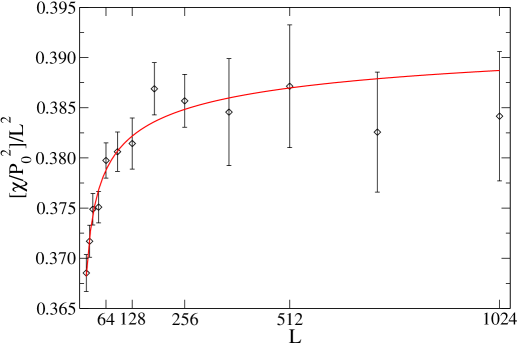
Figure 6: FSS of the combination $\chi(\beta,L)/P_{0}^{2}(\beta,L)$ at the asymptotic critical point $\beta_{c}=0.6931\ldots$ scaled by the leading $L^{2}$ behaviour to exhibit the corrections to scaling. The solid line shows a fit of the form (35) to the data.

3.2.4 FSS of the spontaneous polarization.

To derive FSS for the spontaneous polarization, consider the second form given in equation (8), $P_{0}^{1/2}=(2\pi/\lambda)^{1/2}[y^{1/4}+y^{9/4}+\ldots]$, which is rapidly convergent in the scaling window. The sub-leading terms in $y$ are strongly suppressed in the scaling regime and can be neglected compared to correction terms to follow. Using again the expansion of $y$ in terms of $\xi=\xi(\beta,\infty)$ and equation (26) for $\lambda(\xi)$, one arrives at

$$P_{0}(\beta,\infty)=A_{P_{0}}(4\xi)^{-\beta/\nu}(\ln 4\xi)^{\omega_{P_{0}}}\left[1-\frac{2}{3}(4\xi)^{-2}+\frac{4}{3}\frac{(4\xi)^{-2}}{\ln 4\xi}+\ldots\right],$$ (36)

with $A_{P_{0}}=4/\pi$, $\beta/\nu=1/2$ and $\omega_{P_{0}}=1$. Note that this (exact) form does not contain any corrections of the log-log type present in the XY model correlation function amitkadanoff . To test the sufficiency of this approximation, we again use an analytically generated, “artificial” series of scaling data, evaluating $P_{0}(\beta,\infty)$ exactly from (8) for the series of pseudo-critical temperatures defined by (25) for $\kappa=1$ and the exact expression (7) for $\xi=\xi(\beta,\infty)$. Fitting the form (36) without the corrections in square brackets to these data, taking $A_{P_{0}}$ and $\beta/\nu$ as fit parameters (holding $\omega_{P_{0}}=1$ fixed), we arrive at $\beta/\nu=0.5001$, which is clearly sufficiently close to the exact result in terms of the statistical accuracy to be expected from the simulation data. We thus conclude that the scaling corrections in square brackets of (36) can be neglected for our purposes.

Further FSS corrections arise from the behaviour (30) of the finite-size correlation length. For integer $\omega_{\xi}<0$ as indicated by the investigation of $\chi/P_{0}^{2}$ above, these corrections can be expanded in a power series,

$$P_{0}(\beta^{\ast},L)=A_{P_{0}}L^{-\beta/\nu}(\ln L)^{\omega_{P_{0}}}\left[1+\frac{B_{P_{0}}}{\ln L}+\frac{C_{P_{0}}}{(\ln L)^{2}}+\frac{D_{P_{0}}}{(\ln L)^{3}}\right],\;\;\;\omega_{\xi}<0,$$ (37)

where, again, the effect of the multiplier $\kappa$ is being incorporated in the correction amplitudes. For the case of a positive $\omega_{\xi}$, on the other hand, one would find a log-log correction to occur, i.e., one arrives at

$$P_{0}(\beta^{\ast},L)=A_{P_{0}}L^{-\beta/\nu}(\ln L)^{\omega_{P_{0}}-\omega_{\xi}/2}\left[1+B_{P_{0}}\frac{\ln\ln L}{\ln L}\right],\;\;\;\omega_{\xi}>0$$ (38)

where additionally, the exponent of the multiplicative logarithmic correction is “dressed” as $\omega_{P_{0}}-\omega_{\xi}/2$.

As for the route in the $(\beta^{\ast}(L),L)$ plane taken towards criticality, the two principal choices are given by the determination of $P_{0}(\beta^{\ast}=\beta_{c},L)$ at the fixed asymptotic critical coupling $\beta_{c}=\ln 2$ or by considering $P_{0}[\beta^{\ast}=\beta_{\chi}(L),L]$ at the polarizability peak locations $\beta_{\chi}(L)$. Asymptotically, both approaches should give compatible results; the strength and composition of scaling corrections, however, might be noticeably different. Following the first approach, we analyze the data from lattices of sizes $L=16,\ldots,1024$. Uncorrected fits of (37) with $B_{P_{0}}=C_{P_{0}}=D_{P_{0}}=0$ and omitted multiplicative correction term, i.e., $\omega_{P_{0}}=0$, yield exponents $\beta/\nu$ approaching the expected value logarithmically slow on successively omitting data points from the small-$L$ side of the list. For $L=92,\ldots,1024$, for instance, we find $\beta/\nu=0.4658(20)$, statistically incompatible with $\beta/\nu=1/2$. With variable $\omega_{P_{0}}$, on the other hand, the leading scaling exponent can be reasonably reproduced ($L_{\mathrm{min}}=24$),

$$\begin{array}[]{rcl}A_{P_{0}}&=&2.159(35),\\ \beta/\nu&=&0.4872(76),\\ \omega_{P_{0}}&=&0.109(33),\\ Q&=&0.14,\end{array}$$ (39)

but the resulting exponent of the logarithmic correction is estimated in strong deviation from $\omega_{P_{0}}=1$. This shortcoming can only be remedied by including the power-series type corrections in (37). Letting only $B_{P_{0}}$ vary, we arrive at estimates $\beta/\nu=0.50(60)$, $\omega_{P_{0}}=1.12(14)$, $Q=0.13$, which fit the expectations very well. In view of the large error estimates, however, one should not be deceived by the very small deviation from the exact result. In fact, even with $C_{P_{0}}=D_{P_{0}}=0$ still fixed, the $\chi^{2}$ distribution exhibits multiple local minima and the fit results heavily depend on the initial parameter values. Additionally letting $C_{P_{0}}$ and/or $D_{P_{0}}$ vary, the fits get very unstable and meaningful results can no longer be found. Using constraint fits, however, it can be clearly seen that the small value $\omega_{P_{0}}=0.109(33)$ above is indeed an effect of neglected higher-order scaling corrections: fixing $\beta/\nu=1/2$ as well as $\omega_{P_{0}}=1$ we determine the amplitudes $A_{P_{0}}$, $B_{P_{0}}$, $C_{P_{0}}$ and $D_{P_{0}}$ with $Q=0.26$. Now, fitting the form $E(\ln L)^{-\alpha}$ to the values of the thus determined polynomial $1+B_{P_{0}}(\ln L)^{-1}+C_{P_{0}}(\ln L)^{-2}+D_{P_{0}}(\ln L)^{-3}$, we find $\alpha\approx 0.83$. Thus, neglecting the scaling corrections in square brackets of (37) clearly leads to an effective reduction of the exponent estimate $\omega_{P_{0}}$ from its asymptotic value $\omega_{P_{0}}=1$ by about $\alpha\approx 0.8-0.9$.

Considering the spontaneous polarization at the peak positions of the polarizability for lattice sizes up to $L=256$, the uncorrected form with $\omega_{P_{0}}=B_{P_{0}}=C_{P_{0}}=D_{P_{0}}=0$ yields very small estimates for $\beta/\nu$ around $\beta/\nu\approx 0.25$ slowly increasing with the cutoff $L_{\mathrm{min}}$. Including the multiplicative logarithmic correction of equation (37), i.e., relaxing the constraint $\omega_{P_{0}}=0$, these results can be improved, and, e.g., for $L_{\mathrm{min}}=92$, we find the following fit parameters,

$$\begin{array}[]{rcl}A_{P_{0}}&=&1.49(50),\\ \beta/\nu&=&0.44(11),\\ \omega_{P_{0}}&=&0.71(55),\\ Q&=&0.57,\end{array}$$ (40)

with an exponent estimate for $\beta/\nu$ well compatible with the exact result $\beta/\nu=1/2$, although endowed with an unpleasantly large statistical error. The inclusion of the power-series type scaling corrections of (37) necessary for a full resolution of the corrections is not possible with the present data. Fixing $\beta/\nu=1/2$, $\omega_{P_{0}}=1$, however, these terms provide an excellent description for the present scaling corrections and a quality-of-fit $Q=0.72$ is already attained for $L_{\mathrm{min}}=16$ (including all three terms $B_{P_{0}}$, $C_{P_{0}}$ and $D_{P_{0}}$). In general, fits to the data at the maxima of the polarizability are found to be somewhat less stable and precise than those to the data at $\beta_{c}$, which we attribute to the smaller available system sizes here as well as additional scatter of the data due to the necessary reweighting.

In addition to the self-contained scaling routes in the $(\beta^{\ast}(L),L)$ plane described, for the exactly solved case considered here it is also possible to perform simulations for the analytical series $\beta^{\ast}(L)$ of inverse temperatures defined by the relation (25) with the exact expression (7) for $\xi$, which yields a scenario somewhat in between the $\beta^{\ast}(L)=\beta_{c}$ and $\beta^{\ast}(L)=\beta_{\chi}(L)$ cases. This artificial series of simulation data is indeed found to result in quite stable fits, such that at least the amplitude $B_{P_{0}}$ of (37) can be left variable to yield $\beta/\nu=0.51(47)$, $\omega_{P_{0}}=1.1(69)$ with $Q=0.66$ and $L_{\mathrm{min}}=16$. It should be noted that also fits of the form (38) with a log-log correction are possible with good quality for the scaling of the polarization, which only very slightly change the estimates for $\beta/\nu$, but do not lift the estimate for $\omega_{P_{0}}$ to the expected value $\omega_{P_{0}}=1$. Thus, it would be hard to distinguish the forms (37) and (38) solely on the basis of the numerical polarization data.

3.2.5 FSS of the polarizability.

Since the staggered polarizability $\chi$ is not known exactly, a systematic discussion of $\chi$ as a function of the asymptotic correlation length $\xi$ is not possible. However, from Baxter’s conjecture (18) the leading behaviour is expected to be

$$\chi(\beta,\infty)=A_{\chi}\xi^{\gamma/\nu}(\ln\xi)^{\omega_{\chi}},$$ (41)

with $\gamma/\nu=1$ and $\omega_{\chi}=2$. Repeating the arguments presented above for the polarization, again assuming an integer $\omega_{\xi}<0$ in equation (30), one deduces the following FSS ansatz,

$$\chi(\beta^{\ast},L)=A_{\chi}L^{\gamma/\nu}(\ln L)^{\omega_{\chi}}\left[1+\frac{B_{\chi}}{\ln L}+\frac{C_{\chi}}{(\ln L)^{2}}+\frac{D_{\chi}}{(\ln L)^{3}}\right],\;\;\;\omega_{\xi}<0,$$ (42)

whereas $\omega_{\xi}>0$ would result in a form including a log-log correction as in (38). We first investigate the simulation results at criticality, using data from lattices of sizes $L=16,\ldots,1024$. From fits of the leading scaling behaviour dropping the multiplicative and additive logarithmic correction terms, $\omega_{\chi}=0$ and $B_{\chi}=C_{\chi}=D_{\chi}=0$, to these data, we find reasonable fit qualities only when dropping many points from the small-$L$ side of the size range. Successively increasing the cutoff $L_{\mathrm{min}}$ a very slow downward drift of the estimates for $\gamma/\nu$ is observed. For $L_{\mathrm{min}}=92$, we arrive at an estimate $\gamma/\nu=1.0754(22)$ with $Q=0.96$, which is clearly incompatible with the exact result in terms of the statistical error. Letting $\omega_{\chi}$ vary while still keeping $B_{\chi}=C_{\chi}=D_{\chi}=0$ fixed, stable and good-quality fits can be attained. For the range $L=24,\ldots,1024$, we have

$$\begin{array}[]{rcl}A_{\chi}&=&1.581(31),\\ \gamma/\nu&=&1.0166(90),\\ \omega_{\chi}&=&0.320(40),\\ Q&=&0.78,\end{array}$$ (43)

in good agreement with the exact result $\gamma/\nu=1$, however, again clearly missing the expected asymptotic value of the exponent of the multiplicative logarithmic correction, $\omega_{\chi}=2$. The scaling plot presented in figure 7 shows this last fit together with the simulation data, scaled such as to expose the magnitude of scaling corrections present. The asymptotic value $\omega_{\chi}=2$ could be recovered by including the correction amplitudes $B_{\chi}$, $C_{\chi}$ and $D_{\chi}$. Letting only $B_{\chi}$ additionally vary, $\omega_{\chi}$ is already increased to $\omega_{\chi}=1.32(17)$ with $\gamma/\nu=1.0(48)$, $Q=0.78$ and $L_{\mathrm{min}}=16$. The obviously necessary higher-order terms $C_{\chi}$ and $D_{\chi}$ unfortunately cannot be fitted any more with the present data, however. On the other hand, fixing again $\gamma/\nu=1$ and $\omega_{\chi}=2$, the present corrections can be well described by the amplitudes $B_{\chi}$, $C_{\chi}$, $D_{\chi}$, resulting in a quality-of-fit of $Q=0.84$ already for $L_{\mathrm{min}}=16$. We note that here even the inclusion of the $(\ln L)^{-3}$ term $D_{\chi}$ is probably crucial since the leading multiplicative logarithmic correction is already quadratic.

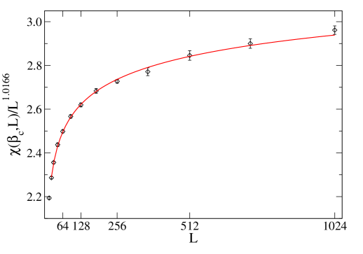
Figure 7: Finite-size scaling plot of the critical staggered polarizability $\chi(\beta_{c},L)$ for lattice sizes from $L=16$ up to $L=1024$. The solid line shows a fit of the functional form (42) with $B_{\chi}=C_{\chi}=D_{\chi}=0$ to the data. The abscissa has been re-scaled such as to factor out the leading scaling behaviour $\propto L^{\gamma/\nu}$ with $\gamma/\nu=1.0166$ from the fit (43).

Estimates of the maxima $\chi[\beta_{\chi}(L),L]$ are available for lattice sizes $L=16,\ldots,256$. A reasonable quality fit of the uncorrected form (42) with $\omega_{\chi}=0$ and $B_{\chi}=C_{\chi}=D_{\chi}=0$ to these data can be produced starting from $L_{\mathrm{min}}=64$, which yields an estimate $\gamma/\nu=1.2788(58)$, $Q=0.23$, lying even much further off the asymptotic result than in the case of the critical polarizability. Letting $\omega_{\chi}$ vary while keeping $B_{\chi}=C_{\chi}=D_{\chi}=0$ fixed, the estimate for $\gamma/\nu$ is noticeably reduced to $\gamma/\nu=1.13(08)$ with $\omega_{\chi}=0.71(36)$, $Q=0.15$, for $L_{\mathrm{min}}=46$, and a further tendency to decrease on an increase of $L_{\mathrm{min}}$ remains. Although here again, the need for higher-order correction terms is apparent, we find the data not precise enough for their inclusion. Thus, although both methods, consideration of the critical polarizability as well as scaling of the peak heights of $\chi(L)$, yield equivalent results, we find corrections to scaling slightly more pronounced in the latter approach. This is partly explained by the fact that for $\chi(\beta_{c},L)$ larger lattice sizes could be considered. However, even restricting a fit with $B_{\chi}=C_{\chi}=D_{\chi}=0$ for $\chi(\beta_{c},L)$ to $L\leq 256$, we find with $\gamma/\nu=1.006(11)$ for $L_{\mathrm{min}}=16$ a considerably more precise result closer to the asymptotic value; additionally, as mentioned above, no further drift of $\gamma/\nu$ is noticeable there as $L_{\mathrm{min}}$ is increased. For the extra simulation series at inverse temperatures $\beta^{\ast}(L)$ resulting from equation (25) with $\kappa=1$, a fit with $B_{\chi}=C_{\chi}=D_{\chi}=0$ and $L_{\mathrm{min}}=32$ leads to $\gamma/\nu=1.075(66)$, $\omega_{\chi}=1.21(29)$ with $Q=0.48$. Inclusion of the $B_{\chi}$, $C_{\chi}$ and $D_{\chi}$ terms destabilizes the fits too far, although consistency with $\gamma/\nu=1$, $\omega_{\chi}=2$ is again found on fitting the amplitudes only.

3.2.6 The scaling dimension in the critical phase.

Due to the criticality of the high-temperature phase one expects scaling and, accordingly, FSS in the whole region $\beta<\beta_{c}=\ln 2$. The closed-form conjecture (19) for the exponent $\eta$ entails predictions for the FSS of $P_{0}(\beta,L)$ and $\chi(\beta,L)$ for $\beta<\beta_{c}$. In terms of the scaling dimension $x_{P}=\beta/\nu=1-\gamma/2\nu$ henkel:book and the inverse temperature $\beta$, equation (19) reads

$$x_{P}(\beta<\beta_{c})=\frac{\pi}{2}\left\{\mathrm{arccos}[1-\frac{1}{2}\exp(2\beta)]\right\}^{-1},$$ (44)

which behaves close to the critical point $\beta_{c}=\ln 2$ as

$$x_{P}(\beta)=\frac{1}{2}+\frac{\sqrt{2}}{\pi}(\ln 2-\beta)^{1/2}+{\cal O}(\ln 2-\beta),$$ (45)

such that $x_{P}$ has a vertical tangent at $\beta_{c}$, implying an especially sensitive dependence of $x_{P}$ on scaling corrections there. It is worthwhile to notice that, although the correspondence between the XY and $F$ models only applies to their critical points, an analogous square-root singularity of the exponent $\eta$ of the XY model is found on entering the critical low-temperature phase there, see, e.g., reference res:00a . The leading scaling behaviour of $P_{0}(\beta,L)$ and $\chi(\beta,L)$ for $\beta<\beta_{c}$ is hence expected to be

$$\begin{array}[]{rcl}P_{0}(\beta,L)&=&A_{P_{0}}L^{-x_{P}(\beta)},\\ \chi(\beta,L)&=&A_{\chi}L^{2-2x_{P}(\beta)}.\end{array}$$ (46)

The solid lines of figure 8 illustrate the predicted behaviour of these exponents in the high-temperature phase. As can be seen, the polarizability exponent $2-2x_{P}(\beta)$ crosses zero at the free-fermion coupling $\beta_{f}=\frac{1}{2}\ln 2$ and, consequently, $\chi$ should be non-divergent below. As a result, the predicted singularity would be covered by non-singular background terms there, such that we restrict ourselves to the range $\beta_{f}\leq\beta\leq\beta_{c}$ here.

\psfrag{this is fit number one or somethin}{\small$x_{P}$ from fits to (\ref{eq:corrected_critical_phase_scaling})}\psfrag{this is fit number two}{\small$x_{P}$ from fits to (\ref{eq:leading_critical_phase_scaling})}\psfrag{this is fit number three}{\small$2-2x_{P}$ from fits to (\ref{eq:leading_critical_phase_scaling})}\psfrag{this is fit number four}{\small$2-2x_{P}$ from fits to (\ref{eq:corrected_critical_phase_scaling})}\includegraphics[clip={true},keepaspectratio={true},width=270.30118pt]{critical_phase_gamma}

Figure 8: Finite-size scaling dimensions $x_{P}(\beta)$ of the spontaneous staggered polarization and $2-2x_{P}(\beta)$ of the staggered polarizability, respectively, as a function of inverse temperature $\beta$ in the critical phase $\beta<\beta_{c}$. The symbols denote results from FSS fits of the functional forms (46) resp. (47) with $B=C=D=0$ to the simulation data. The solid lines correspond to the conjecture (44) for the analytic form. The vertical dashed lines indicate the locations of the the free-fermion point $\beta_{f}=\frac{1}{2}\ln 2$ and the critical point $\beta_{c}=\ln 2$, respectively.

Table 3: Fit parameters for $P_{0}$ and $\chi$ in the critical phase $\beta_{f}\leq\beta\leq\beta_{c}$. (a) Fits of the form (46). (b) Fits of the form (47) with $B=C=D=0$. (c) Fits of the form (47) with $D=0$ and $x_{P}$ fixed at the values (44). (d) Fits of the form (47) with $D=0$ and $\omega_{P_{0}}=1$ resp. $\omega_{\chi}=2$ fixed.

	conj.		(a)			(b)					(c)				(d)
$\beta$	$x_{P}$		$x_{P}$		$L_{\mathrm{min}}$	$x_{P}$		$\omega_{P_{0}}$		$L_{\mathrm{min}}$	$\omega_{P_{0}}$		$Q$		$x_{P}$		$Q$
$\ln 2$	0.	500	0.	4643(27)	128	0.	487(08)	0.	109(33)	24	1.	16(32)	0.	11	0.	48(62)	0.	20
0.65	0.	614	0.	5940(18)	128	0.	626(22)	0.	18(12)	92	1.	01(18)	0.	47	0.	61(44)	0.	44
0.60	0.	685	0.	6753(15)	182	0.	710(17)	0.	212(96)	92	0.	95(15)	0.	61	0.	69(38)	0.	67
0.55	0.	749	0.	7334(12)	128	0.	761(17)	0.	161(94)	92	1.	00(17)	0.	45	0.	75(40)	0.	45
0.50	0.	811	0.	7917(15)	182	0.	851(12)	0.	354(66)	92	1.	04(15)	0.	59	0.	81(36)	0.	49
0.45	0.	871	0.	8411(14)	182	0.	874(15)	0.	206(85)	92	1.	11(15)	0.	02	0.	86(34)	0.	01
0.40	0.	933	0.	8835(14)	182	0.	954(11)	0.	424(60)	64	1.	26(19)	0.	55	0.	91(25)	0.	10
0.35	0.	996	0.	9238(18)	256	0.	997(11)	0.	456(61)	64	1.	46(22)	0.	74	0.	95(21)	0.	07
$\beta$	$2-2x_{P}$		$2-2x_{P}$		$L_{\mathrm{min}}$	$2-2x_{P}$		$\omega_{\chi}^{\prime}$		$L_{\mathrm{min}}$	$\omega_{\chi}$		$Q$		$2-2x_{P}$		$Q$
$\ln 2$	1.	000	1.	0746(28)	128	1.	017(09)	0.	32(04)	24	2.	50(12)	0.	91	0.	96(309)	0.	53
0.65	0.	772	0.	8206(35)	182	0.	726(34)	0.	56(19)	92	2.	81(11)	0.	24	0.	66(320)	0.	26
0.60	0.	629	0.	6593(32)	182	0.	607(46)	0.	32(26)	128	2.	85(08)	0.	99	0.	51(640)	0.	45
0.55	0.	502	0.	5386(21)	128	0.	466(31)	0.	42(18)	92	2.	80(08)	0.	79	0.	39(668)	0.	11
0.50	0.	379	0.	4211(31)	182	0.	304(34)	0.	70(19)	92	2.	64(14)	0.	75	0.	28(825)	0.	73
0.45	0.	257	0.	3165(33)	182	0.	239(36)	0.	50(21)	92	2.	93(10)	0.	03	0.	17(1132)	0.	01
0.40	0.	134	0.	2265(44)	256	0.	098(23)	0.	81(13)	64	2.	81(20)	0.	83	0.	08(1362)	0.	85
0.35	0.	009	0.	1508(40)	256	0.	011(16)	0.	88(09)	46	2.	85(26)	0.	56	0.	00(1478)	0.	64

To test the form (44) we performed seven series of simulations at inverse temperatures $\beta=0.35,0.40,\ldots,0.65$ with the same series of system sizes $L=16,\ldots,1024$ used at $\beta=\ln 2$. Fitting the expected leading scaling behaviour (46) to the simulation data, many system sizes from the small-$L$ side have to be dropped to reach satisfactory fit qualities and to account for the observed slow drift of the resulting scaling exponents on increasing $L_{\mathrm{min}}$, which was finally chosen to be $L_{\mathrm{min}}=182$ in most cases, cf. the data in column (a) of table 3. As can be seen from the fit data presented in figure 8, even with this precaution highly significant deviations of the fit results from equation (44) are observed, especially close to the free-fermion coupling $\beta_{f}$. Scaling corrections are assumed here to take the form found at criticality, i.e.,

$$\begin{array}[]{rcl}P_{0}(\beta,L)&=&\displaystyle A_{P_{0}}L^{-x_{P}(\beta)}(\ln L)^{\omega_{P_{0}}(\beta)}\left[1+\frac{B_{P_{0}}}{\ln L}+\frac{C_{P_{0}}}{(\ln L)^{2}}+\frac{D_{P_{0}}}{(\ln L)^{3}}\right],\\[7.5347pt] \chi(\beta,L)&=&\displaystyle A_{\chi}L^{2-2x_{P}(\beta)}(\ln L)^{\omega_{\chi}(\beta)}\left[1+\frac{B_{\chi}}{\ln L}+\frac{C_{\chi}}{(\ln L)^{2}}+\frac{D_{\chi}}{(\ln L)^{3}}\right].\end{array}$$ (47)

As for the critical polarization and polarizability, fits including all of the correction terms (amounting to six variable parameters) are not possible with the available data. Including only the multiplicative logarithmic correction with variable exponent $\omega_{P_{0}}$ resp. $\omega_{\chi}$, we arrive at largely improved estimates for the scaling dimension $x_{P}$ in agreement with the prediction (44), see the column (b) of table 3 and the data in figure 8. The values of the correction exponents $\omega_{P_{0}}$ resp. $\omega_{\chi}$, however, again have to be considered as effective exponents owed to the omission of the additive corrections $B$, $C$, $D$. Note that in principle also the values of $\omega_{P_{0}}$ resp. $\omega_{\chi}$ could depend on the value of the coupling $\beta$ as indicated in equation (47). To investigate this possibility, we performed fits with the leading scaling exponents fixed to the presumably exact values of $x_{P}$ from (44), letting $\omega_{P_{0}}$ resp. $\omega_{\chi}$ vary and including two orders of additive scaling corrections, i.e., enforcing $D=0$ only. The results of these fits are collected in column (c) of table 3. In all cases with the exception of $\beta=0.45$, which seems to be an outlier, we find very good fit qualities, again indicating consistency with the conjecture (44). The estimates for $\omega_{P_{0}}$ are all consistent with a constant value of $\omega_{P_{0}}=1$, independent of the coupling $\beta$. The estimates for $\omega_{\chi}$, on the other hand, are clearly larger than $\omega_{\chi}=2$, but no general trend on varying $\beta$ is observed. This deviation of $\omega_{\chi}$ is found to disappear upon inclusion of the next-order correction amplitude $D_{\chi}$ for which, however, both exponents, $x_{P}$ and $\omega_{\chi}$, have to be kept fixed. This term has to be included here but not for the polarization since for $\chi$ already the leading multiplicative logarithmic correction is quadratic. When fixing both exponents, $x_{P}$ and $\omega$, fits of good quality are attained for both observables and all couplings $\beta$ on including all three additive correction terms of (47). In passing we note that an analysis of $\chi/P_{0}^{2}$ in the critical phase yields negative values of $\omega_{\xi}$ everywhere and fits of the power-law form (35) describe the corrections extremely well.

3.3 Results of the Thermal Scaling Analysis

The discussed FSS of the critical polarization and polarizability is independent of the value of the critical exponent $\rho$. For the scaling of the polarizability peak positions in section 3.2.2, on the other hand, the need to resolve the present strong logarithmic scaling corrections did not allow for an additional independent determination of $\rho$. To directly verify the exponential type of the observed divergences and to estimate the parameter $\rho$, one should hence consider thermal instead of finite-size scaling. Figure 9 shows an overview of the temperature dependence of the staggered polarizability for different lattice sizes. The clear scaling of $\chi$ for the high-temperature region $\beta<\beta_{c}=\ln 2$ illustrates again the presence of a critical phase. In contrast, for the low-temperature phase to the right of the peaks, the polarizability curves essentially collapse and only start to disagree as the correlation length reaches the linear extent of the considered lattice. Therefore, a thermal scaling analysis must be performed in the low-temperature vicinity of the critical point, the behaviour in the high-temperature phase being completely governed by finite-size effects. Here, we do not consider the scaling of the correlation length itself, but instead analyze the thermal scaling of the spontaneous polarization and the polarizability for a single lattice of size $L=256$. Simulations were performed for a closely spaced series of temperatures in the low-temperature vicinity of the critical point.

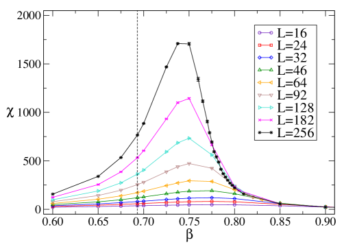
Figure 9: Scaling of the polarizability peaks from simulation data. The lines simply connect the data points and are drawn to guide the eye. The dashed vertical line indicates the location of the asymptotic critical coupling $\beta_{c}=0.6931\ldots$

3.3.1 Scaling of the spontaneous polarization.

From the leading term of (8) in $y$ and the dependence of $\lambda$ on $\beta$, the spontaneous polarization behaves as

$$P_{0}(\beta) = \frac{\pi}{\sqrt{2}}\left[(\beta-\beta_{c})^{-1/2}-\frac{1}{6}(\beta-\beta_{c})^{1/2}+\ldots\right]$$ (48)

$$\times\exp\left\{-\frac{\pi^{2}}{8\sqrt{2}}\left[(\beta-\beta_{c})^{-1/2}-\frac{1}{6}(\beta-\beta_{c})^{1/2}+\ldots\right]\right\}$$

as $\beta_{c}$ is approached from above. Taking only the leading-order terms into account, we consider the following scaling form,

$$\ln P_{0}(\beta)=A_{P_{0}}+B_{P_{0}}(\beta-\beta_{c})^{-\rho}+C_{P_{0}}\ln(\beta-\beta_{c}),$$ (49)

with $C_{P_{0}}=-1/2$ and $\rho=1/2$. The window of validity of (49) for the thermal scaling of $P_{0}$ for a finite lattice is limited for small deviations $\beta-\beta_{c}$ by finite-size effects and for large deviations $\beta-\beta_{c}$ by the higher-order corrections to scaling indicated in (48). If correlation lengths are measured, one might monitor the effect of the finite lattice size by comparing the value of the correlation length $\xi(\beta,L)$ at a given $\beta>\beta_{c}$ with the linear extent $L$ of the lattice wj:93a . Here, the onset of finite-size effects is estimated by the beginning of the rounding of the exponential decline of $P_{0}$ as $\beta_{c}$ is approached. From monitoring the quality-of-fit parameter and estimation of the onset of the finite-size rounding, we determine a fit range of $\beta_{\mathrm{min}}=0.77\leq\beta\leq 0.85=\beta_{\mathrm{max}}$. We find fits of the full five-parameter family (49) of functions to the data possible, but the resulting fit parameters are endowed with astronomic error estimates and the corresponding $\chi^{2}$ distribution has multiple minima such that different “solutions” can be found. We thus fix one or two of the parameters at their expected asymptotic values to reach more stable fits, cf. the fit data collected in table 4. Note that the parameters of the fully unrestricted fit where found starting from the parameters of one of the restricted fits, thus explicitly selecting one of the $\chi^{2}$ minima. Figure 10 shows the simulation data together with this unrestricted fit and the exact asymptotic polarization of (8). The vertical line denotes the inverse temperature $\beta^{\ast}$ where the asymptotic correlation length $\xi(\beta^{\ast},\infty)$ of equation (7) reaches the linear size $L=256$ of the system. As expected, this point approximately coincides with the inverse temperature where the simulation data deviate from the asymptotic result due to finite-size effects, thus justifying the method of determining $\beta_{\mathrm{min}}$. The inset of figure 10 shows the approximation of (48) with only the first-order terms of both expansions being kept in comparison to the full asymptotic result (8) and the simulation data. As can be seen, even in the scaling range considered here, the deviation is much larger than the statistical errors of the data. The observed shift, however, can be mostly reproduced by slight changes of the amplitudes $A_{P_{0}}$ and $B_{P_{0}}$, such that (49) still fits the data well. The fitted amplitudes $A_{P_{0}}$, $B_{P_{0}}$ and $C_{P_{0}}$ must be considered effective, however, and deviations of the fitted parameters from the exact asymptotic values are due to the effective inclusion of neglected higher-order correction terms.

Table 4: Parameters of fits of the form (49) for $P_{0}$ (upper part) resp. the form (50) for $\chi$ (lower part) to the simulation data. Values in square brackets indicate that the corresponding parameter was held fixed in the fit procedure.

$A_{P_{0}}$		$B_{P_{0}}$		$C_{P_{0}}$		$\beta_{c}$		$\rho$		$Q$
0.	8(147)	$-0$.	7(156)	$-0$.	2(57)	0.	706(85)	0.	5(32)	0.	79
1.	67(35)	$-1$.	59(31)	[$-0$.	5]	0.	7089(39)	0.	339(44)	0.	86
0.	736(15)	$-0$.	803(11)	[$-0$.	5]	[0.	69315]	0.	522(33)	0.	14
0.	8088(47)	$-0$.	8616(22)	[$-0$.	5]	0.	69499(27)	[0.	5]	0.	23
0.	691(30)	$-0$.	579(78)	$-0$.	199(85)	0.	7055(32)	[0.	5]	0.	85
$A_{\chi}$		$B_{\chi}$		$C_{\chi}$		$\beta_{c}$		$\rho$		$Q$
0.	5(13)	0.	15(31)	[$-1$.	0]	0.	62(13)	1.	8(18)	0.	13
$-1$.	03(21)	0.	88(12)	[$-1$.	0]	[0.	69315]	0.	699(37)	0.	11
$-1$.	95(11)	1.	549(57)	[$-1$.	0]	0.	7046(19)	[0.	5]	0.	08
$-2$.	2(154)	2.	4(179)	0.	005(9299)	[0.	69315]	0.	5(12)	0.	08
0.	5(24)	0.	6(12)	[0.	0]	0.	647(92)	1.	2(13)	0.	13
$-2$.	18(38)	2.	37(27)	[0.	0]	[0.	69315]	0.	520(27)	0.	12
$-2$.	38(13)	2.	531(66)	[0.	0]	0.	6944(19)	[0.	5]	0.	12

3.3.2 Scaling of the polarizability

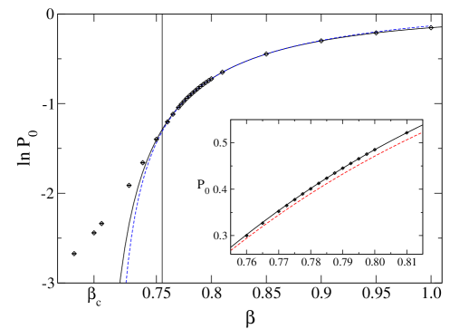
Figure 10: Thermal behaviour of the spontaneous staggered polarization $P_{0}$ close to $\beta_{c}$ from simulations of a $256^{2}$ system. The solid line denotes the exact asymptotic result (8), the dashed line is a fit of the form (49) to the data. The vertical line denotes the point where $\xi(\beta^{\ast},\infty)=L=256$. The inset shows the exact solution (8) compared to the first-order approximation of (48) in the inverse temperature regime used for the fit.

From the conjecture (18) for the near-critical polarizability, we expect $\chi(\beta)$ to scale analogous to the polarization,

$$\ln\chi(\beta)=A_{\chi}+B_{\chi}(\beta-\beta_{c})^{-\rho}+C_{\chi}\ln(\beta-\beta_{c}),$$ (50)

where the differences to the scaling of $P_{0}$ only show up in the amplitudes $A_{\chi}$, $B_{\chi}$ and $C_{\chi}=-1$. From the flattening out of the exponential divergence near $\beta_{c}$ and by monitoring the quality of fit, we estimate the same scaling window $\beta_{\mathrm{min}}=0.77\leq\beta\leq 0.85=\beta_{\mathrm{max}}$ for (50) we encountered for the polarization. We find fits for the polarizability to be considerably less stable than those for the polarization, and we did not succeed to fit all five parameters independently. Fixing $C_{\chi}=-1$, a reasonable result for $\rho$ cannot be found, even when additionally fixing $\beta_{c}=\ln 2$, cf. the data compiled in table 4. Since a fit with only $\beta_{c}$ fixed yields $C_{\chi}\approx 0$, corresponding to an omission of this correction term, we also tried fits with $C_{\chi}=0$ fixed, which work considerably better than fits with $C_{\chi}=-1$. However, still meaningful results for $\rho$ and $\beta_{c}$ can only be found when fixing one of the two parameters, which then yields good agreement with the asymptotic result. Figure 11 shows the simulation data together with a fit with $C_{\chi}=0$ and $\beta_{c}=\ln 2$ fixed. Comparison of the asymptotic correlation length (7) with the system size $L=256$ indicates the approximate onset of finite-size effects as the critical point is approached.

To see in how far it is possible to distinguish the occurring essential singularity from a conventional power-law behaviour, we also performed fits to the form (50) with the left side replaced by $\chi(\beta)$ instead of $\ln\chi(\beta)$ and $C_{\chi}=0$ held fixed. With this power-law form and the same range of inverse temperatures used for the exponential fits, we arrive at the following parameters,

$$\begin{array}[]{rcl}A^{\prime}_{\chi}&=&13.5(49),\\ B^{\prime}_{\chi}&=&0.040(35),\\ \beta_{c}&=&0.7112(96),\\ \rho^{\prime}&=&3.54(51),\\ Q&=&0.13,\end{array}$$ (51)

where $\rho^{\prime}$ now would correspond to the conventional critical exponent $\gamma$ for the case of a finite-order phase transition. Thus, in agreement with the experience from the two-dimensional XY model, power-law fits can be performed with satisfactory quality if one accepts “unnaturally” large exponents such as $\rho^{\prime}=3.5$ here.

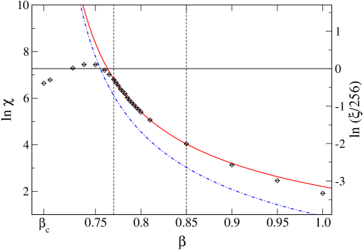
Figure 11: Thermal scaling of the polarizability on a $L=256$ lattice. The solid curve shows a fit of the functional form (50) to the data, where the parameters $C_{\chi}=0$ and $\beta_{c}=\ln 2$ were kept fixed. The vertical dashed lines indicate the window of data points included in the fit. To judge the onset of finite-size effects, the dashed-dotted curve shows the logarithm of the ratio $\xi(\beta,\infty)/L$ from equation (7), such that strong size effects are expected to appear as soon as $\ln[\xi(\beta,\infty)/L]\gtrsim 0$ (right scale).

4 Conclusions

We have considered the behaviour of the six-vertex $F$ model on the square-lattice at its Berezinskii-Kosterlitz-Thouless (BKT) point and within the critical high-temperature phase with a series of cluster-update Monte Carlo simulations and subsequent finite-size and thermal scaling analyses. Due to the presence of strong logarithmic corrections indicated by the exact solution and expected for a theory with central charge $c=1$, the scaling analysis has to carefully take correction terms into account and/or treat the presence of (even higher-order) corrections by omission of simulation points close to the border of the scaling region. Although the usefulness of the finite-size scaling (FSS) technique has been called into question at a BKT point due to the occurrence of essential singularities and most studies of the XY model case solely consider thermal scaling instead wj:93a , we find a FSS analysis for the $F$ model well possible and useful, as long as corrections to scaling are thoroughly included. The full FSS forms including the correction terms are explicitly derived from the exact results augmented by the plausible assumption (30) about the scaling of the finite-size correlation length. The latter is being confirmed by the analysis of a combination of observables proportional to a power of the correlation length without multiplicative logarithmic corrections, providing evidence that the finite-size correlation length exhibits additive logarithmic corrections in the present case (as opposed to multiplicative logarithmic corrections such as, e.g., at the upper critical dimension kenna:04a ). Due to the ambitious nature of many of the fits involved, however, one has to cope with the occurrence of competing local minima of the $\chi^{2}$ distribution and a distinctive flatness of these minima in some parameter directions entailed by the slow variation of the logarithmic terms. We would like to stress that the quality-of-fit parameter $Q$ is found to be not always sufficient for the detection of neglected higher-order corrections. Omitting the discussed correction terms, however, the resulting estimates do not even satisfy moderate expectations of accuracy and are strongly biased. For the FSS analysis the knowledge of the exact asymptotic critical coupling $\beta_{c}$ turns out to be highly beneficial and the results found from the scaling at effective pseudo-critical points are much less accurate. This might be taken as a caveat for simulations of the XY model, where $\beta_{c}$ is not exactly known. The correction exponents $\omega_{P_{0}}$ for the polarization and $\omega_{\chi}$ for the polarizability could not be consistently and accurately determined in fully unrestricted fits, although constrained fits including further correction terms allow to establish consistency with the analytical solution. This experience is shared with simulational studies of the XY model wj:97b , hasenbusch:05a . A thermal scaling analysis of the low-temperature approach towards criticality does only lead to reasonably precise results for the present data if at least one of the fit parameters is fixed to its exact value. A conventional algebraic singularity also fits to the data, but only when unusually large exponents are accepted.

In addition to the analysis at criticality, we consider the scaling of the polarization and the polarizability within the critical high-temperature phase. We find overall good agreement of the outcome with a conjecture youngblood , bogoliubov:84a for the behaviour of the scaling dimension $x_{P}(\beta)$ of the polarization in the critical phase, although the resolution of scaling corrections appears to be even more involved here than at criticality. Close to the critical point scaling corrections are especially pronounced, since the scaling dimension $x_{P}(\beta)$ turns out to have a vertical tangent at $\beta_{c}$. This might also contribute to the relatively poor outcome of the FSS analysis of the peak heights of the polarizability. With respect to the values of the effective correction exponents $\omega$ found for $\beta<\beta_{c}$ (cf. table 3), we note comparing to the critical point behaviour that the nature of the corrections seems to be rather different in both cases, such that the effective correction exponents and amplitudes exhibit fast variation as the critical phase is entered, which is again related to the singularity of $x_{P}(\beta)$ at $\beta_{c}$.

Finally, from deliberately reducing our simulation data set, we note that including lattice sizes only up to, e.g., $L=128$, most of the estimates for $\beta_{c}$, $\gamma/\nu$, $\beta/\nu$, $x_{P}(\beta)$ and $\rho$ are not found to be compatible with the asymptotic results in terms of the statistical errors. Thus, consideration of large system sizes is crucial here for the resolution of scaling corrections, see also reference hasenbusch:05a . This explains troubles experienced in the numerical analysis of the $F$ model on a particular, annealed ensemble of fluctuating quadrangulations, which due to their intrinsic fractality only allow simulations of lattices with rather small effective linear extents weigel:04b . For a more detailed investigation of the thermal scaling properties an analysis involving measurements of the finite-size correlation length would be valuable. This, as well as the examination of the critical phase below the free-fermion point $\beta_{f}$, is left to a future investigation.

References

- [1] Pauling L 1935 J. Am. Chem. Soc. 57 2680
- [2] Rys F 1963 Helv. Phys. Acta 36 537
- [3] Baxter R J 1982 Exactly Solved Models in Statistical Mechanics (London: Academic Press)
- [4] Baxter R J 1970 Phys. Rev. B 1 2199
- [5] van Beijeren H 1977 Phys. Rev. Lett. 38 993
- [6] Levi A C and Kotrla M 1997 J. Phys.: Condens. Matter 9 299
- [7] Bogoliubov N M, Pronko A G and Zvonarev M B 2002 J. Phys. A 35 5525
-
[8]
Berezinskii V L 1971 Zh. Eksp. Teor. Fiz. 61 1144
Kosterlitz J M and Thouless D J 1973 J. Phys. C 6 1181
Kosterlitz J M 1974 J. Phys. C 7 1046 -
[9]
Gupta R, DeLapp J, Batrouni G G, Fox G C, Baillie C F and Apostolakis J 1988
Phys. Rev. Lett. 61 1996
Wolff U 1989 Nucl. Phys. B 322 759
Edwards R G, Goodman J and Sokal A D 1991 Nucl. Phys. B 354 289 - [10] Janke W and Nather K 1993 Phys. Rev. B 48 7419
- [11] Kenna R and Irving A C 1997 Nucl. Phys. B 485 583
- [12] Janke W 1997 Phys. Rev. B 55 3580
- [13] Henkel M 1999 Conformal Invariance and Critical Phenomena (Berlin/Heidelberg/New York: Springer)
-
[14]
Amit D J, Goldschmidt Y Y and Grinstein S 1980 J. Phys. A 13
585
Kadanoff L P and Zisook A B 1981 Nucl. Phys. B 180 61 - [15] Janke W and Kappler S 1997 J. Physique I 7 663
- [16] Balog J, Niedermaier M, Niedermayer F, Patrascioiu A, Seiler E and Weisz P 2001 Nucl. Phys. B 618 315
- [17] Hasenbusch M 2005 J. Phys. A 38 5869
- [18] Weigel M and Janke W 2005 Nucl. Phys. B 719 312
- [19] Evertz H G and Marcu M 1993 Computer Simulations in Condensed Matter Physics VI ed D P Landau, K K Mon and H B Schüttler (Berlin: Springer) p 109
- [20] Barkema G T and Newman M E J 1998 Phys. Rev. E 57 1155
- [21] Syljuasen O F and Zvonarev M B 2004 Phys. Rev. E 70 016118
- [22] Evertz H G and Marcu M 1993 Nucl. Phys. B (Proc. Suppl.) 30 277
- [23] Mazzeo G, Jug G, Levi A C and Tosatti E 1992 J. Phys. A 25 L967; 1994 Phys. Rev. B 49 7625
- [24] Hasenbusch M, Marcu M and Pinn K 1992 Nucl. Phys. B (Proc. Suppl.) 26 598; 1994 Physica A 208 124
- [25] Lieb E H 1967 Phys. Rev. 162 162; 1967 Phys. Rev. Lett. 18 1046; 1967 Phys. Rev. Lett. 19 108
- [26] Sutherland B 1967 Phys. Rev. Lett. 19 103
- [27] Baxter R J 1973 J. Phys. C 6 L94
-
[28]
Mermin N D and Wagner H 1966 Phys. Rev. Lett. 17 1133
Hohenberg P C 1967 Phys. Rev. 158 383 -
[29]
Bramwell S T and Holdsworth P C W 1994 Phys. Rev. B 49 8811
Bramwell S T, Fortin J Y, Holdsworth P C W, Peysson S, Pinton J F, Portelli B and Sellitto M 2001 Phys. Rev. E 63 041106 - [30] Loison D 1999 J. Phys.: Condens. Matter 11 L401
- [31] Barber M E 1983 in C Domb and J L Lebowitz (eds.), Phase Transitions and Critical Phenomena (New York: Academic Press) vol. 8 p. 146
- [32] Savit R 1980 Rev. Mod. Phys. 52 453
- [33] Suzuki M 1974 Prog. Theor. Phys. 51 1992
-
[34]
Youngblood R, Axe J D and McCoy B M 1980 Phys. Rev. B 21 5212
Youngblood R and Axe J D 1981 Phys. Rev. B 23 232 - [35] Bogoliubov N M, Izergin A G and Korepin V E 1984 Nucl. Phys. B 275 687
- [36] Henley C 2005 Phys. Rev. B 71 014424
- [37] Berche B 2004 J. Phys. A 36 585
- [38] Villain J 1975 J. Physique 36 581
- [39] Knops H J F 1977 Phys. Rev. Lett. 39 766
- [40] Nienhuis B 1987 in C Domb and J L Lebowitz (eds.), Phase Transitions and Critical Phenomena (London: Academic Press) vol. 11 p. 1
- [41] Domany E, Schick M, Walker J S and Griffiths R B 1981 Phys. Rev. B 18 2209
- [42] Baxter R J 1976 J. Phys. A 9 397
- [43] Evertz H G 2003 Adv. Phys. 52 1
- [44] Evertz H G, Lana G and Marcu M 1993 Phys. Rev. Lett. 70 875
- [45] Lieb E H and Wu F Y 1972 in C Domb and M S Green (eds.), Phase Transitions and Critical Phenomena (London: Academic Press) vol. 1 p. 331
- [46] Ferrenberg A M and Swendsen R H 1988 Phys. Rev. Lett. 61 2635
- [47] Kenna R 2004 Nucl. Phys. B 691 292
-
[48]
Balog J 2001 J. Phys. A 34 5237
Balog J, Knechtli F, Korzec T and Wolff U 2003 Nucl. Phys. B 675 555 - [49] Ballesteros H G, Fernández L A, Martín-Mayor V, Muñoz Sudupe A, Parisi G and Ruiz-Lorenzo J J 1998 Nucl. Phys. B 512 681
- [50] Bittner E, Janke W and Markum H 2002 Phys. Rev. D 66 024008
- [51] Salas J and Sokal A D 1997 J. Stat. Phys. 88 567
- [52] Res I and Straley J P 2000 Phys. Rev. B 61 14425