Analytical Investigation of Innovation Dynamics Considering Stochasticity in the Evaluation of Fitness

Abstract

We investigate a selection-mutation model for the dynamics of technological innovation, a special case of reaction-diffusion equations. Although mutations are assumed to increase the variety of technologies, not their average success (“fitness”), they are an essential prerequisite for innovation. Together with a selection of above-average technologies due to imitation behavior, they are the “driving force” for the continuous increase in fitness. We will give analytical solutions for the probability distribution of technologies for special cases and in the limit of large times.

The selection dynamics is modelled by a “proportional imitation” of better technologies. However, the assessment of a technology’s fitness may be imperfect and, therefore, vary stochastically. We will derive conditions, under which wrong assessment of fitness can accelerate the innovation dynamics, as it has been found in some surprising numerical investigations.

Introduction. Innovation dynamics has not only been studied by economists and social scientists (see Refs. in Hub ), but also recently attracted an increasing interest by physicists Hub ; Llas ; Guard . Ebeling et al., for example, investigate the competition of an innovation with already established technologies BrucEbJiMo96 ; Ebeling .

In a wider perspective, the selection-mutuation equations discussed in this manuscript are a special case of reaction-diffusion equations, where technological imitation processes are analogous to chemical reactions and diffusion originates from mutation processes. Due to their non-linearity, reaction-mutation equations are known to display interesting pattern-formation phenomena such as (spiral) waves react ; turing1 or Turing patterns turing1 ; turing2 . However, this subject will not be the focus of this paper. Instead, we will try to understand some surprising observations in a microsimulation model of innovation dynamics by Saam Saam .

Our innovation model assumes that the success of a company’s technology can be expressed by a “fitness” value $x$. The technologies of superior companies are imitated (copied) with a certain probability per unit time specified later. Moreover, all companies perform innovative activities, which are modeled by random mutations of the currently applied technologies. Assuming a Brownian motion for the mutation of fitness values, they change from some value $x$ at time $t$ to some other value $z$ at time $t+\Delta t$ with a Gaussian transition probability

$$p(z(t+\Delta t)|x(t))=\frac{\mbox{e}^{-[z(t+\Delta t)-x(t)]^{2}/(2\theta\nu\,\Delta t)}}{\sqrt{2\pi\theta\nu\,\Delta t}}\,.$$ (1)

Here, $\nu$ is the frequency, $\nu\,\Delta t$ the number and $\sqrt{\theta}$ the standard deviation (average size) of mutations. According to Eq. (1), mutations may be beneficial, but they may also decrease the fitness of technologies. Therefore, the observed increase in the average fitness would have to be a consequence of the assumed imitation of superior technologies.

Patents on the leading technologies could suppress such imitation and, therefore, potentially reduce the speed of innovation, i.e. the increase in the average fitness of technologies. However, under certain conditions, a misperception of fitness values Hub seems to neutralize or even over-compensate such a deceleration effect Saam . Our paper will try to achieve an analytical understanding of these interesting findings.

Formulation of the Innovation Model. For the sake of analytical treatment, let us assume a continuous spectrum of possible fitness values $x$. Moreover, let $P(x,t)\,dx$ represent the probability with which the applied technology of a company has a fitness value between $x$ and $x+dx$ at time $t$. In addition, we will assume that companies imitate technologies with a higher fitness $z>x$ and that the imitation rate increases proportionally with the related increase $z-x$ in success. If $z-x$ is negative, the imitation rate should be zero. Then, given the presently applied technology has the fitness $x$, the respective imitation rate $w_{1}(z|x,t)$ to copy another technology of fitness $z$, is game ; kluwer

$$w_{1}(z|x,t)=\lambda P(z,t)\max(z-x,0)\,,$$ (2)

as the imitation rate is proportional to the occurence probability density $P(z,t)$ of the imitated technology $z$. The parameter $\lambda>0$ has the meaning of an imitation frequency.

In order to calculate the change of the occurence probability density $P(x,t)$ due to imitation processes, we have to insert $w(z|x,t)=w_{1}(z|x,t)$ into the continuous master equation kluwer ; weidlich ; evolbook

$$\frac{dP(x,t)}{dt}=\int dz\,[w(x|z,t)P(z,t)-w(z|x,t)P(x,t)]\,,$$ (3)

which leads to

$$\frac{dP(x,t)}{dt} = \lambda\int dz\,P(x,t)P(z,t)$$ (4)

$$\quad\times\underbrace{[\max(x-z,0)-\max(z-x,0)]}_{=x-z}$$

$$= \lambda P(x,t)\bigg{[}x-\!\!\!\!\underbrace{\int dz\,zP(z,t)}_{\mbox{\footnotesize\rm=~{}av. fitness $\langle x\rangle_{t}$}}\!\!\!\bigg{]}\,,$$ (5)

because of the normalization condition $\int dz\,P(z,t)=1$. Equation (5) is related to the selection equation from evolutionary biology eigen ; evolbook and to the game-dynamical equations HoSi ; game ; kluwer . In order to take into account new inventions, with

$$w(z|x,t)=\lim_{\Delta t\rightarrow 0}\frac{p(z(t+\Delta t)|x(t))}{\Delta t}+w_{1}(z|x,t)$$ (6)

we will additionally assume random transitions to other technologies $z$ with the rate $w_{0}(z|x,t)=w(z|x,t)-w_{1}(z|x,t)$. According to this, we simply treat inventions as unbiased random mutations, which may either increase or decrease the fitness of the pursued technology, as in complex (technological) systems it is sometimes hard to judge before, whether some change will cause an improvement or not. Although the assumption of unbiasedness may be questioned, it is favorable to gain non-trivial conclusions. The resulting equation for the temporal change of $P(x,t)$ can be approximated by the following Fokker-Planck type of equation Risken :

$$\frac{\partial P(x,t)}{\partial t}=\lambda P(x,t)\bigg{[}x-\underbrace{\int dz\,zP(z,t)}_{=\langle x\rangle_{t}}\bigg{]}+D\frac{\partial^{2}P(x,t)}{\partial x^{2}}\,.$$ (7)

The quantity $D=\nu\theta/2$ has the meaning of a diffusion coefficient. For the mean fitness $\langle x\rangle_{t}$ one can derive the differential equation evolbook ; kluwer

$$\frac{d\langle x\rangle_{t}}{dt}=\lambda\mbox{Var}_{t}(x)\,,$$ (8)

while for the variance $\mbox{Var}_{t}(x)=\langle(x-\langle x\rangle_{t})^{2}\rangle_{t}$, we find

$$\frac{d\mbox{Var}_{t}(x)}{dt}=\lambda\langle(x-\langle x\rangle_{t})^{3}\rangle_{t}+2D\,.$$ (9)

The term $\langle(x-\langle x\rangle_{t})^{3}\rangle_{t}$ disappears if the distribution $P(x,t)$ has a vanishing skewness $\gamma$, e.g. for a Gaussian distribution. Equation (8) shows that the diversity Var${}_{t}(x)$ is a key factor for a high innovation speed $d\langle x\rangle_{t}/dt$.

Equation (7) can be viewed as a special case of reaction-diffusion equations react ; turing1 , where the diffusion term originates from mutations and the non-linear reaction term from imitative pair interactions game ; kluwer . It is known to have a complicated formal solution, which is uniquely determined by the initial condition evolbook ; kluwer . However, this does not help us, here. We are rather looking for a qualitative understanding of the dynamic solution and, where possible, for explicit analytical expressions. In the limiting case $\nu=0=D$ of no mutation and no diffusion, all companies will eventually imitate the technology with the highest fitness $x_{\rm max}$, i.e. $\lim_{t\rightarrow\infty}P(x,t)=\delta(x-x_{\rm max})$, where $\delta(x)$ denotes Dirac’s delta function. In the limiting case $\lambda=0$ of no imitation, Eq. (7) is just a linear diffusion equation, and its solution is a superposition of Gaussian distributions with a linearly-in-time increasing variance $2Dt$:

$$P(x,t)=\int dz\frac{P(z,0)}{\sqrt{4\pi Dt}}\,\mbox{e}^{-(x-z)^{2}/(4Dt)}\,.$$ (10)

If we initially have a two-point distribution $P(x,0)=p_{1}\delta(x-x_{1})+p_{2}\delta(x-x_{2})$ with $p_{1}+p_{2}=1$, both peaks will become broader due to diffusion similarly to Eq. (10). At the same time, however, imitation tends to favour the peak around the superior technology’s fitness, while the peak around the inferior technology’s fitness will eventually disappear. After some time, one finds a unimodal, almost Gaussian distribution, if $\lambda$ and $D$ are constant, see Fig. 1.

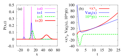
Figure 1: (Color Online)(a) Computer simulation of Eq. (7) with $D=1$ and $\lambda=0.1$. Starting with a two-peak initial distribution $P(x,0)$, one can see that the superposition law does not apply due to the non-linearity of our innovation model. Nevertheless, after some time ($t\geq 5$) we find the Gaussian distribution (11). (b) After the initially developing skewness $\gamma(t)=\langle(x-\langle x\rangle_{t})^{3}\rangle_{t}/\mbox{Var}_{t}(x)^{3/2}$ has vanished ($t\geq 5$), the variance Var${}_{t}(x)$ grows linearly and the mean fitness $\langle x\rangle_{t}$ quadratically, in accordance with Eqs. (16) and (17).

Therefore, let us investigate how a Gaussian distribution develops in time. We will show that the non-linear Eq. (7) has, then, a special solution of the form

$$P(x,t)=\frac{1}{\sqrt{2\pi g(t)}}\,\mbox{e}^{-[x-f(t)]^{2}/[2g(t)]}\,,$$ (11)

where $f(t)$ denotes the mean value and $g(t)$ the variance of the fitness values $x$. Applying the product, quotient, and chain rules of differential calculus, we find

$$\frac{\partial P(x,t)}{\partial x} = -\frac{2[x-f(t)]}{2g(t)}P(x,t)$$ (12)

$$\frac{\partial^{2}P(x,t)}{\partial x^{2}} = -\frac{1}{g(t)}P(x,t)+\left\{-\frac{2[x-f(t)]}{2g(t)}\right\}^{2}P(x,t)$$ (13)

$$= -\frac{1}{g(t)}P(x,t)+\frac{[x-f(t)]^{2}}{g(t)^{2}}P(x,t)$$

$$\frac{\partial P(x,t)}{\partial t} = -\frac{1}{2}\frac{\frac{dg}{dt}}{g(t)}P(x,t)+\frac{[x-f(t)]\frac{df}{dt}}{g(t)}P(x,t)$$ (14)

$$+ \frac{1}{2}\frac{\frac{dg}{dt}[x-f(t)]^{2}}{g(t)^{2}}P(x,t)\,.$$

Comparing the expression for $\partial P(x,t)/\partial t$ with the one for $\partial^{2}P(x,t)/\partial x^{2}$ shows that Eq. (11) implies

$$\frac{\partial P(x,t)}{\partial t}=\frac{\frac{dg(t)}{dt}}{2}\frac{\partial^{2}P(x,t)}{\partial x^{2}}+\frac{[x-f(t)]\frac{df(t)}{dt}}{g(t)}P(x,t)\,.$$ (15)

Considering $\langle(x-\langle x\rangle_{t})^{3}\rangle_{t}=0$, $f(t)=\langle x\rangle_{t}$, $g(t)=\mbox{Var}_{t}(x)$, and Eqs. (8), (9), this partial differential equation indeed agrees with Eq. (7). Therefore, Eq. (11) is the unique solution if the initial condition is a Gaussian distribution. The existence of such a generalized diffusion solution is quite surprising in view of the non-linearity of Eq. (7). This reminds one of the exact solution of the non-linear Burgers equation Burgers .

In the previously assumed case $D=\mbox{const.}$ of constant mutation activity, we obtain

$$g(t) = g(0)+2Dt\,,$$ (16)

$$f(t) = f(0)+\lambda g(0)t+\lambda Dt^{2}\,.$$ (17)

However, for $D(t)=C_{0}g(t)$, i.e. if the overall mutation activity would be proportional to the variety of existing technologies, we would find an exponential growth

$$g(t) = g(0)\mbox{e}^{2C_{0}t}\,,$$ (18)

$$f(t) = \left(f(0)-\frac{\lambda g(0)}{2C_{0}}\right)+\frac{\lambda g(0)}{2C_{0}}\mbox{e}^{2C_{0}t}\,.$$ (19)

Finally, for $D(t)=C_{1}f(t)$, i.e. if the overall mutation activity were proportional to the average fitness (and the related profits), we would expect

$$f(t)=f(0)\mbox{cosh}(\sqrt{2\lambda C_{1}}t)+\frac{\sqrt{\lambda}g(0)}{\sqrt{2C_{1}}}\,\mbox{sinh}(\sqrt{2\lambda C_{1}}t)\,.$$ (20)

In summary, starting with a normal distribution of technologies $x$, the solution of Eq. (7) stays normally distributed, but the average $f(t)$ and variance $g(t)$ depend significantly on the diffusion coefficient $D$ and, hence, on the mutation activity, i.e. $\nu$ and $\theta$. If the diffusion coefficient stays constant, the average fitness grows quadratically in time, while it tends to grow exponentially, if the diffusion coefficient increases proportionally to the mean value $f(t)$ or the variance $g(t)$ of the fitness of technologies. An exponential growth is probably the more realistic scenario (see, for example, Moore’s law).

Imperfect Evaluation of Fitness. Let us now discuss a generalization of the above model, assuming that the fitness is not assessed exactly. For this, let $\xi$ denote the difference between the perceived fitness and the actual fitness $x$ of a technology, and $z+\zeta$ the perceived fitness of a technology with fitness $z$. In this case, we have the formula

$$w_{1}(z|x,t)=\lambda\max(z+\zeta-x-\xi,0)P(z,t)$$ (21)

and study the probability density $P^{\prime}(x,\xi,t)=P_{x}(\xi)P(x,t)$, where $P_{x}(\xi)$ denotes the conditional probability $P(\xi|x)$ that the error in the fitness estimate is $\xi$, given the actual fitness is $x$. The following normalization relation applies: $\int d\xi\,P_{x}(\xi)=1$. Therefore, the resulting differential equation for the distribution $P(x,t)$ of fitness values becomes

$$\frac{\partial P(x,t)}{\partial t}\underbrace{\int d\xi\,P_{x}(\xi)}_{=1}$$ (22)

$$= \lambda\int dz\int d\xi\int d\zeta\,P_{x}(\xi)P(x,t)P_{z}(\zeta)P(z,t)$$

$$\times(x+\xi-z-\zeta)+D\frac{\partial^{2}P(x,t)}{\partial x^{2}}\underbrace{\int d\xi\,P_{x}(\xi)}_{=1}.\quad$$

The solution of this equation depends crucially on the distribution $P_{x}(\xi)$ and can, in general, not be analytically determined. We will, therefore, restrict to deriving a generalization of Eq. (8) in order to see, how imperfect evaluation of a technology’s fitness affects the temporal evolution of the average fitness, if at all. Applying the method of partial integration to the diffusion term twice and defining the mean value of a function $G(x,\xi,z,\zeta,t)$ by

$$\langle G\rangle_{t} = \int dx\int d\xi\int dz\int d\zeta\,G(x,\xi,z,\zeta,t)$$ (23)

$$\quad\times P(x,t)P_{x}(\xi)P(z,t)P_{z}(\zeta)\,,$$

we obtain

$$\frac{d\langle x\rangle_{t}}{dt} = \int dx\,x\frac{\partial P(x,t)}{\partial t}$$

$$= \lambda\int dx\int d\xi\int dz\int d\zeta\,P(x,t)P_{x}(\xi)P(z,t)$$

$$\quad\times P_{z}(\zeta)(x^{2}+x\xi-xz-x\zeta)$$

$$+ D\int dx\,x\frac{\partial^{2}P(x,t)}{\partial x^{2}}$$

$$= \lambda\left[\langle x^{2}\rangle_{t}+\langle x\xi\rangle_{t}-\langle xz\rangle_{t}-\langle x\zeta\rangle_{t}\right]$$

$$+ D\int dx\,\underbrace{\frac{d^{2}x}{dx^{2}}}_{=0}P(x,t)\,.$$ (26)

With $\langle z\rangle_{t}=\langle x\rangle_{t}$, $\langle\xi\rangle_{t}=\langle\zeta\rangle_{t}$, $\langle xz\rangle_{t}=\langle x\rangle_{t}\langle z\rangle_{t}$, Cov${}_{t}(x,\zeta)=0$, Cov${}_{t}(x,\xi)=\langle x\xi\rangle_{t}-\langle x\rangle_{t}\langle\xi\rangle_{t}$, and analogous relationships, we find

$$\frac{d\langle x\rangle_{t}}{dt}=\lambda\left[\mbox{Var}_{t}(x)+\mbox{Cov}_{t}(x,\xi)\right]\,.$$ (27)

Compared to Eq. (8), imperfect perception of fitness results in the additional term Cov${}_{t}(x,\xi)$. Accordingly, misperception does not have any influence on the dynamics, if the deviations $\xi$ are statistically independent of $x$ or $P_{x}(\xi)$ is not a function of $x$. If Cov${}_{t}(x,\xi)<0$, i.e. if leading technologies are systematically underestimated, while inferior technologies are overestimated, misperception slows down the increase of the average fitness. However, misperception will speed up the evolution of better technologies, if Cov${}_{t}(x,\xi)>0$, i.e. if leading technologies are overestimated. This is actually the case in the simulation model by Saam Saam , as it assumes that only the technology of the firm with the best perceived fitness is copied, while other firms are never imitated, even if their technologies are better than the own one. The same simulation study has shown that an overestimation of the apparently best technology can even compensate for inhibitory effects of patents, which were assumed to suppress the imitation of the actually fittest technology Saam .

Summary. In this paper, we have analytically investigated the dynamics of a selection-mutation model for technological innovations, which can be viewed as a special reaction-diffusion model, but without emergent pattern formation based on a Turing instability turing1 ; turing2 . In our case, the imitation of better technologies plays a role analogous to chemical reactions. Imitation has an effect comparable to the selection of above-average strategies in similar equations of biological evolution. Inventions have been modeled as unbiased, random mutations. They may improve the fitness of technologies or deteriorate them. As a consequence, the observed increase of the average fitness requires a selection process. However, a selection process alone also does not cause a persistent increase in the average fitness: If the mutation frequency $\nu$ and the diffusion coefficient $D$ are 0, the fitness of all technologies converge to the highest initial fitness and stay there. Only if both, random mutations of technologies and imitation are combined, we have a steady growth of the average fitness, so that after some time even a bad technology will be replaced by another one which is much better than the initially leading technology. Interestingly, the speed of the average increase in fitness is proportional to the variance in the fitness of technologies. Therefore, copying other companies’ technologies alone does not support a persistent innovation trend. Instead, diversity is the “motor” or “driving force” of innovation.

Finally, we have investigated the effect of misperception of the fitness of technologies. It turned out that misperception can be neutral, but it can also speed up or slow down technological evolution. Our results indicated that the average fitness will grow faster, if the leading technologies are systematically overestimated and the fitness of inferior technologies is underestimated. Therefore, excitement for new technologies can speed up innovations even without higher investments, just because of a bias in the perception of fitness, i.e. a bias in the imitation behavior of superior technologies.

References

- (1) C. H. Loch and B. A. Huberman, Management Science 45(2), 160 (1999).
- (2) M. Llas, P. M. Gleiser, J. M. López, and A. Díaz-Guilera, Phys. Rev. E 68, 066101 (2003).
- (3) X. Guardiola, A. Díaz-Guilera, C. J. Pérez, A. Arenas, and M. Llas, Phys. Rev. E 66, 026121 (2002).
- (4) E. Bruckner, W. Ebeling, M. A. Jimenez Montaño, and A. Scharnhorst, J. Evol. Econ. 6, 1 (1996).
- (5) W. Ebeling, Syst. Anal. Model. Simul. 8, 3 (1991).
- (6) N. F. Britton, Reaction-Diffusion Equations and Their Applications to Biology. (Academic Press, New York, 1987); P. Grindrod, Patterns and Waves: The Theory and Applications of Reaction-Diffusion Equations (Clarendon Press, Oxford, 1991).
- (7) J. D. Murray, Lectures on Nonlinear Differential Equation-Models in Biology (Clanderon Press, Oxford, 1977); P. C. Fife, Mathematical aspects of reacting and diffusing systems (Springer, New York, 1979).
- (8) A. M. Turing, Philosophical Transactions of the Royal Society of London B 237, 37 (1952); D. A. Kessler and H. Levine, Nature (London) 394, 556 (1998).
- (9) N. J. Saam, in A. Diekmann and T. Voss (eds.) Rational-Choice-Theorie in den Sozialwissenschaften. Anwendungen und Probleme (Oldenbourg, Munich, 2004), pp. 289; N. J. Saam, The role of consumers in innovation processes in markets, Rationality & Society 17, in print (2005); W. Kerber and N. J. Saam, Journal of Artificial Societies and Social Simulation 4, No. 3 (2001).
- (10) D. Helbing, Physica A 181, 29 (1992); D. Helbing, Physica A 193, 241 (1993).
- (11) D. Helbing, Quantitative Sociodynamics. Stochastic Methods and Models of Social Interaction Processes (Kluwer Academic, Dordrecht, 1995).
- (12) W. Weidlich, Physics Reports 204, 1 (1991).
- (13) Feistel, R., and W. Ebeling, Evolution of Complex Systems. Self-Organization, Entropy and Development (Kluwer, Dordrecht, 1989).
- (14) M. Eigen and P. Schuster, The Hypercycle (Springer, Berlin, 1979).
- (15) J. Hofbauer and K. Sigmund, The Theory of Evolution and Dynamical Systems (Cambridge University, Cambridge, England, 1988).
- (16) H. Risken, The Fokker-Planck Equation (Springer, New York, 2nd ed., 1989).
- (17) J. M. Burgers, The Nonlinear Diffusion Equation: Asymptotic Solutions and Statistical Problems (Reidel, Boston, 1974); G. B. Whitham, Linear and Nonlinear Waves (Wiley, New York, 1974).