High frequency longitudinal and transverse dynamics in water

Abstract

High-resolution, inelastic x-ray scattering measurements of the dynamic structure factor $S(Q,\omega)$ of liquid water have been performed for wave vectors Q between 4 and 30 nm^-1 in distinctly different thermodynamic conditions (T= 263 - 420 K ; at, or close to, ambient pressure and at P = 2 kbar). In agreement with previous inelastic x-ray and neutron studies, the presence of two inelastic contributions (one dispersing with $Q$ and the other almost non-dispersive) is confirmed. The study of their temperature- and $Q$-dependence provides strong support for a dynamics of liquid water controlled by the structural relaxation process. A viscoelastic analysis of the $Q$-dispersing mode, associated with the longitudinal dynamics, reveals that the sound velocity undergoes the complete transition from the adiabatic sound velocity ($c_{0}$) (viscous limit) to the infinite frequency sound velocity ($c_{\infty}$) (elastic limit). On decreasing $Q$, as the transition regime is approached from the elastic side, we observe a decrease of the intensity of the second, weakly dispersing feature, which completely disappears when the viscous regime is reached. These findings unambiguously identify the second excitation to be a signature of the transverse dynamics with a longitudinal symmetry component, which becomes visible in the $S(Q,\omega)$ as soon as the purely viscous regime is left.

I Introduction

Water occupies a prominent role in natural sciences, partly due to its relative abundance and central role for the existence of life on earth, but as well due to its many unusual properties, which - despite intensive research efforts - still defy today a complete understanding 1 ; 2 . It is believed that the peculiar physico-chemical behavior of water arises from its local structure which is characterized by an open three-dimensional hydrogen-bond network of water molecules with an almost perfect tetrahedral arrangement and a well-structured second coordination shell. The hydrogen bond is responsible for this highly ordered local structure, and it is therefore clear that the processes of H-bond breaking and formation play a central role in determining the dynamical and thermodynamical properties of liquid water. The lifetime of the H-bond is, at ambient conditions, in the picosecond range. Thus, the study of the water dynamics in the terahertz frequency range is of particular interest. Traditionally, this is done by inelastic scattering techniques using neutrons (INS) or x-rays (IXS), or by molecular dynamics (MD) studies. More recently, the high-frequency dynamics has been studied experimentally by time-domain spectroscopy 3 ; torre . The key quantity in most of these studies is the so-called dynamical structure factor $S(Q,\omega)$ ($\hbar Q$ and $\hbar\omega=E$ denote the momentum and energy transfer, respectively), which is the time and space Fourier transform of the atomic density-density pair correlation function 4 . Starting from the pioneering work by Bosi et al. 6 and by Texeira et al. 5 , several neutron experiments 7 ; 8 ; sacchnew and x-ray studies 9a ; 9b ; 25 ; 9c ; 10 ; 9d ; 11 have been devoted to the study of the THz-frequency dynamics in liquid water.

The most striking result of these INS, IXS and MD studies is the existence of a particularly large dispersion effect in the sound velocity as a function of frequency. More specifically, at T = 277 K and ambient pressure, the longitudinal sound velocity increases from its hydrodynamic value $c_{0}=1500m/s$ to $c_{\infty}\approx 3200m/s$. This transition from the hydrodynamic, or zero-frequency, to the infinite-frequency sound regime is directly observed at Q = 2 nm^-1 and energy E = 3 meV. This phenomenon bears strong resemblance with that observed in glass-forming liquids, where the sound velocity dispersion is due to the presence of a structural (or $\alpha$) relaxation process. If $\tau_{\alpha}$ is the characteristic time of this process, the system has a solid-like elastic behavior for modes with frequency $\Omega(Q)$ satisfying $\Omega(Q)\tau_{\alpha}>>1$ and a viscous one for frequencies such that $\Omega(Q)\tau_{\alpha}<<1$ (here $\Omega(Q)=c(Q)Q$ is the excitation frequency). A detailed viscoelastic analysis of the dynamic structure factor demonstrated that also in water the transition from low- to high-frequency sound velocity is actually driven by the structural relaxation process 10 .

Temperature-dependent IXS studies, in which the density was kept approximately constant to 1 g/cm³ by changing the pressure, revealed that, as long as $\tau_{\alpha}$ remains in the picosecond region (i. e. in the high temperature region), it follows an Arrhenius behavior with an activation energy comparable to the hydrogen bond energy. This result provided a link between the relaxation process and the hydrogen bond network, and offered an explanation for the microscopic origin of the structural relaxation process in water. On a time scale short with respect to the lifetime of these H-bonded local structures the collective dynamics is very similar to that of the solid state, i.e. ice 9b . In the opposite limit, the local structures have sufficient time to relax, and therefore show a typical liquid behavior. In the intermediate region, for $\Omega(Q)\tau_{\alpha}\approx 1$, the dynamics of the density fluctuations is strongly coupled with the making and breaking of the hydrogen bond network.

A second important result, arising from the whole body of INS and IXS studies of liquid water, is the existence of a second excitation in the dynamic structure factor. This second excitation has a (almost) $Q$-independent energy, and becomes visible only at $Q$ larger than $\approx$4 nm^-1. This second feature, observed in the $S(Q,\omega)$ of ambient condition liquid water by INS 6 ; 7 ; 8 ; sacchnew and IXS 9b ; 25 ; 9d , has been attributed to transverse-like dynamics on the basis of a MD study 22 where the comparison between longitudinal and transverse current spectra was performed. The existence of the second feature and its transverse origin can be explained within the same viscoelastic framework which has been successfully used to describe the longitudinal dynamics. Indeed, the transverse dynamics, known to be non-propagating in liquids, can be actually supported by the liquid structure as soon as the viscous regime is left and the response becomes solid-like. The ”transverse” excitation acquires finite intensity in the $S(Q,\omega)$ - which is only sensitive to the longitudinal molecular motion - because of the lack of order in the structure, leading to a mixing of modes with longitudinal and transverse symmetry 22 .

To summarize, the high frequency dynamics of liquid water seems to be controlled by a relaxation process -whose microscopic dynamics is related to the making and breaking of the hydrogen bond network- with a characteristic time $\tau_{\alpha}$. All the modes with frequencies such that $\Omega(Q)\tau_{\alpha}<<1$ see a relaxing local structure (viscous regime), and behave liquid-like: low sound velocity and no transverse-like dynamics identifiable in the longitudinal current. On the contrary the modes with frequency satisfying $\Omega(Q)\tau_{\alpha}>>1$ see a frozen, solid-like, structure and behave as they were in the glassy phase: elastic response, high sound velocity and identifiable transverse-like dynamics.

A different interpretation for the origin of the two excitations appearing in the $S(Q,\omega)$ of water has recently been proposed by Petrillo et al. 8 and by Sacchetti et al. sacchnew , who analyzed the INS and IXS data using a solid-like framework: the mode-mode interaction and the symmetry avoided crossing. In this context, the second dispersion-less feature is assigned to a local inter-molecular vibration, resembling one of the optic modes in ice 9e . Moreover, at variance to Ref. 25 ; 10 , where the longitudinal sound velocity dispersion is associated to the interaction of the longitudinal sound waves with a relaxation process, the transition from the hydrodynamic to the fast sound is attributed to the interaction between the sound waves and this optic-like mode. As the symmetry of the two modes is supposed to be the same, the two branches repel each other to avoid crossing, and the high frequency branch at large $Q$ disperses with a slope larger than that of the low frequency branch at small $Q$. This model describes the INS and IXS spectra as well as the viscoelastic model; a definitive conclusion on the correct interpretation of the water dynamics can therefore not be drawn on the basis of a ”best fit” procedure. Such a conclusion needs to rely on an experimental basis, as that brought, for example, from the physical meaning of the parameters entering in the viscoelastic and in the solid-like models, and/or from their dependence on the thermodynamic state.

In this paper we present new IXS data which significantly extend the thermodynamic region investigated in previous IXS and INS experiments. Moreover, thanks to the increased performance of the IXS instrument, data with better statistical quality could be recorded, allowing an even more reliable extraction of the relevant parameters. The previous IXS study by Monaco et al. 10 was focused on the low Q-region (mainly below 7 nm^-1) where the second excitation does not give a significant contribution, and a consistent viscoelastic analysis of the whole spectrum could be performed. The present work covers a much larger $Q$-range (from 4 to 30 nm^-1) and thermodynamic region by a choice of pressure and temperature such that the relaxation time $\tau_{\alpha}$ changes by more than a decade. At variance with the previous works, this allows us to follow the evolution of the second weakly dispersing feature not only as a function of momentum transfer, but also all the way from the viscous to the elastic limit. The extended thermodynamic and $Q$ regions and the improved statistics allow us to provide overwhelming evidence in favor of i) a ”viscous” - rather than solid-like - origin of the transition from ”normal” to ”fast” sound in liquid water and ii) the transverse origin of the low frequency weakly dispersing feature appearing in the $S(Q,\omega)$. The paper is organized as follows: In section II we present the experimental set-up and the information pertinent to the sample cell, the theoretical formalism utilized in the data analysis, and the experimental results. Section III provides the data analysis and the discussion, while Section IV draws the conclusions.

II Experiment

II.1 Experimental setup

The experiment was carried out at the Inelastic X-ray Scattering Beamline II (ID28) at the European Synchrotron Radiation Facility in Grenoble/France. The X-rays from an undulator source are monochromatized by a cryogenically cooled silicon (111) double crystal monochromator and a high-energy resolution backscattering monochromator, operating at the silicon (11 11 11) reflection order. The backscattered photons of energy 21.747 keV impinges on a gold-coated toroidal mirror, which provides a focal spot at the sample position of 270 (horizontal) and 80 (vertical) $\mu$m² Full Width at Half Maximum (FWHM). The incident flux on the sample is 5$\times$10⁹ photon/s. The scattered photons are energy-analyzed by a Rowland circle five-crystal spectrometer, operating at the same reflection order as the monochromator. The energy-analyzed photons are detected by a Peltier-cooled silicon diode detector which has an intrinsic energy resolution of 400 eV 14 . The dark counts due to electronic and environmental noise amounts to about 0.003 counts/s. The momentum transfer $Q=2k_{i}\cdot sin(\theta_{s}/2)$, where $k_{i}$ is the incident photon wave vector and $\theta_{s}$ is the scattering angle, is selected by rotating the spectrometer around a vertical axis passing through the scattering sample in the horizontal plane. Since there are five independent analyzer systems, spectra at five different momentum transfers can be recorded simultaneously. Their separation amounts to approximately 3 nm^-1 for the Si (11 11 11) reflection. The energy scans are performed by varying the monochromator temperature while the analyzer temperature is kept fixed. Conversion from the temperature scale to the energy scale is accomplished by the following relation: $\Delta E/E=\alpha\Delta T$, where $\alpha=2.58\cdot 10^{-6}$ is the linear thermal expansion coefficient of silicon at room temperature. The validity of this conversion has been checked by comparing the measured diamond dispersion curve for longitudinal acoustic and optical phonons with well established inelastic neutron scattering results. The overall experimental resolution is experimentally determined by measuring the scattering from a disordered sample of plexiglass at a Q-transfer of 10 nm^-1, corresponding to the first maximum in the static structure factor $S(Q)$, and at T = 10 K in order to maximize the elastic contribution to the scattering.

Distilled and deionized water was loaded into a specially designed stainless steel cell, made out of INCONEL-751, which can be pressurized by a hand pump up to 5 kbar and heated up to 700 K. The X-ray beam passes through two 1-mm-thick diamond single crystal windows with a 2.3 mm aperture. The distance between the two windows, i.e., the sample length along the X-ray beam was 10 mm. The cell geometry allowed us to cover the relevant momentum transfer regime up to 30 $nm^{-1}$ with a sample length comparable to the X-ray photoabsorption length ($\mu\approx$0.1 mm^-1 at $E$=21 keV). The high pressure cell was kept in vacuum in order to minimize both temperature gradients and air scattering. The pressure was monitored with a calibrated gauge whose precision is about 1$\%$. The temperature was determined by a Cr-Al thermocouple in direct contact with the main body of the cell with an accuracy of $\pm$ 1 K. Table 1 reports the thermodynamic conditions of the experiment as well as the respective shear viscosity ($\eta$) and the adiabatic speed of sound ($c_{0}$) values.

T	P	$\rho$	$c_{0}$	$\eta$
(K)	(bar)	($g/cm^{3}$)	(m/s)	(cP)
263	2000	1.084	1825	2.09
282	2000	1.078	1820	1.32
296	2000	1.073	1840	0.96
321	2000	1.072	1875	0.62
359	2000	1.041	1880	0.38
419	95	0.926	1500	0.19

Table 1: Thermodynamic conditions of temperature T and pressure P at which the IXS spectra were recorded. The uncertainty onf $T$ is $\pm$1 K and that of $P$ is $\pm$1 %. Columns 3 -5 report the three corresponding thermodynamic quantities used in the data analysis, namely the mass density $\rho$, the adiabatic sound velocity $c_{0}$, and the shear viscosity $\eta$. Their values were obtained from the water Equation of State 16 . The freezing point of water at $P$=2 kbar is 251 K.

II.2 Theoretical formalism and fitting procedure

The theoretical framework used to interpret the experimental spectra is based on the generalized Langevin equation (memory function approach), more specifically on the generalized hydrodynamic description. In this framework the formal structure of the ”classical” hydrodynamic regime is retained, but the thermodynamic derivatives and transport coefficients are replaced by functions which can vary both in space (or wave number) and time (or frequency) 17 ; 18 . In the last years, this approach has been successfully applied to the interpretation of the high frequency dynamics of different systems, including water, and spanning from noble gases n1 to liquid metals n2 , as well as from supercooled liquids n3 to glasses sio2b . The basic equations are discussed in detail in Ref. 10 ; here, we only stress the key points and the details relevant to the present data analysis.

The longitudinal dynamics is described by a Langevin equation for the density-density correlation function $F(Q,t)$:

$$\frac{\partial^{2}F(Q,t)}{\partial t^{2}}+\omega_{0}^{2}(Q)F(Q,t)+\int_{0}^{t}dt^{\prime}m_{Q}(t-t^{\prime})\frac{\partial F(Q,t^{\prime})}{\partial t^{\prime}}=0;$$ (1)

and, consequently, the expression for the $S(Q,\omega)$ (normalized to $S(Q)$), the time Fourier transform of $F(Q,t)$, reads:

$$\frac{S(Q,\omega)}{S(Q)}=\frac{1}{\pi}\frac{\omega_{0}^{2}\tilde{m}_{Q}^{\prime}(\omega)}{(\omega_{0}^{2}-\omega^{2}-\omega\tilde{m}_{Q}^{\prime\prime}(\omega))^{2}+(\omega\tilde{m}_{Q}^{\prime}(\omega))^{2}}$$ (2)

where $\tilde{m}^{\prime}_{Q}(\omega)$ and $\tilde{m}^{\prime\prime}_{Q}(\omega)$ are the real and imaginary part of the Fourier transform of the memory function $m_{Q}(t)$. Its generalized form can be written as:

$$m_{Q}(t)=\omega_{o}^{2}(Q)[\gamma(Q)-1]e^{-D_{T}(Q)Q^{2}t}+K_{L}(Q,t),$$ (3)

where $\omega_{o}^{2}=K_{B}TQ^{2}/(MS(Q))$ is the (squared) frequency of the sound waves excitation in the hydrodynamic regime, $\gamma(Q)$ and $D_{T}(Q)$ are the Q-dependent generalizations of $\gamma=C_{p}/C_{v}$ (the constant pressure to constant volume specific heat ratio) and $D_{T}=\kappa/(\rho C_{v})$, $\kappa$ is the thermal conductivity, $S(Q)$ is the static structure factor, $M$ is the molecule mass and $K_{B}$ the Boltzmann constant. The second contribution to the memory function, $K_{L}(Q,t)$, a quantity directly related to the longitudinal kinematic viscosity 17 ; 18 , is here chosen as:

$$K_{L}(Q,t)=2\Gamma_{\mu}(Q)\delta(t)+\Delta^{2}(Q)e^{-t/\tau_{\alpha}(Q)},$$ (4)

where 2$\Gamma_{\mu}(Q)\delta(t)$ represents a fast (microscopic or $\mu$) decaying contribution to $K_{L}(Q,t)$ and the exponential term accounts for the structural ($\alpha$) relaxation process. $\tau_{\alpha}$ is the $Q$-dependent time which characterizes the long time tail of $K_{L}(Q,t)$, and $\Delta^{2}(Q)$ is the structural relaxation strength which is related to $c_{\infty}$(Q) and $c_{0}$(Q) - the $Q$-dependent generalizations of the usual infinite frequency and adiabatic sound speeds 20 via $\Delta^{2}=(c_{\infty}-c_{0})Q^{2}$. In summary, the resulting expression for the memory function becomes:

$$m_{Q}(t)=\omega_{o}^{2}(Q)(\gamma(Q)-1)e^{-D_{T}(Q)Q^{2}t}+2\Gamma_{\mu}(Q)\delta(t)+\Delta^{2}(Q)e^{-t/\tau_{\alpha}(Q))}.$$

It is worth pointing out that the time dependence of the structural relaxation process contribution to the memory function is assumed here to be Debye-like (no stretching is present). This is in apparent contrast to recent findings torre ; masciov where the existence of a non-negligible stretching ($\beta\sim 0.6$) in the correlation function of supercooled water was observed. However, as also pointed out in masciov , the existence of stretching is hardly detectable in the temperature region investigated here. As a matter of fact, we did not find any significant statistical improvement in introducing a new fitting parameter ($\beta$). We therefore used a simplified version of the memory function and fixed $\beta$ to one.

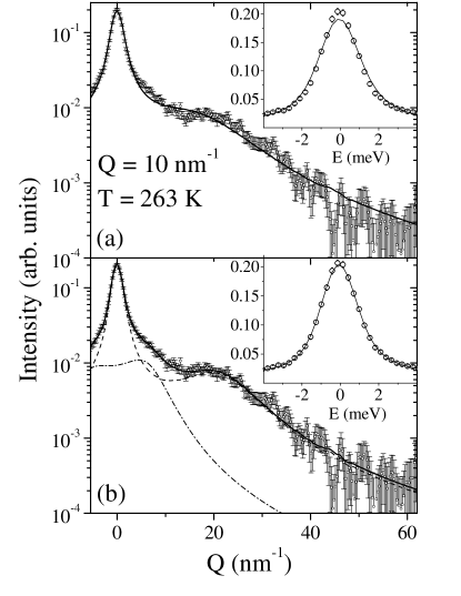
Figure 1: IXS spectrum at $Q$=10 nm^-1, T=263 K and P=2 kbar. The experimental data and their error bars are shown together with the best fits utilizing the model function described in the text with and without the second inelastic contribution. Panel (a): one viscoelastic contribution. Panel (b): one viscoelastic contribution and one damped harmonic oscillator model. The inset shows the central peak region.

The viscoelastic analysis of the water IXS spectra previously performed 10 was confined to $Q$-values not exceeding $Q$=7 nm^-1, a region in which the second excitation discussed in the introduction is not visible. Consequently, the applied theoretical formalism yielded excellent agreement between the model function and the experimental data. In the present case, the inclusion of a second excitation is mandatory as it is evident, for example, by inspection of Figure 1, which reports the IXS spectrum recorded at $T$=263 K, $P$=2 kbar and $Q$=10 nm^-1. In this figure, panel (a) shows the best fit to the data with only one excitation (viscoelastic model) according to Eq. 2. Both the inelastic and the central part of the spectra are not well reproduced, and it is obvious that a second excitation has to be added. This has been done for the fit presented in panel (b) where the second excitation is accounted for by a damped-harmonic oscillator (DHO) function 21 added to the viscoelastic $S(Q,\omega)$, resulting in a significantly better fit. It is important to stress that this is a purely empirical approach to introduce the mixing phenomenon of longitudinal and transverse dynamics. A correct theoretical description should provide a memory function, directly reproducing a double-excitation line shape, which naturally would involve a much larger set of variables. In particular, such a formalism should be extended to a regime of broken ergodicity, when the frequency range is much higher than the structural relaxation time ($\omega\tau_{\alpha}>1$). In this range the symmetry arguments that decouple the transverse (T) from the longitudinal (L) variables in the generalized Langevin equation must be abandoned and a coupling $L-T$ mechanism must be taken into account. Work along these lines is currently in progress. Within the present context, the choice of a DHO lineshape to describe the transverse dynamics is used empirically to provide information on the intensity and the frequency of the second excitation. In summary, the model function used to represent the spectra is composed of the following pieces:

1. A viscoelastic model function, proportional to Eq. 2, to account for the central peak and the longitudinal dynamics:

   $$s^{(L)}(Q,\omega)\;=\;\frac{A_{L}}{\pi}\frac{\omega_{0}^{2}\tilde{m}_{Q}^{\prime}(\omega)}{(\omega_{0}^{2}-\omega^{2}-\omega\tilde{m}_{Q}^{\prime\prime}(\omega))^{2}+(\omega\tilde{m}_{Q}^{\prime}(\omega))^{2}}$$

   We have neglected the contribution due to thermal relaxation, which amounts to set $\gamma(Q)=1$, an approximation which turns out to be very good in the high Q region.

2. A DHO line-shape for the second excitation:

   $$s^{(T)}(Q,\omega)\;=\;\frac{A_{T}}{\pi}\frac{\Omega_{T}^{2}\Gamma_{T}}{(\Omega^{2}_{T}-\omega^{2})^{2}+(\omega\Gamma_{T})^{2}}$$

   Where $\Omega_{T}$ is the maximum of the ”transverse-like” contribution to the the longitudinal current spectrum (the dynamic structure factor multiplied by $\omega^{2}/Q^{2}$, i. e. of $\omega^{2}s^{(T)}(Q,\omega)$) and $\Gamma_{T}$ is the width of the inelastic transverse peaks.

This model function for the dynamic structure factor is symmetric, and, in order to account for the quantized character of the energy transfers at the microscopic level, has to be weighted with a function that i) satisfies the detailed balance and ii) becomes unity in the classical limit ($\hbar\omega/K_{B}T<<1$). Among the possible choices, the weighting factor usually utilized is:

$$w(\omega,T)=\frac{\hbar\omega}{K_{B}T}(n(\omega,T)+1)=\frac{\hbar\omega}{K_{B}T}[1-exp(-\hbar\omega/k_{B}T)]^{-1}$$

Finally, the theoretical model has to be convoluted with the experimental resolution function $R(\omega)$, to give a fitting function of the form:

$$I(Q,\omega)\;=\;\{R(\omega)\}\;\otimes\;\{\frac{\hbar\omega}{K_{B}T}[n(\omega,T)+1][s^{(L)}(Q,\omega)+s^{(T)}(Q,\omega)]\}\;+\;B$$ (5)

Here B is an additional term which accounts for the electronic and environmental background of the detectors. As a result, the data are fitted with 9 free parameters: i) the background $B$; the transverse ii) ”intensity” $A_{T}$, iii) position $\Omega_{T}$ and iv) width $\Gamma_{T}$; v)the longitudinal intensity $A_{L}$; the three parameters of the longitudinal memory function, namely the structural relaxation vi) time $\tau_{\alpha}$ and vii) strength $\Delta$ and the area of the microscopic relaxation $\Gamma_{\mu}$; and, finally, ix) the static structure factor $S(Q)$ entering in the term $\omega_{o}$. All these parameters are, in principle, $T$- and $Q$-dependent.

As a matter of fact, $\Gamma_{\mu}$, which represents the topological microscopic disorder contribution to the acoustic attenuation, is known to have a negligible temperature dependence. Therefore we have fixed its value to the one obtained at the lowest temperature. We checked that leaving this parameter free does not change significatively the values of the other parameters. Moreover, we observe that, for the highest temperature spectra, leaving the energy position and width of the transverse contribution as free parameters in the fit, results in a meaningless overdamping of the DHO function to the extent that it cannot be distinguished from the purely relaxational elastic contribution already accounted for by the viscoelastic model (the intensity of this contribution vanishes at high $T$, thus implying that $\Omega_{T}$ and $\Gamma_{T}$ become irrelevant). In order to circumvent this, and guided by the observation of Sokolov et al. sok , the position and width of the second excitation was unambiguously determined in an unconstrained fit for the lowest temperature IXS spectra, and kept fixed at higher temperatures. Therefore, at all temperature but the lowest, there are six free fitting parameters.

II.3 Experimental results

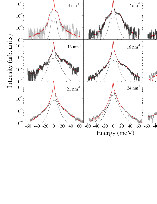
Figure 2: IXS spectra of water at $T$=263 K and $P$=2 kbar. The figure reports the data (dots) normalized to the total integrated intensity on a logarithmic scale emphasizing the inelastic part of the spectrum. The solid line represents the total fit result as explained in the text, while the other lines visualize the two contributions to the fitting model: the longitudinal and quasi-elastic one represented by a viscoelastic model (dashed line) and the transverse-like secondary peak accounted for by a DHO model function (dash-dotted line)

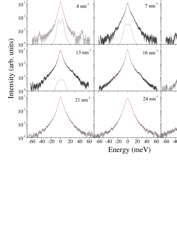
Figure 3: IXS spectra at $T$=419 K and $P$=95 bar. The figure reports the data (dots) normalized to the total integrated intensity on a logarithmic scale emphasizing the inelastic part of the spectrum. The solid line represents the fit result as explained in the text, while the other lines visualize the two contributions to the fitting model: the longitudinal and quasi-elastic one represented by a viscoelastic model (dashed line) and the transverse-like secondary peak accounted for by a DHO model function (dash-dotted line)

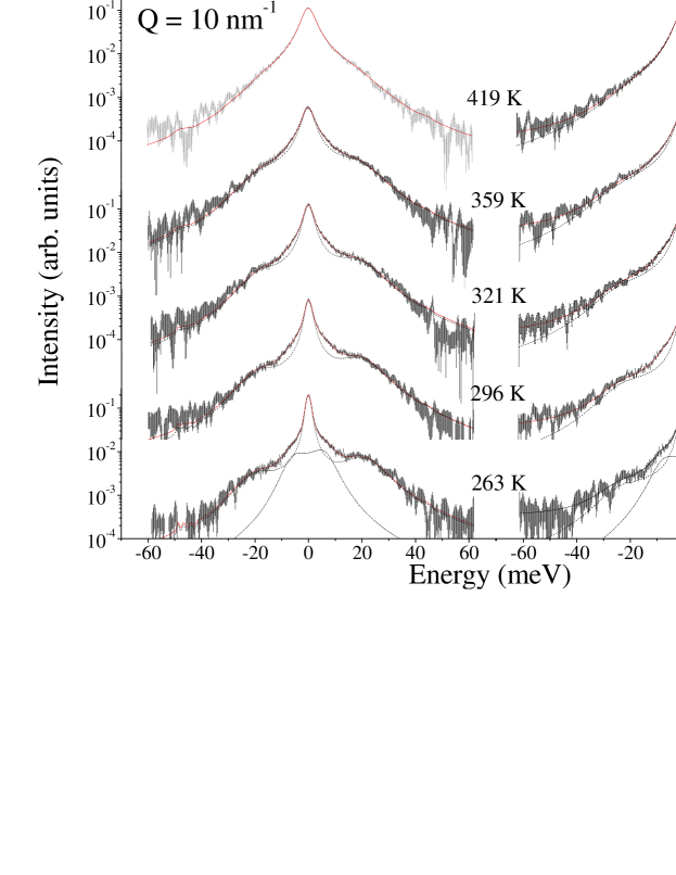
Figure 4: Temperature evolution of the IXS spectra for $Q$=10 $nm^{-1}$ (left panel) and $Q$ = 13 $nm^{-1}$ (right panel). The figure reports the data (dots) normalized to the total integrated intensity on a logarithmic scale emphasizing the inelastic part of the spectrum. The solid line represents the fit result as explained in the text, while the other lines visualize the two contributions to the fitting model: the longitudinal and quasi-elastic one represented by a viscoelastic model (dashed line) and the transverse-like secondary peak accounted for by a DHO model function (dash-dotted line).

IXS spectra were recorded at the different temperatures and pressures as indicated in Table 1, spanning the momentum transfer, Q, region from 4 to 16 nm^-1 with an approximate constant spacing of 3 nm^-1. For the lowest (263 K) and highest (419 K) temperatures, the Q-range was extended to 30 nm^-1. The spectra extend up to 60 meV on both sides of the elastic line, with an integration time of 100 s per spectrum. For each setting three spectra were collected, and subsequently summed in order to achieve the high statistical accuracy required for the data analysis. Typical total counts range between 1500 (at 4 nm^-1), 2500 (at 9.93 nm^-1), and 3500 (at 12.91 nm^-1). To account for the slow drift of the photon flux impinging on the sample, the collected data were normalized to the intensity of the incident beam. A typical IXS spectrum is shown on a logarithmic scale in figure 1. The experimental data with their error bars are shown together with the best fits (full lines) using both the model function discussed before (bottom panel) and the same function with $A_{T}$=0 (top panel). For clarity, only the elastic and the Stokes part of the spectrum is shown. The insets provide a zoom of the elastic line region on a linear scale. It can be easily appreciated that a fit using a viscoelastic model only (top panel), does not properly describe the IXS data, leading to a poor fit of both the elastic line and the inelastic part of the spectrum (the reduced $\chi^{2}$ results to be $\approx$ 2, i. e. more than 10$\sigma_{\chi^{2}}$ larger than its expected value). The inclusion of a second inelastic excitation significantly improves the quality of the fit (reduced $\chi^{2}\approx 1$, $\sigma_{\chi^{2}}\approx 0.1$), as can be seen in the lower panel. For all fitted spectra, the value of $\chi^{2}$ remained within one standard deviation from the expected value.

Figure 2 shows as an example the $Q$ evolution of the IXS data recorded at T=263 K and P=2000 bar. The two inelastic contributions which clearly appear at $Q$=10 nm^-1 can also be seen throughout the whole Q-range. As can be noticed by the $Q$ evolution of the dashed and dotted lines (longitudinal and transverse-like contributions, respectively) the intensity of the low-frequency (transverse-like) mode increases with increasing $Q$.

The shape of the IXS spectra as well as their $Q$-dependence is markedly different at $T$=419 K and $P$=95 bar (see figure 3). The elastic line appears broader, and consequently the low frequency, non dispersing mode is much less visible. As a matter of fact, it can only be identified in the spectra with $Q$ $\leq$ 13 nm^-1, while for larger Q values the increasing width of the elastic line completely governs the spectral shape. The weak feature at about 45 meV in the spectra at $Q$=4 nm^-1 is the contribution from the high-pressure cell windows and corresponds to the diamond longitudinal acoustic phonon.

To show an example of the temperature evolution of the IXS spectra, and more specifically, of the behavior of the second weakly dispersing feature, the spectra recorded at $Q$=10 (left panel) and 13 nm^-1 (right panel) are shown in figure 4 at the indicated temperatures. At the lowest temperature, the experimental data are shown together with the best fit to the model function and the two individual components (viscoelastic model and DHO). For the higher temperatures, only the viscoelastic contribution and the total fit are shown for the sake of clarity and in order to emphasize the decreasing importance of the second excitation. We notice a clear trend for both momentum transfers: with increasing temperature the contribution of the second excitation becomes smaller and smaller to the extent that it completely disappears at the highest temperature.

III Data analysis and discussion

III.1 The longitudinal dynamics

Figure 5: $Q$-dependence of the (scaled) structural relaxation time $\tau_{\alpha}^{\star}=\tau_{\alpha}\times\eta(T=263K)/\eta(T)$ (see text). The dashed line reports the fit results of 10 for the Q dependence of the relaxation time at $T=263K$, valid up to Q = 7 $nm^{-1}$.

Figure 6: Temperature evolution of the structural relaxation time (full symbols) at different $Q$-values between 7 and 16 $nm^{-1}$. The shear viscosity $\eta(T)$ is reported for comparison (open dots), as well as the $Q=0$ extrapolation of the relaxation time 10 (solid line).

In the present section we present and discuss the results obtained for the longitudinal dynamics which are retrieved from the viscoelastic analysis as described in detail in section II B.

In figure 5 we report the $Q$-dependence of the structural relaxation time $\tau_{\alpha}$ at different temperatures $T$, scaled by the shear viscosity ratio $r(T)=\eta(T=263K)/\eta(T)$: i. e. $\tau_{\alpha}^{\star}$ = $r(T)\tau_{\alpha}(T)$. This scaling has been performed in order to verify whether the structural relaxation time is proportional to the longitudinal viscosity $\eta$, a relationship which generally holds in the continuum limit $Q\longrightarrow 0$. It is evident from the inspection of figure 5 that the $Q$ evolution of $\tau_{\alpha}$ at different T is indeed the same, especially in the $Q$-range below 20 nm^-1. As implied by the validity of the scaling, the $T$ and the $Q$ dependence of the relaxation time can be factorized: $\tau_{\alpha}(Q,T)=\eta(T)f(Q)$, being $f(Q)$ the function that describes the $Q$-evolution of the relaxation time. The dashed line at low $Q$ in Fig. 5 reports the dependence of the relaxation time for $T$=263 K, derived in Ref. 10 ; it turns out to be consistent with the present results. Figure 6 shows the temperature dependence of $\tau_{\alpha}$ for different $Q$-values between 7 and 16 nm^-1. The evolution of the viscosity (open circles) and the $Q\rightarrow 0$ limit of $\tau_{\alpha}(Q,T)$ (solid line) as reported in Ref. 10 are also shown. The good overall agreement confirms the reliability of the structural relaxation time determination by the viscoelastic model over the large $Q$ range and in the different thermodynamic conditions investigated here.

The temperature dependence of the zero frequency sound velocity ($c_{0}=\omega_{0}/Q$), the infinite frequency sound velocity ($c_{\infty}=\sqrt{(\Delta^{2}+\omega_{0}^{2})}/Q$) and the apparent sound velocity ($c_{L}=\Omega_{L}/Q$) are reported in figure 7 for $T$=263 K (left panel) and $T$=419 K (right panel). Here, $\Omega_{L}$ is the maximum of the function $\omega^{2}s^{(L)}(Q,\omega)$ calculated using the best fit parameters. The bottom panels of Fig. 7 show the $Q$-dependence of the product $\Omega_{L}\tau_{\alpha}$, the parameter that indicates whether the dynamics is viscous-like ($\Omega_{L}\tau_{\alpha}<1$) or elastic-like ($\Omega_{L}\tau_{\alpha}>1$). For $T$=263 K, $\Omega_{L}\tau_{\alpha}$ is always larger than, or close to, one, the system has a solid-like response, and the sound velocity $c_{L}$ is close to $c_{\infty}$, its infinite frequency value, over the whole explored $Q$-range. In contrast, at $T$=419 K, $\Omega_{L}\tau_{\alpha}$ is larger than one only over a limited $Q$-range, from 4 to 10 nm^-1, and then decreases rapidly below one for increasing $Q$-values. Consequently, we observe a transition from the infinite- to the zero-frequency sound regime: it takes place for $Q$ values between 10 and 15 nm^-1. This is the first experimental observation of the transition $c_{\infty}\rightarrow c_{0}$ that takes place for $Q$-values around the $Q$’s where the $S(Q)$ shows its first maximum, as a consequence of the De Gennes narrowing.The $Q$ dependence of the excitation frequency, in fact, shows a decrease with a minimum just in correspondence with the first maximum of the $S(Q)$ as a memory of a ”pseudo-Second Brillouin zone”. At the same time the relaxation time decreases towards high $Q$ with respect to the $Q=0$ value with a slight increase at around 27 nm^-1 again due to De Gennes narrowing (see figure 5). Such kind of $c_{\infty}\rightarrow c_{0}$ transition, taking place at $Q$ values around the first maximum of the $S(Q)$, has been already observed in MD simulations of a Lennard-Jones model glass nonh . Furthermore, we note that our derived values for $c_{0}$ is in excellent agreement with independent determinations, both in the limit of $Q\rightarrow 0$ and at high $Q$-values. The values of $c_{0}$ in the low $Q$-limit were obtained from thermodynamic data 16 , and are indicated by the arrows in Fig. 7. The zero frequency sound velocity in the high-$Q$ region (dash-dotted line) has been calculated utilizing the expression for $c_{0}(Q)$ within the framework of generalized hydrodynamics:

$$c_{0}=\sqrt{\frac{K_{B}T}{MS(Q)}}$$ (6)

Here, we utilized the $S(Q)$ values determined by neutron diffraction measurements ricci at the same thermodynamical conditions (the $S_{OO}$ partial structure factor has been used). The agreement of $c_{0}(Q)$, calculated using the previous relation, and $c_{0}(Q)$ derived from the fits convincingly demonstrates the solidity of our data analysis procedure.

As expected for a viscoelastic behavior of the excitation, the same $c_{0}\leftrightarrows c_{\infty}$ transition can be observed at fixed $Q$ due to the effect of the temperature on $\tau_{\alpha}$. Figure 8 shows $c_{L}$, $c_{0}$ and $c_{\infty}$ as a function of temperature for $Q$=16 nm^-1. At low $T$ the relaxation time is long, $\Omega_{L}\tau_{\alpha}>>1$, and the apparent sound velocity is close to $c_{\infty}$. When, on increasing the temperature, the structural relaxation enters in the excitation timescale ($\Omega_{L}\tau_{\alpha}\approx 1$), the sound velocity $c_{L}$ recovers its liquid-like value $c_{0}$.

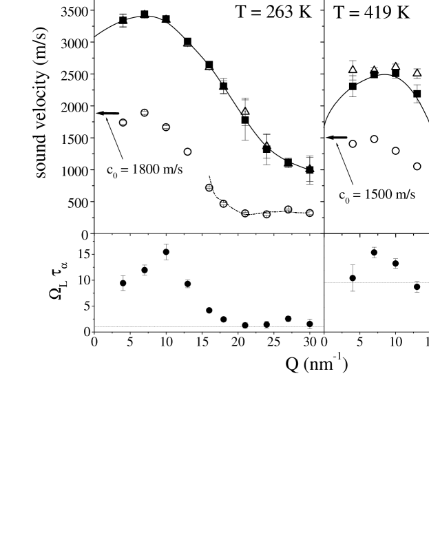
Figure 7: Sound velocities and the product $\Omega_{L}\tau_{\alpha}$ -as determined by the fit to the IXS spectra- as a function of $Q$, and at two different temperatures: $T$=263 K (left panels) and $T$=419 K (right panels). The top panels show the $Q$-evolution of the sound velocities $c_{0}$ (open dots), $c_{\infty}$ (open triangles), and $c_{L}$ (full squares), whereas the bottom panels show the product $\Omega_{L}\tau_{\alpha}$, that, when equal to unity, marks the transition from the infinite frequency sound velocity $c_{\infty}$ to the zero-frequency sound velocity $c_{0}$. The solid line is a guide to the eye. The hydrodynamic ($Q$=0) value of $c_{0}$ is indicated by arrows; the Q-evolution of $c_{0}(Q)$, as derived using Eq. 6 and the $S(Q)$ determined by neutron scattering, is indicated by the dash-dotted line in the $Q$ region where neutron data are available. The dotted horizontal line in the lower panels marks the condition $\Omega_{L}\tau_{\alpha}$ = 1.

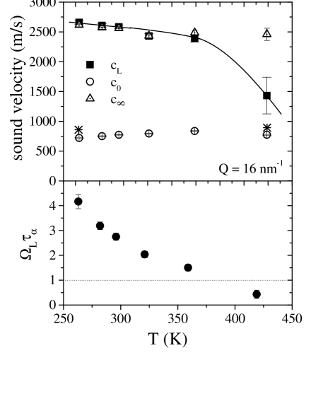
Figure 8: The temperature dependence of the sound velocities and of the product $\Omega_{L}\tau_{\alpha}$ for $Q$=16 nm^-1. The data show the same phenomenology as those reported in fig. 7. Here the product $\Omega_{L}\tau_{\alpha}$ is changed by varying the relaxation time scale: as in the previous case we start to observe the transition when we approach $\Omega_{L}\tau_{\alpha}\approx 1$. The solid line is a guide to the eye. The stars in the upper panel indicate the $c_{0}(Q)$ values as derived from Eq. 6 for the thermodynamical points available from the neutron diffraction database ricci .

III.2 The second excitation

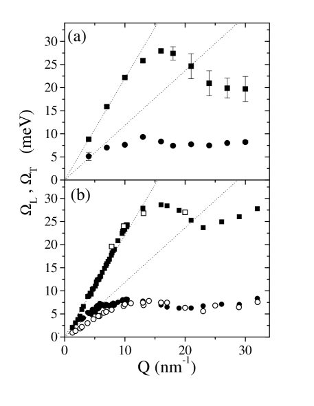
Figure 9: Panel (a): Longitudinal current peaks positions from the fits of IXS data of liquid water at T=263 K and P=2 kbar. Panel (b): MD simulations results 22 (see text). The dotted lines represent excitations with a linear dispersion in Q, corresponding to a sound speed of 3300 and 1900 m/s, respectively.

As already discussed in some detail above, the IXS spectra, especially at low temperature, can only be properly described if one takes into account a second inelastic excitation. This second excitation is described by three parameters (intensity, peak position and peak width). Figure 9 shows the dispersion ($Q$-dependence) of $\Omega_{T}$, together with that of $\Omega_{L}$, at T=263 K and P=2000 bar, where the second excitation is best appreciated. The upper panel shows the result of the present work. The longitudinal frequency $\Omega_{L}$ (squares) and the ”transverse” frequency $\Omega_{T}$ (circles) (both derived from the fit procedure) show the expected behavior: a linear dispersion followed by a bend down and a minimum in the $Q$ region where $S(Q)$ has its maximum for the longitudinal excitation, and a weak $Q$ dependence for the transverse mode. Full symbols in the lower panel correspond to the results of a previous MD simulation 22 for the position of the Longitudinal current peaks. These were carried out considering 4000 $D_{2}O$ molecules enclosed in a cubic box with periodic boundary conditions, and utilizing the SPC/E model 23 . The simulations were performed at a density of 1 g/cm³ and T $\approx$ 250 K. The qualitative agreement between experiment and simulation is remarkable. We note slight differences in the absolute values of the excitation energies: while the maximum of the longitudinal dispersion is slightly lower, the energies for the second excitation are slightly higher in the case of the IXS results. Moreover a small displacement at higher $Q$ in the position of the first minimum in the IXS data is justified as these are taken at high pressure while the simulations are performed at ambient conditions: as the pressure doesn’t affect very much the value of $c_{\infty}$ the agreement with the simulation data in the linear region is extremely good. The open symbols, also reported in the lower panel, indicate for some $Q$ values the position of the two peaks found in the Transverse Current spectra, a quantity that is not experimentally observable, but that can be determined by MD simulations. The position of these peaks clearly coincides with the correspondent peak measured in the Longitudinal Current, supporting the presence of a mixing phenomenon 22 . We further note that the energy range over which the weakly dispersing feature is observed corresponds to the TA / TO branch in hexagonal ice as determined by INS 24 and IXS 25 .

To further characterize the second excitation we now study its integrated intensity. Specifically, in figure 10 we report the ”transverse” intensity $A_{T}$ normalized to the total integrated intensity $A_{T}+A_{L}$ as a function of $Q$ for the selected thermodynamic point $T$=263 K and $P$=2 kbar. In the lower panel of Fig. 10, we report the evolution of $\Omega_{T}\tau_{\alpha}$. We observe a general increasing trend of the parameter $A_{T}/(A_{T}+A_{L})$ with increasing $Q$. It is worth to observe that the appearance of a transverse-like contribution with an intensity increasing with $Q$ has also been registered in experiments and simulations on glassy systems as glycerol gly and silica sio2a ; sio2b ; sio2c . In silica the mixing phenomenon turns out to be particularly enhanced both in MD simulation and experiments indicating that, as in water, the local tetrahedral structure favors the coupling of the L and T dynamics. The intensity increase with $Q$ is expected on the basis of a simple one-excitation picture within the harmonic approximation for the dynamic structure factor, suggesting that, for a non-dispersive excitation, $A_{T}/(A_{T}+A_{L})\approx Q^{2}$. More importantly, we also observe that, superimposed to the growth of $A_{T}/(A_{T}+A_{L})$ with $Q$, there is also a ”modulation” in phase with $\Omega_{T}\tau_{\alpha}$. When, at $Q\approx$ 15 nm^-1, $\Omega_{T}\tau_{\alpha}$ become less than unity, the intensity of the ”transverse” peak decreases.

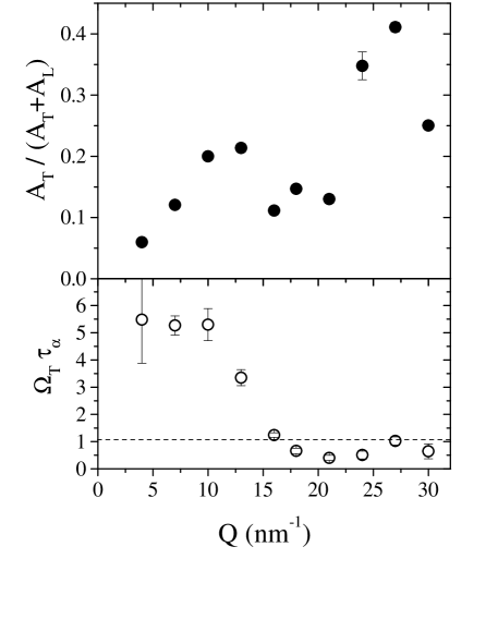
Figure 10: $Q$-dependence of the transverse to total integrated intensity ratio (upper panel) and the product $\Omega_{T}\tau_{\alpha}$ (lower panel) at T=263K. The dashed horizontal line indicates the condition $\Omega_{T}\tau_{\alpha}$ = 1.

The presence of a strong correlation between the intensity of the transverse peak and the $\Omega_{T}\tau_{\alpha}$ is confirmed by inspecting their temperature evolution reported in figure 11 for two selected $Q$ values: $Q$ =10 and 13 nm^-1. Here, when the time scale of the $\alpha$-relaxation is comparable to the inverse of the frequency of the transverse excitation, the ratio $A_{T}/(A_{T}+A_{L})$ decreases, and for the highest temperature becomes essentially zero. This behavior -very different from that of the longitudinal collective mode, which is affected by the relaxation only in the sound velocity value- is just the one expected for a transverse-like excitation: recovering a liquid-like regime the system is no longer able to give an elastic response to a shear stress and to sustain propagating transverse waves. In this regime the transverse dynamics assumes a purely relaxational behavior, corresponding to a peak at $\omega=0$ in the current spectrum 17 . For this reason, still lacking a formal model for the coupling, the fits at higher temperatures have been performed just fixing the DHO parameters at the lowest T values leaving the intensity $A_{T}$ free. This procedure allows us to provide the information on the inelastic contribution of the dispersion-less mode leaving the relaxational behavior accounted for by the viscoelastic model. This procedure, as can be seen by bare eye in the spectra at high T, doesn’t affect at all the statistical significance of the fits also when the transverse-like contribution, which was mandatory at low T, can be completely neglected.

Figure 11: Top panels: temperature evolution of the transverse to total integrated intensity ratio $A_{T}/(A_{T}+A_{L})$ at momentum transfers of 10 $nm^{-1}$ (left panel) and 13 $nm^{-1}$ (right panel). The solid lines are guides to the eye. Bottom panels: temperature evolution of $\Omega_{T}\tau_{\alpha}$. The dotted horizontal line marks the condition $\Omega_{T}\tau_{\alpha}$ = 1.

IV Conclusions

In this paper the viscoelastic analysis of the IXS spectra of water, already successfully performed in the low $Q$ range, has been extended to much larger $Q$ values and in a wide range of thermodynamical conditions.

At the high $Q$ values investigated here the presence of a second excitation in the spectra cannot anymore be neglected and it has been successfully taken into account in the analysis revealing a behavior in agreement with the viscoelastic expectation for a transverse-like excitation. This findings confirm our assignment of a transverse nature to the dispersion-less mode of water observed at an energy of $\approx$ 6 meV.

Furthermore the large variations of the structural relaxation time (almost a decade) in the investigated thermodynamic range has allowed us to perform an excellent test of the viscoelastic picture. Summarizing, the two main results of the present work are:

1. The longitudinal-like dynamics can be properly accounted for by a viscoelastic model also in the high $Q$ range: indeed, besides the now well known transition from $c_{O}$ to $c_{\infty}$ that takes place at small $Q$ ($Q\approx$ 4 nm^-1 at ambient conditions), for the first time the transition from $c_{\infty}$ back to $c_{0}$, taking place at high Q values, could be observed. This back-transition is a consequence of the De-Gennes narrowing on the product $\Omega_{L}\tau_{\alpha}$ that becomes smaller than one at $Q$ values around the $Q$’s of the main peak in the $S(Q)$.

2. The second dispersion-less mode behaves as a transverse-like excitation disappearing from the spectra as soon as the structural relaxation process reaches the excitation time scale ($\Omega_{T}\tau_{\alpha}$ = 1)

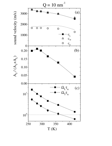
Figure 12: Comparison of the temperature evolution of the L-like and T-like dynamics for a fixed $Q$ value ($Q$= 10 $nm^{-1}$). (a) Evolution of the three velocities as in figure 8; the dashed line corresponds to the thermodynamic prediction for $c_{0}$. (b) Temperature evolution of the transverse to total integrated intensity ratio $A_{T}/(A_{T}+A_{L})$. (c) Temperature evolution of $\Omega_{T}\tau_{\alpha}$ and $\Omega_{L}\tau_{\alpha}$; the dotted horizontal line marks the condition $\Omega\tau_{\alpha}$ = 1 clearly showing that the two dynamics are in different regimes at high $T$. The solid lines are guides to the eye.

Finally, a few words must be devoted to the comparison between the present -viscoelastic- explanation of the high frequency dynamics of water and the alternative -solid based- description as discussed in the introduction. To this purpose we compare in figure 12 the temperature behavior of the longitudinal and transverse dynamics for a fixed $Q$ value ($Q$=10 nm^-1). In panel (a) we report the velocities plot as in figure 8 (here for a different $Q$ value) while in panel (b) we report the (normalized) intensity of the dispersion-less mode at the same $Q$ value. The comparison of the two uppermost panels in figure 12 clearly demonstrates that while the apparent sound velocity ($c_{L}$, full squares in panel (a)) is still far from from $c_{0}$ (open dots) -i. e. the system is in the elastic limit over the whole $T$ range-, the intensity of the second excitation becomes negligible at high $T$. Thus we have that, at high $T$ the system is in the elastic regime, but the second excitation can no longer be appreciated in the spectra. This evidence cannot be framed in the interaction model proposed in Ref. 8 ; sacchnew that traces the ”fast sound” phenomenon back to the presence and the interaction between two modes. This observation, however, has a clear explanation in the viscoelastic picture as illustrated in panel (c). While the structural relaxation process has already reached the transverse-like mode time scales, with $\Omega_{T}\tau_{\alpha}<$ 1 for $T>$ 370 K thus entering the viscous regime, it is still not affecting the higher energy longitudinal-like excitation which still exhibits an elastic response ($\Omega_{L}\tau_{\alpha}>$ 1 up to the highest explored temperature).

The data reported in Fig. 12, together with the outcome listed in items (1) and (2) before, are the main results of this paper. All these results favor the viscoelastic description of the high frequency dynamics of water. As a final observation, it must be noted that the two models discussed before are not so different as it appears at a first glance: in both cases it is the interaction of the sound waves with another ”mode” which causes both the positive dispersion of the apparent sound velocity and the appearance of a second peak in the dynamic structure factor. In the viscoelastic case the second mode is purely relaxing, in the solid-like approaches the second modes have a propagating component. However, major differences arise in interpreting the physical meaning of the parameters entering in the models: i) in the solid-like model no information of the structural relaxation time is contained, while $\tau_{\alpha}$ is directly measurable in the viscoelastic model, it is in agreement with independent determinations 9c ; 10 , and its values allow to calculate the viscosity, again in agreement with independent measurements 10 ; ii) A further evidence, again in the same direction, comes from the temperature dependence of the energy of the second mode. In the solid-like framework, at increasing temperature the data indicate a decrease of the interaction parameter, corresponding to a decrease of the energy position of the dispersion-less mode. This decrease of the energy of the dispersion-less mode is not observed; for example, the depolarized light scattering measurements sok do not show any noticeable shift in the position of the peak that corresponds to the density of states of the second excitation; iii) Finally, let us observe that the viscoelastic-based explanation of the dynamics of the density fluctuations is actually considered the proper approach in many liquids viscoOK and it has been substantiated by rigorous theories as the Mode Coupling Theory MCT (a theory that, via MD, has been proved to work properly also in liquid water MCT_water ). In other words, as the dynamic of liquid water shows the same phenomenology of that of many other liquids, why, in water, should one look for a different explanation?

V Acknowledgment

We thank M. A. Ricci for pointing out the neutron diffraction database ricci .

References

- (1) C.A. Angell, in Water: A comprehensive Treatise, edited by F. Franks (Plenum, New York, 1981), Vol. 7.
- (2) P.G. Debenedetti,Metastable Liquids (Princeton University Press, 1996).
- (3) C. Roenne, L. Thrane, P.-O. Astrand, A. Wallqvist, K.V. Mikkelsen, and S.R. Keiding, J. Chem. Phys. 107, 5319 (1997).
- (4) R. Torre, P. Bartolini, R. Righini, Nature 428, 296(2004)
- (5) L. van Hove, Phys. Rev. 95, 249 (1954).
- (6) P. Bosi, F. Dupre’, F. Menzinger, F. Sacchetti, and M. C. Spinelli, Nuovo Cimento Lett. 21, 436 (1978).
- (7) J. Teixeira, M.-C. Bellissent-Funel, S.H. Chen, and B. Dorner, Phys. Rev. Lett. 54, 2681 (1985).
- (8) F.J. Bermejo, M. Alvarez, S.M. Bennington, and R. Vallauri, Phys. Rev. E 51, 2250 (1995).
- (9) C. Petrillo, F. Sacchetti, B. Dorner, and J.-B. Suck, Phys. Rev. E 62, 3611 (2000).
- (10) F. Sacchetti, J.-B. Suck, C. Petrillo, and B. Dorner, Phys. Rev. E 69, 061203 (2004).
- (11) F. Sette, G. Ruocco, M. Krisch, U. Bergmann, C. Masciovecchio, V. Mazzacurati, G. Signorelli, and R. Verbeni. Phys. Rev. Lett. 75, 850 (1995).
- (12) G. Ruocco, F. Sette, M. Krisch, U. Bergmann, C. Masciovecchio, V. Mazzacurati, G. Signorelli, and R. Verbeni. Nature 379, 521 (1996).
- (13) F. Sette, G. Ruocco, M. Krisch, C. Masciovecchio, R. Verbeni, and U. Bergmann, Phys. Rev. Lett. 77, 83 (1996).
- (14) A. Cunsolo, G. Ruocco, F. Sette, C. Masciovecchio, A. Mermet, G. Monaco, M. Sampoli, and R. Verbeni. Phys. Rev. Lett. 82, 775 (1999).
- (15) G. Monaco, A. Cunsolo, G. Ruocco, and F, Sette, Phys. Rev. E 60, 5505 (1999).
- (16) G. Ruocco and F. Sette, J.Phys.: Cond. Matt. 11, R259 (1999).
- (17) M. Krisch et al., Phys. Rev. Lett. 89, 125502 (2002).
- (18) M. Sampoli, G. Ruocco, and F. Sette, Phys. Rev. Lett. 79, 1678 (1997).
- (19) It is worth to point out that this is not different from what proposed in 25 as the optic modes supported by Petrillo et al. 8 is the gap-less prosecution of the TA mode in an extended BZ zone description of the phonon-like dynamics.
- (20) EURISYS Mesures, Lingolsheim, France.
- (21) A. Saul and W. Wagner, J. Phys. Chem. Ref. Data 18, 1537 (1989).
- (22) J.P. Boon and S. Yip, Molecular Hydrodynamics (Dover, New York, 1991).
- (23) U. Balucani and M. Zoppi, Dynamics of the Liquid State (MacGraw-Hill, New York, 1980).
- (24) A. Cunsolo, G. Pratesi, R. Verbeni, D. Colognesi, G. Monaco, C. Masciovecchio, G. Ruocco, and F. Sette, J. Chem. Phys. 114, 2259 (2001).
- (25) T. Scopigno, F. Sette, G. Ruocco, and G. Viliani, Phys. Rev. E66, 031205 (2002).
- (26) G. Monaco, D. Fioretto, L. Comez, and G. Ruocco, Phys. Rev. E63, 061502 (2001).
- (27) G. Ruocco, and F. Sette, J. of Phys.: Cond. Matt. 13, 9141 (2001).
- (28) G. Harrison, The Dynamical Properties of Supercooled Liquids (Academic Press, New York, 1976).
- (29) C. Masciovecchio, S. C. Santucci, A. Gessini, S. Di Fonzo, G. Ruocco, and F. Sette, Phys. Rev. Lett. 92, 255507 (2004).
- (30) B. Fak and B. Dorner, Institut Laue Langevin (Grenoble, France), technical report No. 92FA008S, (1992).
- (31) G. Ruocco, F. Sette, R. Di Leonardo, G. Monaco, M. Sampoli, T. Scopigno, and G. Viliani, Phys. Rev. Lett. 84, 5788 (2000).
- (32) http://www.isis.rl.ac.uk/disordered/Database/DBMain.htm
- (33) H.J.C. Berendsen, J.P.M. Postma, W.F. Van Gunsteren, and H.J. Hermans, in Intermolecular Forces, edited by B. Pulman (Reidel, Dordrecht, 1981), p. 331.
- (34) B. Renker, Phys. Lett. A 30, 493 (1969).
- (35) T. Scopigno, E. Pontecorvo, R. Di Leonardo, M. Krisch, G. Monaco, G. Ruocco, B. Ruzicka, and F. Sette. Journal of Physics Condensed Matter 15, S1269 (2003).
- (36) R. Dell’Anna, G. Ruocco, M. Sampoli, and G. Viliani, Phys. Rev. Lett. 80, 1236 (1998).
- (37) B. Ruzicka, T. Scopigno, S. Caponi, A. Fontana, O. Pilla, P. Giura, G. Monaco, E. Pontecorvo, G. Ruocco, F. Sette. Physical Review B 69, 100201R (2004).
- (38) A. P. Sokolov, J. Hurst and D. Quitmann, Phys. Rev. B 51, 12865 (1995).
- (39) See for example: Journal of Physics: Condensed Matter 15, S737-1290, ”Proceedings of the Third Workshop on Non-equilibrium Phenomena in Supercooled Fluids, Glasses and Amorphous Materials” (2003).
- (40) W. Goetze, L. Sjogren, Rep. Prog. Phys. 55, 241 (1992); W. Goetze, J. Phys.: Cond. Matt. 11, A1, (1999); H. .Z. Cummins, J. Phys.: Cond. Matt. 11, A95, (1999).
- (41) P. Gallo, F. Sciortino, P. Tartaglia, and S. H. Chen, Phys. Rev. Lett. 76, 2730 (1996); F. Sciortino, P. Gallo, P. Tartaglia, and S. H. Chen, Phys Rev. E 54, 6331 (1996); S. H. Chen, P. Gallo, F. Sciortino, and P. Tartaglia, Phys Rev. E 56, 4321 (1996); F.W. Starr, M.-C. Bellissent-Funel, and H. E. Stanley, Phys. Rev. Lett. 82, 3629 (1999); F. W. Starr, F. Sciortino, and H. E. Stanley, Phys. Rev. E 60, 6757 (1999); L. Fabbian, A. Latz, R. Schilling, F. Sciortino, P. Tartaglia and C. Theis, Phys. Rev. E 60, 5768 (1999).