Functional Renormalization for pinned elastic systems away from their steady states

Abstract

Using one loop functional RG we study two problems of pinned elastic systems away from their equilibrium or steady states. The critical regime of the depinning transition is investigated starting from a flat initial condition. It exhibits non trivial two-time dynamical regimes with exponents and scaling functions obtained in a dimensional expansion. The aging and equilibrium dynamics of the super-rough glass phase of the random Sine-Gordon model at low temperature is found to be characterized by a single dynamical exponent $z\approx c/T$, where $c$ compares well with recent numerical work. This agrees with the thermal boundary layer picture of pinned systems.

Disordered elastic systems offer many experimental realizations and are also of theoretical interest as prototype models for glasses induced by quenched disorder. The competition between the structural order and substrate impurities results in pinning, complex ground states, barriers and ultra slow glassy dynamics. While ground state, equilibrium dynamics, and driven steady state properties have been much studied theoretically, much less is known about the dynamics before the steady state is reached, or about the aging dynamics. If universality is shown there, it would be of high interest for numerous experimental systems, e.g. magnetic domain wall relaxation creepexp , superconductors vortices , contact line depinning rolley , density waves cdw .

Numerical studies of glassy dynamics are hampered by high barriers in configuration space resulting in ultra-long time scales making comparison with theory uncertain. In some cases however faster, but still interesting dynamics occurs. One is zero temperature $T=0$ driven dynamics near the depinning transition where barriers disappear frgdep1 . Recent theoretical progress has been achieved there. Functional renormalization group (FRG) studies give more precise and consistent predictions frgdep2 , corroborated by powerful new algorithms which allow for excellent determination of steady state exponents rosso ; allemands . One aim of this paper is to extend the FRG to dynamics away from steady states, and to show that interesting universal two-time dynamics (analogous to the aging dynamics in non driven situations) also occurs near depinning. We predict new exponents and scaling functions in the critical regime.

A second case where $T>0$ dynamics has been investigated is the ”marginal glass” phase exhibited by topologically ordered 2D periodic systems as captured by the Cardy Ostlund (CO) model co . Barriers there grow only logarithmically with size allowing for precise numerics simu_tc . The equilibrium tsai_super_rough and aging schehr_co_pre dynamics were studied using Coulomb gas RG methods, but only near the glass transition temperature $T_{g}$ toner . A numerical study has confirmed some of the RG predictions, and in addition has explored the full temperature regime schehr_co_num . The dynamical exponent was found to diverge as $z\sim 1/T$ at low $T$. One aim of this paper is to show this result within a simple one loop FRG, and to obtain detailed predictions for the aging regimes at low $T$. This study, together with the rather good agreement with numerics, is also important as indirect evidence for a recent hypothesis that a ”thermal boundary layer” (TBL) in the field theory controls the activated dynamics of (more strongly) pinned manifolds balentspld .

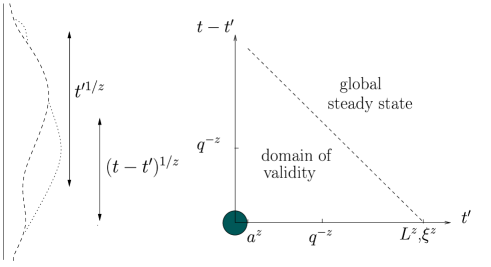
Figure 1: (a) solid line: initial flat configuration, dashed and dotted lines: configurations of the string at time $t^{\prime}$ and $t$ respectively. (b) Domain of validity, in logarithmic scale, of our approach near the depinning transition. The grey circle represents the small time region sensitive to microscopic details.

The overdamped dynamics of a single component elastic manifold of internal dimension $d$, parametrized by a height field $u(x,t)\equiv u_{xt}$ is described by

$$\eta\partial_{t}u_{x,t}=c\nabla^{2}u_{x,t}+F(x,u_{x,t}+vt)+f-\eta v+\xi(x,t)$$ (1)

where $\overline{u_{xt}}=0$, $\langle\xi(x,t)\xi(x^{\prime},t^{\prime})\rangle=2T\eta\delta^{d}(x-x^{\prime})\delta(t-t^{\prime})$ is the correlator of the thermal gaussian noise, $\overline{F(x,u)F(x^{\prime},u^{\prime})}=\Delta(u-u^{\prime})\delta^{d}(x-x^{\prime})$ the second cumulant of the quenched random pinning force and $v$ is the average velocity. We denote the small scale cutoff size $a\sim\Lambda_{0}^{-1}$. In this paper we consider a flat initial configuration $u_{xt=0}=0$. Denoting $u_{qt}$ the spatial Fourier transform of $u_{x,t}$, we focus on the correlation ${\cal C}^{q}_{tt^{\prime}}$ and the connected (w.r.t. the thermal fluctuations) correlation ${\tilde{\cal C}}^{q}_{tt^{\prime}}$:

$${\cal{C}}^{q}_{tt^{\prime}}=\overline{\langle{u}_{qt}{u}_{-qt^{\prime}}\rangle}\quad,\quad{\tilde{\cal C}}^{q}_{tt^{\prime}}=\overline{\langle{u}_{qt}{u}_{-qt^{\prime}}\rangle}-\overline{{\langle{u}_{qt}\rangle}{\langle{u}_{-qt^{\prime}}\rangle}}$$ (2)

and the response ${\cal R}^{q}_{tt^{\prime}}$ to a small external field ${h}_{-qt^{\prime}}$

$${\cal R}^{q}_{tt^{\prime}}=\overline{\delta\langle{u}_{qt}\rangle/\delta{h}_{-qt^{\prime}}}\quad,\quad t>t^{\prime}$$ (3)

where $\overline{..}$ and $\langle..\rangle$ denote respectively averages w.r.t. disorder and thermal fluctuations. In the following $R^{q}_{tt^{\prime}}=\eta^{-1}e^{-q^{2}(t-t^{\prime})/\eta}$ (respectively $C^{q}_{tt^{\prime}}$) denote the bare response function (respectively correlation), i.e. in the absence of disorder. We now specify the time regime $t,t^{\prime}$.

In the first situation studied below, i.e. an interface very near the depinning threshold, we set $T=0$ in (1). Numerical simulations of a manifold of internal size $L$ are typically performed on a cylinder, i.e. with periodicity in $u\sim u+W$ with $W\sim L^{\zeta}$. After a time empirically of order fixed number of turns, i.e. $\tau_{L}\sim L^{z}$ according to scaling ($z$ the dynamical exponent), the system reaches a unique global time-periodic steady state which has been extensively studied rosso ; allemands . Here we are interested instead in the dynamical regime before this steady state is established, i.e. in the limit of times $t$, $t^{\prime}$ very large compared to microscopic time scales $a^{z}$, and such that:

$$t,t^{\prime}\ll L^{z},\xi^{z}$$ (4)

where $\xi\sim|f-f_{c}|^{-\nu}$ is the scale above which interface motion becomes uncorrelated, i.e. we mainly focus on the critical regime of highly correlated avalanche motion (Fig. 1). In the computation of the correlations (2) and response (3), we will be interested in the scaling limit $q/\Lambda_{0}\ll 1$, keeping the scaling variables

$$w=q^{z}(t-t^{\prime})\quad u=t/t^{\prime}$$ (5)

fixed. In the context of the depining transition, the domain of validity of our approach is depicted in Fig. 1.

To study the second situation, i.e. the relaxational dynamics of the $d=2$ Cardy-Ostlund model, we set $f=v=0$ in (1), $\Delta(u)$ being a periodic function of period unity. The super-rough glass phase tsai_super_rough for $T<T_{g}$ is, within RG, described by a line of finite temperature fixed points (FP). Recently, we have obtained analytically schehr_co_pre ${\tilde{\cal C}}^{{q}}_{tt^{\prime}}$ (2) under the scaling form:

$${\tilde{\cal C}}^{{q}}_{tt^{\prime}}=\frac{T}{q^{2}}\left(\frac{t}{t^{\prime}}\right)^{-\frac{\lambda-d+2}{z}}F_{\tilde{C}}(q^{z_{\text{CO}}}(t-t^{\prime}),t/t^{\prime})$$ (6)

where $F_{\tilde{C}}(w,u)$ is a universal foot_non_univ scaling function, which was recently confirmed by numerics schehr_co_num in a wider range of temperature. And although the numerically measured exponents $z_{\text{CO}}$ and $\lambda$ were found to be in good agreement with one loop RG predictions near $T_{g}$, significant deviations were found to occur at lower $T$. In addition, the (connected) structure factor ${\tilde{\cal C}}^{q}_{tt}$ is obtained from Eq. (6) in the limit $w\to 0$, $u\to 1$ keeping $w/(u-1)=q^{z_{\text{CO}}}t$ fixed. Therefore the dynamical exponent $z_{\text{CO}}$ associated to equilibrium fluctuations coincides with the one associated to non-equilibrium relaxation, which was actually numerically computed in Ref. schehr_co_num .

In both cases Eq. (1) is studied using the standard dynamical (disorder averaged) MSR action. Correlations (2) and response (3) are obtained as functional derivatives of the dynamical effective action $\Gamma[u,\hat{u}]$. It is perturbatively computed schehr_co_pre using the Exact RG equation (ERG) associated to the multi-local operators expansion introduced in chauve ; scheidl and extended to non-equilibrium dynamics in schehr_co_pre . The ERG equations are obtained by varying an infrared (large scale) cutoff $\Lambda_{l}=\Lambda_{0}e^{-l}$ introduced in the bare response and correlation functions ($R\to R_{l}$, $C\to C_{l}$). The information about non equilibrium dynamics is contained in the interacting part of $\Gamma$:

$$\Gamma_{int}=\int_{xt}i\hat{u}_{xt}F_{lt}[u_{x}]-\frac{1}{2}\int_{xtt^{\prime}}i\hat{u}_{xt}i\hat{u}_{xt^{\prime}}\Delta_{ltt^{\prime}}(u_{xt}-u_{xt^{\prime}})$$ (7)

where only the solution of the ERG equation to lowest order in $\Delta\equiv\Delta_{l}$ and to one loop is needed here. It reads:

$$\frac{\delta F_{lt}[u_{x}]}{\delta u_{xt^{\prime}}}=R^{x=0}_{ltt^{\prime}}\Delta^{\prime\prime}(u_{xt}-u_{xt^{\prime}})$$ (8)

$$\Delta_{ltt^{\prime}}(u)=\Delta(u)+\Delta^{\prime\prime}(u)(C^{x=0}_{ltt^{\prime}}-\frac{1}{2}C^{x=0}_{ltt}-\frac{1}{2}C^{x=0}_{lt^{\prime}t^{\prime}})$$

As in schehr_co_pre we need however the FRG equation for the ”statics” part to one loop and next order. It has the standard form:

$$\partial_{l}\tilde{\Delta}(u)=(\epsilon-2\zeta)\tilde{\Delta}(u)+\zeta u\tilde{\Delta}^{\prime}(u)+\tilde{T}\tilde{\Delta}^{\prime\prime}(u)$$

$$-\frac{1}{2}[(\tilde{\Delta}(u)-\tilde{\Delta}(0))^{2}]^{\prime\prime}$$ (9)

where one defined the rescaled, dimensionless disorder $\tilde{\Delta}_{l}(u)=S_{d}\Lambda_{l}^{-\epsilon}\Delta_{l}(u)$ and temperature $\tilde{T}_{l}=S_{d}\Lambda_{l}^{d-2}T/c$ with $\epsilon=4-d$. The response ${\cal R}^{q}_{tt^{\prime}}$ and correlation function ${\cal C}^{q}_{tt^{\prime}}$ at the fixed point ($l\to\infty$) are given, to one loop, by the equations:

$$(\eta\partial_{t}+q^{2}){\cal R}^{q}_{tt^{\prime}}=\int_{0}^{t}dt_{1}\Sigma_{tt_{1}}{\cal R}^{q}_{tt^{\prime}}-\int_{0}^{t}dt_{1}\Sigma_{tt_{1}}{\cal R}^{q}_{t_{1}t^{\prime}}$$ (10)

$${\cal C}^{{q}}_{{t}{t^{\prime}}}=2T\int_{t_{i}}^{{t^{\prime}}}dt_{1}{{\cal R}}^{{q}}_{{t}t_{1}}{{\cal R}}^{{q}}_{{t^{\prime}}t_{1}}+\int_{t_{i}}^{{t}}dt_{1}\int_{t_{i}}^{{t^{\prime}}}dt_{2}{{\cal R}}^{{q}}_{{t}t_{1}}D_{t_{1}t_{2}}{{\cal R}}^{{q}}_{{t^{\prime}}t_{2}}$$ (11)

where the fixed point self-energy is $\Sigma_{tt^{\prime}}=\frac{\delta F_{lt}[u_{x}]}{\delta u_{xt^{\prime}}}|_{u=0}$ and the disorder-noise kernel $D_{tt^{\prime}}=\Delta_{ltt^{\prime}}(u=0)$ are local in space to this order of computation.

We first apply the above equations to the case of the depinning transition, just above threshold $f=f_{c}^{+}$. In that case one further introduces a small finite velocity $v\to 0^{+}$ in the above equations (shifting $u_{xt}\to u_{xt}+vt$ evrywhere). Eq (Functional Renormalization for pinned elastic systems away from their steady states), setting $T=0$ reaches the standard one loop FP for depinning transition with $\zeta_{\text{dep}}=\epsilon/3$. This FP function being non-analytic at $u=0$, this results in $\Sigma_{tt^{\prime}}=R^{x=0}_{ltt^{\prime}}\Delta^{\prime\prime}(0^{+})$ using the limit $v=0^{+}$. We can now solve the equation for ${\cal R}^{q}_{tt^{\prime}}$ (10), perturbatively in the disorder, as in schehr_co_pre , and obtain a solution consistent with the scaling form

$${\cal R}^{q}_{tt^{\prime}}=\left(\frac{t}{t^{\prime}}\right)^{\theta_{R}}q^{z-2}F_{R}(q^{z}(t-t^{\prime}),t/t^{\prime})$$ (12)

with $z-2=-\tilde{\Delta}^{*\prime\prime}(0^{+})$ and the novel exponent $\theta_{R}$ associated to large time off equilibrium relaxation:

$$\theta_{R}=-\frac{1}{2}\tilde{\Delta}^{*\prime\prime}(0^{+})=-\frac{\epsilon}{9}$$ (13)

$F_{R}(w,u)\equiv F_{R}(w)$ is a universal foot_non_univ scaling function, whose expression is given at one loop order by:

$$F_{R}(w)=e^{-w}+\frac{z-2}{2}((w-1)\operatorname{Ei}{(w)}e^{-w}+e^{-w}-1)$$ (14)

where $\operatorname{Ei}{(w)}$ is the exponential integral function, with the large $w$ power law behavior $F_{R}(w)\propto w^{-2}$. This one loop scaling form $q^{z-2}F_{R}(q^{z}(t-t^{\prime}))$ (12) can be written as the Fourier transform, w.r.t time variable of $1/(q^{2}+\Sigma(i\omega))$ with $\Sigma(s)=s^{2/z}+s+{\cal O}(s^{2})$. Such scaling forms (12) arise in the context of critical points janssen_noneq_rg . Solving Eq. (10) for any finite Fourier mode $q$, one obtains the local response function ${\cal R}^{x=0}_{tt^{\prime}}$

$${\cal R}^{x=0}_{tt^{\prime}}=\frac{A^{0}_{\cal R}+A^{1}_{\cal R}\ln{(t-t^{\prime})}}{(t-t^{\prime})^{1+(d-2)/z}}\left(\frac{t}{t^{\prime}}\right)^{\theta_{R}}$$ (15)

where $A^{0}_{\cal R},A^{1}_{\cal R}$ are non universal, $\Lambda_{0}$-dependent, amplitudes (the logarithmic corrections coming from the large $w$ behavior of $F_{\cal R}(w,u)$). At this order, (15) is compatible with local scale invariance arguments henkel_lsi . Note however that at this order (15) could also be written as schehr_rim ${\cal R}^{x=0}_{tt^{\prime}}={A_{\cal R}}\left({t}/{t^{\prime}}\right)^{\theta_{R}}{(t-t^{\prime})^{-(1+a)}}$ with $a\neq 1+(d-2)/z$ : clarifying this point requires higher order calculations, left for future investigations.

The correlation function is obtained by solving perturbatively the equation (11), at $T=0$ (thus the bare correlation $C^{x=0}_{tt^{\prime}}$ and the connected one $\tilde{\cal C}^{q}_{tt^{\prime}}$ vanish). One finds in perturbation to one loop and lowest order that it is consistent with the scaling form:

$${\cal C}^{q}_{tt^{\prime}}=q^{-(d+2\zeta_{\text{dep}})}\left(\frac{t}{t^{\prime}}\right)^{\theta_{C}}F_{C}(q^{z}(t-t^{\prime}),t/t^{\prime})$$ (16)

$$F_{C}(w,u)=\tilde{\Delta}^{*}(0)(1-e^{-wu/(u-1)})(1-e^{-w/(u-1)})$$

where a priori $\theta_{C}={\cal O}(\epsilon)$ which, as $F_{C}(w,u)$ is already of order ${\cal O}(\epsilon)$, requires a second order calculation foot_fdr_dep .

We now focus on the relaxational dynamics (1) of random periodic system, at low temperature. We first start by deriving the low $T$ expression of the equilibrium dynamical exponent $z_{\text{CO}}$. It is given by the one loop FRG equation (Functional Renormalization for pinned elastic systems away from their steady states) together with $\partial_{l}\ln\eta_{l}=-\tilde{\Delta}^{\prime\prime}(0)=z_{\text{CO}}-2$. We will specialize to $d=2$ (we remind $S_{2}=1/(2\pi)$) thus $\epsilon=2$ and therefore $\tilde{T}_{l}=\tilde{T}=T/(2\pi c)$ is not flowing. In that case, there is a line of fixed points $\tilde{\Delta}_{T}^{*}(u)$ indexed by temperature, analyzed in Ref. chauve_creep_long , for $T<T_{g}$. The transition at $T=T_{g}$ can be analyzed in the Fourier representation $\tilde{\Delta}(u)=\sum_{n\neq 0}\tilde{\Delta}_{n}\cos(2\pi nu)$, the linear part of Eq. (Functional Renormalization for pinned elastic systems away from their steady states) being $\partial_{l}\tilde{\Delta}_{n}=2(1-\frac{T}{T_{g}}n^{2})\tilde{\Delta}_{n}+{\cal O}(\Delta^{2})$, where $T_{g}=c/\pi$ (i.e. $2-(2\pi)^{2}\tilde{T}_{g}=0$). The transition corresponds to the lowest harmonic becoming relevant. At any temperature the fixed point solution of (Functional Renormalization for pinned elastic systems away from their steady states) can be written in that case:

$$u=(3/\epsilon)G(\tilde{T},\tilde{T}+\tilde{\Delta}^{*}(0)-\tilde{\Delta}^{*}(u))$$ (17)

$$4y_{\pm}=3\tilde{\Delta}^{*}(0)+\tilde{T}\pm\sqrt{3(3\tilde{\Delta}^{*}(0)+\tilde{T})(\tilde{\Delta}^{*}(0)+3\tilde{T})}$$

where $G(a,b)=\int_{a}^{b}ydy/\sqrt{(y-\tilde{T})(y-y_{-})(y-y_{+})}$, and $y_{-}<0<\tilde{T}<y_{+}$. The condition $\frac{1}{2}=G(\tilde{T},y_{+})$ yields $\tilde{\Delta}^{*}(0)$ as a function of $T$. As $T\to 0$ this solution converges to the zero temperature solution $\tilde{\Delta}_{T=0}^{*}(u)=\tilde{\Delta}_{T=0}^{*}(0)-\frac{\epsilon}{6}u(1-u)$, and $\tilde{\Delta}_{T=0}^{*}(0)=\epsilon/36$. From the FRG equation at $u=0$ one has the exact relation for all $T$:

$$\tilde{T}\tilde{\Delta}^{*\prime\prime}(0)=-\epsilon\tilde{\Delta}^{*}(0)$$ (18)

It implies that as $T\to 0$, $\tilde{\Delta}^{*\prime\prime}(0)\sim-\epsilon\tilde{\Delta}_{T=0}^{*}(0)/\tilde{T}$ which gives, using $\tilde{T}=T/(2\pi^{2}T_{g})$ the one loop estimate:

$$z_{\text{CO}}-2\sim\frac{2\pi^{2}}{9}\frac{T_{g}}{T}\simeq 2.19\frac{T_{g}}{T}$$ (19)

We now compute the response ${\cal R}^{q}_{tt^{\prime}}$ (3) and the correlation ${\cal C}^{q}_{tt^{\prime}}$ (2) for the relaxational dynamics defined by Eq. (1). By solving to first order in the disorder the equations (10,11) for the present case, one obtains, in the limit $q/\Lambda_{0}\ll 1$ keeping $q^{z}(t-t^{\prime})$, $t/t^{\prime}$ fixed, the same result as for the the depinning (12, 16) with the substitution of the exponents $z$ and $\theta_{R}$ by $z_{\text{CO}}$ given by Eq. (19) and $\theta_{\text{CO}}$ given to one loop, as $T\to 0$ by

$$\theta_{\text{CO}}\sim\frac{\pi^{2}}{9}\frac{T_{g}}{T}\simeq 1.09\frac{T_{g}}{T}$$ (20)

For the present case where $T\neq 0$, the connected correlation function $\tilde{\cal C}^{q}_{tt^{\prime}}$ is non zero. It is given by an equation exactly similar to Eq. (11) with the substitution of $D_{tt^{\prime}}$ by $D^{c}_{tt^{\prime}}$ given to one loop by $D^{c}_{tt^{\prime}}=\Delta^{\prime\prime}(0)C^{x=0}_{ltt^{\prime}}$. By solving perturbatively the equation for $\tilde{\cal C}^{q}_{tt^{\prime}}$, we find a solution consistent with the scaling form given in Eq. (6) where $z_{\text{CO}}$ is given by (19) and $\lambda=d$ to the order of our calculation, in good agreement with the numerics schehr_co_num and where $F_{\tilde{C}}(w,u)$ is a universal foot_non_univ scaling function:

$$F_{\tilde{C}}(w,u)=u(F_{\tilde{C}}^{\text{eq}}(w)-F_{\tilde{C}}^{\text{eq}}(w\frac{u+1}{u-1}))$$ (21)

$$+(z-2)ue^{-w\frac{u+1}{u-1}}\left(\operatorname{Ei}{\left(\frac{2w}{u-1}\right)}-\ln{\left(\frac{2w}{u-1}\right)}-\gamma_{E}\right)$$

where $F_{\tilde{C}}^{\text{eq}}(w)=-\int_{-\infty}^{w}dw^{\prime}F_{R}(w^{\prime})$ and $\gamma_{E}$ is the Euler constant. The exponent $\lambda$ in Eq. (6) is defined such that $\lim_{u\to\infty}F_{\tilde{C}}(w,u)=F_{\tilde{C},\infty}(w)$ with, in the limit $T\to 0$:

$$F_{\tilde{C}\infty}(w)=(2+\frac{4\pi^{2}}{9}\frac{T_{g}}{T})F_{R}(w)$$ (22)

Given the scaling form obtained, and the discussion below Eq. (6), it is thus consistent to compare our results for the equilibrium exponent $z_{\text{CO}}$ (19) to its value obtained in the numerical simulation of Ref. schehr_co_num . This comparison is shown on Fig. 2. We compare the numerical results both to the low $T$ expansion of $z_{\text{CO}}$ (19), extrapolated to all temperatures (FRG2), and to the full expression of $z_{\text{CO}}$ where the value of $-T\Delta^{\prime\prime*}(0)$ is obtained from the numerical solution, at finite $T$ – although only valid at low $T$ – of Eq. (18) (FRG1). Both FRG estimates suggest a rather good agreement, at low $T$, with numerics.

Figure 2: $1/z_{\text{CO}}$ as a function of $T/T_{g}$. The square symbols are the results of the numerical simulation of Ref.schehr_co_num . The curves FRG1 and FRG2 correspond to our one loop FRG estimate as explained in the text. For comparison, we have plotted in dashed line the result of the one loop RG calculation in the vincinity of $T_{g}$ tsai_super_rough .

Finally we can evaluate the non trivial Fluctuation Dissipation Ratio (FDR) ${\cal X}^{q}_{tt^{\prime}}$ defined from the connected correlation (i.e. such that ${{\cal X}^{q}_{tt^{\prime}}}=1$ at equilibrium) and found to take the form:

$$\left({{\cal X}^{q}_{tt^{\prime}}}\right)^{-1}={\partial_{t^{\prime}}\tilde{\cal C}^{q}_{tt^{\prime}}}/{(T{\cal R}^{q}_{tt^{\prime}})}=F_{X}(q^{z}(t-t^{\prime}),t/t^{\prime})$$ (23)

In the limit $t/t^{\prime}\gg 1$, keeping $q^{z}(t-t^{\prime})$ fixed, one obtains, in the low $T$ limit, using (12, 22):

$$\lim_{u\to\infty}\frac{1}{{\cal X}^{q}_{tt^{\prime}}}=2+\frac{2\pi^{2}}{9}\frac{T_{g}}{T}=\frac{1}{X_{\infty}}$$ (24)

independently of $w$, a consequence of (22). Notice also the identity, given the value of $z_{\text{CO}}$ (19), obtained here up to one loop, $z_{\text{CO}}=\frac{1}{X_{\infty}}$. This relation was also found in the vicinity of $T_{g}$ schehr_co_pre and is consitent with numerical simulations at low $T$ schehr_co_num .

In conclusion we have defined and computed new universal exponents and scaling form for driven interfaces near the depinning transition, We also showed that the one loop truncation of the FRG yields a good approximation to numerics for low $T$ aging dynamics of the pinned periodic manifold in $d=2$. Further numerics near depinning and investigations of other predictions of the TBL picture (e.g. barrier fluctuations), together with more precise RG calculations, would be of high interest.

GS acknowledges the financial support provided through the European Community’s Human Potential Program under contract HPRN-CT-2002-00307, DYGLAGEMEM.

References

• (1) S. Lemerle et al. Phys. Rev. Lett. 80 (1998) 849; T. Nattermann, V. Pokrovsky, cond-mat/0402645.
• (2) G. Blatter et al. Rev. Mod. Phys. 66 1125 (1994); T. Giamarchi and P. Le Doussal, Phys. Rev. B52 1242 (1995). T. Nattermann and S. Scheidl Adv. Phys. 49 607 (2000).
• (3) S. Moulinet et al. Eur. Phys. J. A8 437 (2002).
• (4) G. Grüner, Rev. Mod. Phys. 60, 1129 (1988); A. Rosso and T. Giamarchi, Phys. Rev. B 68, 140201(R) (2003).
• (5) T. Nattermann et al. J. Phys. (Paris) 2, 1483 (1992); O. Narayan and D. S. Fisher, Phys. Rev. B 46, 11520 (1992).
• (6) P. Le Doussal et al., Phys. Rev. B 66, 174201 (2002).
• (7) A. Rosso and W. Krauth Phys. Rev. Lett. 87,187002 (2001); Phys. Rev. B 65, 012202 (2001); A. Rosso, A. Hartmann and W. Krauth; Phys. Rev. E 67, 021602 (2003). O. Duemmer and W. Krauth in preparation.
• (8) L. Roters, S. Lubeck, K. D. Usadel Phys. Re.v E 66, 026127 (2002); 66, 069901(E) (2002).
• (9) J. L. Cardy and S. Ostlund, Phys. Rev. B 25, 6899 (1982).
• (10) C. Zeng et al., Phys. Rev. Lett. 83, 4860 (1999) and Ref. therein.
• (11) Y.-C. Tsai and Y.Shapir, Phys. Rev. Lett. 69, 1773 (1992); Y. Y. Goldschmidt and B. Shaub, Nucl. Phys. B 251, 77 (1985).
• (12) G. Schehr and P. Le Doussal, Phys. Rev. E 68, 046101 (2003); Phys. Rev. Lett. 93, 217201 (2004).
• (13) J. Toner and D. P. DiVincenzo, Phys. Rev. B 41, 632 (1990); T. Hwa and D. S. Fisher, Phys. Rev. Lett. 72, 2466 (1994).
• (14) G.Schehr and H.Rieger, cond-mat/0410545, Phys. Rev. B in press.
• (15) L. Balents and P. Le Doussal, Europhys. Lett. 65, 685 (2004), Phys. Rev. E 69, 061107 (2004) and cond-mat/0408048.
• (16) P.Chauve and P. Le Doussal, Phys. Rev. E 64, 051102 (2001).
• (17) S. Scheidl and Y. Dincer, cond-mat/0006048, (2000).
• (18) up to a non universal scale $q\to\lambda q$.
• (19) For a recent review see P. Calabrese and A.Gambassi, cond-mat/0410357.
• (20) M. Henkel et al., Phys. Rev. Lett. 87, 265701 (2001).
• (21) G.Schehr and R.Paul, cond-mat 0412447.
• (22) Note the interesting dimensionless ratio, superficially analogous, but physically different from a FDR $q^{\theta_{\text{dep}}}{\partial_{t^{\prime}}C^{q}_{tt^{\prime}}}/{R^{q}_{tt^{\prime}}}=\left({t}/{t^{\prime}}\right)^{\theta_{C}-\theta_{R}}F_{\text{Teff}}(q^{z}(t-t^{\prime}),t/t^{\prime})$ where, to higher loop $\theta_{\text{dep}}=d-2+2\zeta_{\text{dep}}$ will presumably turn out to be different from the equilibrium free energy fluctuation exponent $\theta=d-2+2\zeta$, given that $\zeta_{\text{dep}}\neq\zeta$.
• (23) P. Chauve et al. Phys. Rev. B 62, 6241, (2000).