Many-Body Theory for Multi-Agent Complex Systems

Abstract

Multi-agent complex systems comprising populations of decision-making particles, have wide application across the biological, informational and social sciences. We uncover a formal analogy between these systems’ time-averaged dynamics and conventional many-body theory in Physics. Their behavior is dominated by the formation of ‘Crowd-Anticrowd’ quasiparticles. For the specific example of the Minority Game, our formalism yields analytic expressions which are in excellent agreement with numerical simulations.

Multi-agent simulations are currently being used to study the dynamical behavior within a wide variety of Complex Systems casti . Within these simulations, $N$ decision-making particles or agents (e.g. commuters, traders, computer programs, cancer/normal cells, guerillas econo ; rob ; book ) repeatedly compete with each other for some limited global resource (e.g. road space, best buy/sell price, processing time, nutrients and physical space, political power) using sets of rules which may differ between agents and may change in time. The population is therefore competitive, heterogeneous and adaptive. A simple minimal model which has generated more than one hundred papers since 1998, is the Minority Game (MG) of Challet and Zhang econo ; book ; others ; savit ; emg ; us ; paul ; chau . Numerical simulations can yield fascinating results – however it is very hard to develop a general yet analytic theory of such multi-agent systems.

Given that a multi-agent population is a many-body interacting system with the additional complication of the particles being decision-making, one wonders whether it might be possible to develop a generalized ‘many-body’ theory of such systems. This is a daunting task since the success of conventional many-body theory relies on the fundamental physical particles having a relatively simple internal configuration space (e.g. spin) which is identical for each particle – moreover, the particle-particle interactions are time-independent mahan . By contrast, each decision-making particle lives in a complex configuration space represented by the information it receives and the particular strategies which it happens to possess. In addition, the agent-agent interactions generally evolve in time and depend on prior history. However, it is precisely these difficulties which make this problem so interesting to a theoretical physicist. In addition to the important real-world applications listed above, such a generalized many-body theory could be applied to physical systems where internal degrees of freedom can be created artificially. An interesting technological example concerns an array of interacting or interconnected nanostructures, where each nanostructure has its own active defects which respond to the collective actions of the others defects .

Here we propose a general many-body-like formalism for these complex $N$-body systems. Inspired by conventional many-body theory mahan , it is based around the accurate description of the correlations between groups of agents. We show that the system’s fluctuations will in general be dominated by the formation of crowds, and in particular the anti-correlation between a given crowd and its mirror-image (i.e. ‘anticrowd’). The formalism, when applied to the MG, yields a set of analytic results which are in excellent agreement with the numerical findings of Savit et al. (see Fig. 1) savit . We note that there have been many other MG theories proposed to date others , yet none of these has provided an analytic description of the Savit-curve savit over the entire parameter space. In what follows, we do not restrict ourselves to the MG – for example, our formalism can be easily generalized to multiple options chau . We hope that our results stimulate many-body physicists to investigate transferring their techniques to these more general systems and real-world applications.

Consider $N$ agents (e.g. commuters) who repeatedly decide between two actions at each timestep $t$ (e.g. $+1/-1\equiv$ take route A/B) using their individual $S$ strategies. Our formalism will apply to a wide variety of multi-agent games since it is reasonably insensitive to the game’s rules concerning strategy-choice, rewards, and the definition of the winning group. The agents have access to a common information source $\mu(t)$ which they use to decide actions. This information may be global or local, correct or wrong, internally or externally generated. Each strategy, labelled $R$, comprises a particular action for each $\mu(t)\in\{\mu(t)\}$, and the set of possible strategies constitutes a strategy space $\Theta\equiv\{R\}$. The strategy allocation among agents can be described in terms of a rank-$S$ tensor $\Psi$ paul where each entry gives the number of agents holding a particular combination of $S$ strategies. We assume $\Psi$ to be constant over the timescale for which time-averages are taken. A single $\Psi$ ‘macrostate’ corresponds to many possible ‘microstates’ describing the specific partitions of strategies among the $N$ agents paul . To allow for large strategy spaces and large sets of global information, we consider $\{R\}$ and $\mu(t)$ to be numbers on the line from $R=1\rightarrow R_{\rm max}$, and from $\mu=1\rightarrow\mu_{\rm max}$ respectively. For small strategy spaces, the subsequent integrals can be converted to sums. Denoting the number of agents choosing $-1$ ($+1$) as $N_{-1}(t)$ ($N_{+1}(t)$), the excess number choosing $+1$ over $-1$ represents the inefficiency of the system and is given by $D(t)=N_{+1}(t)-N_{-1}(t)$. In the context of financial markets, $D(t)$ would be proportional to the price-change representing the excess of demand over supply. Similar analysis can be carried out for any function of $D(t)$, $N_{+1}(t)$ and/or $N_{-1}(t)$, and time-cumulative value of these quantities. Here we focus on $D(t)$ which is given exactly by:

$$D(t)\equiv\int_{R=1}^{R_{\rm max}}dR\ a_{R}^{\mu(t)}n_{R}^{{\underline{S}(t);\Psi}},$$ (1)

where $\underline{S}(t)$ is the current score-vector denoting the past performance of each strategy paul . The combination of $\underline{S}(t)$, $\Psi$ and the game rule (e.g. use strategy with best or second-best performance to date) will define the number of agents $n_{R}^{{\underline{S}(t);\Psi}}$ using strategy $R$ at time $t$. The action $a_{R}^{\mu(t)}=\pm 1$ is determined uniquely by ${\mu(t)}$.

In conventional many-body Physics, we are either interested in the dynamical properties of $D(t)$, such as the equation-of-motion, or its statistical properties mahan . Here we focus on these statistical properties: (i) the moments of the probability distribution function (PDF) of $D(t)$ (e.g. mean, variance, kurtosis) and (ii) the correlation functions that are products of $D(t)$ at various different times $t_{1}=t$, $t_{2}=t+\tau$, $t_{3}=t+\tau^{\prime}$ etc. (e.g. autocorrelation). Numerical multi-agent simulations typically average over time $t$ and then over configurations $\{\Psi\}$. A general expression to generate all such functions, is therefore

$$D_{P}^{(\tau,\tau^{\prime},\tau^{\prime\prime},\dots)}\equiv\left\langle\left\langle D(t_{1})D(t_{2})\dots D(t_{P})\right\rangle_{t}\right\rangle_{\Psi}$$

$$= \left\langle\left\langle\int\dots\int_{\{R_{i}\}}^{R_{\rm max}}dR_{1}\ dR_{2}\dots dR_{P}\ a_{R_{1}}^{\mu(t_{1})}a_{R_{2}}^{\mu(t_{2})}\dots a_{R_{P}}^{\mu(t_{P})}n_{R_{1}}^{\underline{S}(t_{1});\Psi}n_{R_{2}}^{\underline{S}(t_{2});\Psi}\dots n_{R_{P}}^{\underline{S}(t_{P});\Psi}\right\rangle_{t}\right\rangle_{\Psi}$$

$$\equiv \int\dots\int_{\{R_{i}\}}^{R_{\rm max}}dR_{1}\ dR_{2}\dots dR_{P}\left\langle\left\langle V^{(P)}(R_{1},R_{2},\dots,R_{P};t_{1},t_{2},\dots,t_{P})n_{R_{1}}^{\underline{S}(t_{1});\Psi}n_{R_{2}}^{\underline{S}(t_{2});\Psi}\dots n_{R_{P}}^{\underline{S}(t_{P});\Psi}\right\rangle_{t}\right\rangle_{\Psi}$$

where

$$V^{(P)}(R_{1},R_{2}\dots,R_{P};t_{1},t_{2}\dots,t_{P})\equiv a_{R_{1}}^{\mu(t_{1})}a_{R_{2}}^{\mu(t_{2})}\dots a_{R_{P}}^{\mu(t_{P})}$$ (3)

resembles a time-dependent, non-translationally invariant, $p$-body interaction potential in ${\bf R}\equiv(R_{1},R_{2}\dots,R_{P})$-space, between $p$ charge-densities $\{n_{R_{i}}^{\underline{S}(t_{i});\Psi}\}$ of like-minded agents. Note that each charge-density $n_{R_{i}}^{\underline{S}(t_{i});\Psi}$ now possesses internal degrees of freedom determined by $\underline{S}(t)$ and $\Psi$. Since $\{n_{R_{i}}^{\underline{S}(t_{i});\Psi}\}$ are determined by the game’s rules, Eq. (Many-Body Theory for Multi-Agent Complex Systems) can be applied to any multi-agent game, not just MG. We focus here on moments of the PDF of $D(t)$ where $\{t_{i}\}\equiv t$ and hence $\{\tau\}=0$. Discussion of temporal correlation functions such as the autocorrelation $D_{2}^{(\tau)}$ will be reported elsewhere. We consider explicitly the variance $D_{2}$ to demonstrate the approach, noting that higher-order moments such as $D_{4}$ (i.e. kurtosis) which classify the non-Gaussianity of the PDF, can be treated in a similar way. The potential $V^{(P)}$ is insensitive to the configuration-average over $\{\Psi\}$, hence the mean is given by note :

$$D_{1}=\int_{R=1}^{R_{\rm max}}dR\ \ \left\langle V^{(1)}(R;t)\ \left\langle n_{R}^{\underline{S}(t);\Psi}\right\rangle_{\Psi}\right\rangle_{t}\ .$$ (4)

If the game’s output is unbiased, the averages yield $D_{1}=0$. This condition is not necessary – one can simply subtract $D_{1}^{2}$ from the right hand side of the expression for $D_{2}$ below – however we will take $D_{1}=0$ for clarity. The variance $D_{2}$ measures the fluctuations of $D(t)$ about its average value:

$$D_{2}=\int\int_{R,R^{\prime}=1}^{R_{\rm max}}dRdR^{\prime}\ \left\langle V^{(2)}(R,R^{\prime};t)\ \left\langle n_{R}^{\underline{S}(t);\Psi}n_{R^{\prime}}^{\underline{S}(t);\Psi}\right\rangle_{\Psi}\right\rangle_{t}$$ (5)

where $V^{(2)}(R,R^{\prime};t)\equiv a_{R}^{\mu(t)}a_{R^{\prime}}^{\mu(t)}$ acts like a time-dependent, non-translationally invariant, two-body interaction potential in $(R,R^{\prime})$-space. Figure 2 illustrates a diagrammatic representation of $D_{P=1,2}$ in analogy with conventional many-body theory.

The effective charge-densities and potential will fluctuate in time. It is reasonable to assume that the charge densities fluctuate around some mean value, hence $n_{R}^{\underline{S}(t);\Psi}n_{R^{\prime}}^{\underline{S}(t);\Psi}=n_{R}n_{R^{\prime}}+\varepsilon_{RR^{\prime}}^{\underline{S}(t);\Psi}(t)$ with mean $n_{R}n_{R^{\prime}}$ plus a fluctuating term $\varepsilon_{RR^{\prime}}^{\underline{S}(t);\Psi}(t)$. This is a good approximation if we take $R$ to be a popularity-ranking (i.e. the $R$th most popular strategy) or a strategy-performance ranking (i.e. the $R$th best-performing strategy) since in these cases $n_{R}^{\underline{S}(t);\Psi}$ will be reasonably constant. For example, taking $R$ as a popularity-ranking implies $n_{R=1}^{\underline{S}(t);\Psi}\geq n_{R=2}^{\underline{S}(t);\Psi}\geq n_{R=3}^{\underline{S}(t);\Psi}\geq\dots$, thereby constraining the magnitude of the fluctuations in the charge-density $n_{R}^{\underline{S}(t);\Psi}$. Hence

$$D_{2}=\int\int_{R,R^{\prime}=1}^{R_{\rm max}}dRdR^{\prime}\ \left\langle V^{(2)}(R,R^{\prime};t)\ \left\langle n_{R}n_{R^{\prime}}+\varepsilon_{RR^{\prime}}^{\underline{S}(t);\Psi}(t)\right\rangle_{\Psi}\right\rangle_{t}\ .$$ (6)

We will assume that $\varepsilon_{RR^{\prime}}^{\underline{S}(t);\Psi}(t)$ averages out to zero. In the presence of network connections between agents, there can be strong correlations between these noise terms $\varepsilon_{RR^{\prime}}^{\underline{S}(t);\Psi}(t)$ and the time-dependence of $V^{(2)}(R,R^{\prime};t)$, implying that the averaging over $t$ should be carried out step-by-step as in Ref. Lo . For MG-like games without connections, the agents cannot suddenly access larger numbers of strategies and hence these correlations can be ignored. This gives

$$D_{2}=\int\int_{R,R^{\prime}=1}^{R_{\rm max}}dRdR^{\prime}\ \left\langle V^{(2)}(R,R^{\prime};t)\right\rangle_{t}\ n_{R}n_{R^{\prime}}\ .$$ (7)

As in conventional many-body theory, the expectation value in Eq. (7) can be ‘contracted’ down by making use of the equal-time correlations between $\{a^{\mu(t)}_{R}\}$. As is known for MG-like games others ; us ; chau , the complete strategy space will contain strategies which have exactly the same responses except for a few $\mu(t)$’s. This quasi-redundancy can be removed by focusing on a reduced strategy space such that any pair $R$ and $R^{\prime}$ are either (i) correlated, i.e. $a^{\mu(t)}_{R}=a^{\mu(t)}_{R^{\prime}}$ for all (or nearly all) $\mu(t)$; (ii) anti-correlated, i.e. $a^{\mu(t)}_{R}=-a^{\mu(t)}_{R^{\prime}}$ for all (or nearly all) $\mu(t)$; (iii) uncorrelated, i.e. $a^{\mu(t)}_{R}=a^{\mu(t)}_{R^{\prime}}$ for half (or nearly half) of $\{\mu(t)\}$ while $a^{\mu(t)}_{R}=-a^{\mu(t)}_{R^{\prime}}$ for the other half of $\{\mu(t)\}$. Hence one can choose two subsets of $\Theta$, i.e. $\Theta=U\oplus\overline{U}$, such that the strategies within $U$ are uncorrelated, the strategies within $\overline{U}$ are uncorrelated, the anticorrelated strategy of $R\in U$ appears in $\overline{U}$, and the anticorrelated strategy of $R\in\overline{U}$ appears in $U$. We can therefore break up the integrals in Eq. (7) into three parts: (i) $R^{\prime}\sim R$ (i.e. correlated) hence $\frac{1}{\mu_{\rm max}}\int_{\mu=1}^{\mu_{\rm max}}d\mu a_{R}^{\mu}a_{R^{\prime}}^{\mu}=1$ and $\left\langle V^{(2)}(R,R^{\prime};t)\right\rangle_{t}=1$. (ii) $R^{\prime}\sim{\overline{R}}$ (i.e. anticorrelated) which yields $\frac{1}{\mu_{\rm max}}\int_{\mu=1}^{\mu_{\rm max}}d\mu a_{R}^{\mu}a_{R^{\prime}}^{\mu}=-1$. If all possible global information values $\{\mu\}$ are visited reasonably equally over a long time-period, this implies $\left\langle V^{(2)}(R,R^{\prime};t)\right\rangle_{t}=-1$. For the MG, for example, $\{\mu\}$ corresponds to the $m$-bit histories which indeed are visited equally for small $m$. For large $m$, they are not visited equally for a given $\Psi$, but are when averaged over all $\Psi$. If, by contrast, we happened to be considering some general non-MG game where the $\mu$’s occur with unequal probabilities $\rho_{\mu}$, even after averaging over all $\Psi$, one can simply redefine the strategy subsets $U$ and $\overline{U}$ to yield a generalized scalar product, i.e. $\frac{1}{\mu_{\rm max}}\int_{\mu=1}^{\mu_{\rm max}}d\mu a_{R}^{\mu}a_{R^{\prime}}^{\mu}\ \rho_{\mu}=-1$ (or $0$ in case (iii)). (iii) $R^{\prime}\perp R$ (i.e. uncorrelated) which yields $\frac{1}{\mu_{\rm max}}\int_{\mu=1}^{\mu_{\rm max}}d\mu a_{R}^{\mu}a_{R^{\prime}}^{\mu}=0$ and hence $\left\langle V^{(2)}(R,R^{\prime};t)\right\rangle_{t}=0$. Hence

$$D_{2} = \int\int_{R,R^{\prime}=1}^{R_{\rm max}}dRdR^{\prime}\ \left\langle V^{(2)}(R,R^{\prime};t)\right\rangle_{t}\ n_{R}n_{R^{\prime}}=\int_{R=1}^{R_{\rm max}}dR\ (n_{R}n_{R}-n_{R}n_{\overline{R}})$$ (8)

$$= \int_{R\in U}dR\ (n_{R}n_{R}-n_{R}n_{\overline{R}}+n_{\overline{R}}n_{\overline{R}}-n_{\overline{R}}n_{R})$$

$$= \int_{R\in U}dR\ (n_{R}-n_{\overline{R}})^{2}\ .$$

Equation (8) must be evaluated together with the condition which guarantees that the total number of agents $N$ is conserved:

$$N=\int_{R=1}^{R_{\rm max}}dR\ n_{R}\equiv\int_{R\in U}dR\ (n_{R}+n_{\overline{R}})\ .$$ (9)

Equation (8) has a simple interpretation. Since $n_{R}$ and $n_{\overline{R}}$ have opposite sign, they act like two charge-densities of opposite charge which tend to cancel: $n_{R}$ represents a Crowd of like-minded people, while $n_{\overline{R}}$ corresponds to a like-minded Anticrowd who do exactly the opposite of the Crowd. We have effectively renormalized the charge-densities $n_{R}^{\underline{S}(t);\Psi}$ and $n_{R^{\prime}}^{\underline{S}(t);\Psi}$ and their time- and position-dependent two-body interaction $V^{(2)}(R,R^{\prime};t)\equiv a_{R}^{\mu(t)}a_{R^{\prime}}^{\mu(t)}$, to give two identical Crowd-Anticrowd ‘quasiparticles’ of charge-density $({{n_{R}}}-{{{n_{\overline{R}}}}})$ which interact via a time-independent and position-independent interaction term $V^{(2)}_{\rm eff}\equiv 1$. This is shown schematically in Fig. 2. The different types of Crowd-Anticrowd quasiparticle in Eq. (8) do not interact with each other, i.e. $({{n_{R}}}-{{{n_{\overline{R}}}}})$ does not interact with $({{n_{R^{\prime}}}}-{{{n_{\overline{R^{\prime}}}}}})$ if $R\neq R^{\prime}$. Interestingly, this situation could not arise in a conventional physical system containing just two types of charge (i.e. positive and negative).

A given numerical simulation will employ a given strategy-allocation matrix (i.e. a given rank-$S$ tensor) $\Psi$. As $R_{\rm max}$ increases from $1\rightarrow\infty$, $\Psi$ tends to become increasingly disordered (i.e. increasingly non-uniform) book ; paul since the ratio of the standard deviation to the mean number of agents holding a particular set of $S$ strategies is equal to $[({R_{\rm max}^{S}}-1)/N]^{\frac{1}{2}}$. There are two regimes: (i) A ‘high-density’ regime where $R_{\rm max}\ll N$. Here the charge-densities $\{n_{R}\}$ tend to be large, non-zero values which monotonically decrease with increasing $R$. Hence the set $\{n_{R}\}$ acts like a smooth function $n(R)\equiv\{n_{R}\}$. (ii) A ‘low-density’ regime where $R_{\rm max}\gg N$. Here $\Psi$ becomes sparse with each element $\Psi_{\rm R,R^{\prime},R^{\prime\prime},\dots}$ reduced to 0 or 1. The $\{n_{R}\}$ should therefore be written as 1’s or 0’s in order to retain the discrete nature of the agents, and yet also satisfy Eq. (9) book . Depending on the particular type of game, moving between regimes may or may not produce an observable feature. In the MG, for example, $D_{1}$ does not show an observable feature as $R_{\rm max}$ increases – however $D_{2}$ does savit . We leave aside the discussion as to whether this constitutes a true phase-transition others ; paul and instead discuss the explicit analytic expressions for $D_{2}$ which result from Eq. (8). It is easy to show that the mean number of agents using the $X$th most popular strategy (i.e. after averaging over $\Psi$) is book :

$${{n_{X}}}=N\bigg{[}\left(1-\frac{(X-1)}{R_{\rm max}}\right)^{S}-\left(1-\frac{X}{R_{\rm max}}\right)^{S}\bigg{]}.$$ (10)

The increasing non-uniformity in $\Psi$ as $R_{\rm max}$ increases, means that the popularity-ranking of $\overline{R}$ becomes increasingly independent of the popularity-ranking of $R$. Using Eq. (10) with $S=2$, and averaging over all possible $\overline{R}$ positions in Eq. (8) to reflect the independence of the popularity-rankings for $\overline{R}$ and $R$, we obtain:

$$D_{2}={\rm Max}\bigg{[}\ \ {\frac{N^{2}}{3R_{\rm max}}}\bigg{(}1-{R^{-2}_{\rm max}}\bigg{)},\ \ N\bigg{(}1-\frac{N}{R_{\rm max}}\bigg{)}\bigg{]}\ .$$ (11)

The ‘Max’ operation ensures that as $R_{\rm max}$ increases and hence $\{n_{R}\}\rightarrow 0,1$, Eq. (9) is still satisfied book . Equation (11) underestimates $D_{2}$ at small $R_{\rm max}$ (see Fig. 1) since it assumes that the rankings of $\overline{R}$ and $R$ are unrelated, thereby overestimating the Crowd-Anticrowd cancellation. By contrast, an overestimate of $D_{2}$ at small $R_{\rm max}$ can be obtained by considering the opposite limit whereby $\Psi$ is sufficiently uniform that the popularity and strategy-performance rankings are identical. Hence the strategy with popularity-ranking $X$ in Eq. (10) is anticorrelated to the strategy with popularity-ranking $R_{\rm max}+1-X$. This leads to a slightly modified first expression in Eq. (11): $\frac{2N^{2}}{3R_{\rm max}}(1-R_{\rm max}^{-2})$. Figure 1 shows that the resulting analytical expressions reproduce the quantitative trends in the standard deviation $D_{2}^{1/2}$ observed numerically for all $N$ and $R_{\rm max}$, and they describe the wide spread in the numerical data observed at small $R_{\rm max}$.

In summary, we have uncovered an explicit connection between multi-agent games and conventional many-body theory. This should not only help to bring multi-agent games closer to the Physics community, but it should also help the Physics community step into non-traditional areas of research where multi-agent simulations are now being actively used.

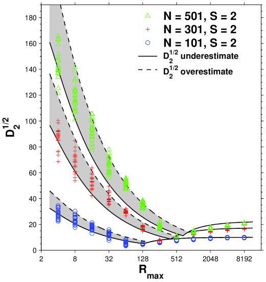
Figure 1: (Color online) Results for the standard deviation of fluctuations $D_{2}^{1/2}$ in the Minority Game. Numerical results correspond to 20 different runs at each $N$ and $R_{\rm max}$. The theoretical curves are generated using the analytic expressions in the text. The shaded area bounded by the upper and lower curves shows our theoretical prediction of the numerical spread for a given $N$. In line with the original numerical results of Ref. savit , we have chosen successive $R_{\rm max}$ tick-values to increase by a factor of 4.

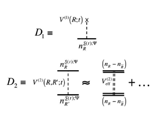
Figure 2: Diagrammatic equivalent (schematic) of some simple $p$th order moments $D_{P}$ of the multi-agent output variable $D(t)$. Top: $p=1$ is the mean $D_{1}$. Bottom: $p=2$ is the variance $D_{2}$. Also shown is an approximate expansion for $D_{2}$ as represented by Eq. (8). Higher-order terms, which are neglected in Eq. (8), would correspond to residual correlations between distinct Crowd-Anticrowd quasiparticles.

References

- (1) J.L. Casti, Would-be Worlds (Wiley, New York, 1997). See also http://sbs-xnet.sbs.ox.ac.uk/complexity/complexitysplash2003.asp
- (2) See http://www.unifr.ch/econophysics/minority
- (3) A. Soulier and T. Halpin-Healy, Phys. Rev. Lett. 90, 258103 (2003); A. Bru, S. Albertos, J.A. Lopez Garcia-Asenjo, and I. Bru, Phys. Rev. Lett. 92, 238101 (2004); B. Huberman and R. Lukose, Science 277, 535 (1997); B. Arthur, Amer. Econ. Rev. 84, 406 (1994); J.M. Epstein, Proc. Natl. Acad. Sci. 99, 7243 (2002). See also the works of D. Wolpert and K. Tumer at http://ic.arc.nasa.gov
- (4) N.F. Johnson and P.M. Hui, cond-mat/0306516; N.F. Johnson, P. Jefferies, P.M. Hui, Financial Market Complexity (Oxford University Press, 2003).
- (5) D. Challet and Y.C. Zhang, Physica A 246, 407 (1997); D. Challet, M. Marsili and R. Zecchina, Phys. Rev. Lett. 82, 2203 (1999); J.A.F. Heimel, A.C.C. Coolen and D. Sherrington, Phys. Rev. E 65, 016126 (2001); A. Cavagna, J.P. Garrahan, I. Giardina and D. Sherrington, Phys. Rev. Lett. 83, 4429 (1999).
- (6) R. Savit, R. Manuca and R. Riolo, Phys. Rev. Lett. 82, 2203 (1999).
- (7) N.F. Johnson, P.M. Hui, R. Jonson and T.S. Lo, Phys. Rev. Lett. 82, 3360 (1999); S. Hod and E. Nakar, Phys. Rev. Lett. 88, 238702 (2002); E. Burgos, H. Ceva, and R.P.J. Perazzo, Phys. Rev. Lett. 91, 189801 (2003); R. D’hulst and G.J. Rodgers, Physica A 270, 514 (1999). These works focus on probabilistic strategies.
- (8) N.F. Johnson, M. Hart and P.M. Hui, Physica A 269, 1 (1999); M. Hart, P. Jefferies, N.F. Johnson and P.M. Hui, Physica A 298, 537 (2001); S.C. Choe, P.M. Hui and N.F. Johnson, Phys. Rev. E 70, 055101(R) (2004); M. Hart, P. Jefferies, N.F. Johnson and P.M. Hui, Phys. Rev. E 63, 017102 (2001).
- (9) P. Jefferies, M.L. Hart and N.F. Johnson, Phys. Rev. E 65, 016105 (2002).
- (10) F.K. Chow and H.F. Chau, Physica A 337, 288 (2004); Physica A 319, 601 (2003); K.H. Ho, W.C. Man, F.K. Chow and H.F. Chau, cond-mat/0411554.
- (11) G.D. Mahan, Many-Particle Physics (Plenum Publishing, New York, 2000) 3rd Edition.
- (12) D. Challet and N.F. Johnson, Phys. Rev. Lett. 89, 028701 (2002).
- (13) We interchange the order of the and -averaging over the product of the ’s. Numerical simulations suggest this is valid for the systems of interest.
- (14) T.S. Lo, K.P Chan, P.M. Hui, N.F. Johnson, cond-mat/0409140.